Imputation of Missing PM_2.5 Observations in a Network of Air Quality Monitoring Stations by a New kNN Method

Abstract

Statistical analyses often require unbiased and reliable data completion. In this work, we imputed missing fine particulate matter (PM_2.5) observations from eight years (2012–2019) of records in 59 air quality monitoring (AQM) stations in Israel, using no auxiliary data but the available PM_2.5 observations. This was achieved by a new k-Nearest Neighbors multivariate imputation method (wkNNr) that uses the correlations between the AQM stations’ data to weigh the distance between the observations. The model was evaluated against an iterative imputation with an Ensemble of Extremely randomized decision Trees (iiET) on artificially and randomly removed data intervals of various lengths: very short (0.5–3 h, corresponding to 1–6 missing values), short (6–24 h), medium-length (36–72 h), long (10–30 d), and very long (30 d–2 y). The new wkNNr model outperformed the iiET in imputing very short missing-data intervals when the adjacent lagging and leading observations were added as model inputs. For longer missing-data intervals, despite its simplicity and the smaller number of hyperparameters required for tuning, the new model showed an almost comparable performance to the iiET. A parallel Python implementation of the new kNN-based multivariate imputation method is available on github.

1. Introduction

Due to the irrefutable evidence of causal associations between exposure to ambient pollutants, especially fine particulate matter (PM_2.5), and adverse health outcomes [1,2,3,4,5,6,7], air quality monitoring (AQM) networks have been established in the past decades to track pollutant levels. The higher the spatiotemporal measurement coverage, the higher the ability of regulatory agencies to enforce environmental standards and to derive reliable risk estimates for assessing the true cost of air pollution to society. However, oftentimes, monitoring data suffer from periods of missing records as a result of device failure, calibration procedures, maintenance, limited communication, or other technical difficulties. Imputation of missing records may be a prerequisite for advanced statistical analyses that require a complete dataset, like matrix factorization-based source apportionment methods.

In general, the imputation of AQM stations’ data can be carried out using either univariate or multivariate methods. In univariate imputation, each PM_2.5 time-series that has been measured by any AQM station is independently imputed. Univariate imputation can be performed by different methods, such as linear-, spline- or Nearest Neighbor (NN) interpolations [8,9]; spectral methods, e.g., Discrete Fourier Transform (DFT) [10,11]; or variations of Recurrent Neural Networks (RNN), which can capture long-term temporal dependencies [12,13]. In multivariate imputation, the AQM network is viewed as a multivariate dataset, where at each observation time-point there are several PM_2.5 measurements gathered simultaneously at different AQM stations. While univariate imputation relies only on the non-missing data from the imputed series itself (i.e., utilizing temporal relationships), multivariate methods can leverage from relationships among different co-measured time-series (i.e., accounting also for spatial relationships) [14,15,16]. Hence, multivariate imputation methods have been found to outperform univariate methods when imputing long periods of missing data [17].

The k-Nearest Neighbors (kNN) algorithm [18] has been widely used for multivariate imputations and was found to perform well when applied to environmental datasets [19,20]. Traditionally, the average of the non-missing values from the k most similar observations is used to fill in the missing value, where the similarity between any two observations is defined as the Euclidean distance between them. Different modifications to this simple kNN method demonstrated improved performance. For example, Troyanskaya et al. [21] took a weighted average of the values from the k most similar genes, based on an inverse Euclidean distance, to impute a gene-array; Pan and Li [22] utilized a linear regression model to account for spatial relationships between pairs of nodes in a network of wireless sensors; Feng et al. [23] discarded surrounding gauging stations below a certain correlation threshold when imputing monthly rainfall data, and Brás and Menezes [24] and Zhang [25] suggested an iterative process for fine adjustment of the imputed values. All these studies have shown the advantages of using multivariate kNN models over other methods (e.g., singular-value decomposition (SVD); [21]), yet none was applied to real-world air pollution data. In particular, PM_2.5 is a complex mixture of airborne particles whose dispersion is governed in a highly non-linear manner by meteorological conditions, physicochemical processes, and removal mechanisms [26,27,28,29]. Hence, to obtain satisfying results, most PM_2.5 imputation studies, to date, used auxiliary data, such as co-measured concentrations of other pollutants, meteorological parameters [17,30,31,32,33], or the output of atmospheric chemistry and transport models [16].

This work examines a new multivariate kNN imputation method (wkNNr), applied on a large and naturally incomplete PM_2.5 dataset that is comprised of eight years (2012–2019) of half-hourly observations from 59 AQM stations spread across Israel. The work extends beyond past studies in the following ways: (i) the new method uses the correlations between the AQM stations’ records to weigh the distance between observations, (ii) lagging and leading observations are accounted for as additional model inputs that can supply information on short-term temporal associations, and (iii) the imputation is based only on the non-missing PM_2.5 records in the dataset, thus enabling the use of other auxiliary data in advanced analyses without fearing collinearity. We compared the new model results to those obtained by applying an iterative imputation scheme, which has been shown to outperform many other imputation algorithms and was therefore chosen to serve as a benchmark. We evaluated the performance of the new method on randomly removed time-intervals of various lengths, using three performance metrics: normalized root mean squared error (NRMSE), coefficient of determination (R²), and normalized mean absolute error (NMAE). The imputation models’ performance was evaluated for each AQM station and different lengths of artificially removed data intervals, and the influence of seasonality was also examined. A parallel Python implementation of the new kNN-based multivariate imputation method is available on github.

2. Materials and Methods

2.1. Study Area and Data

PM_2.5 observations were obtained from the Technion Center of Excellence in Exposure Science and Environmental Health (TCEEH) Air Pollution Monitoring Database (TAPMD). The TAPMD holds all the air quality monitoring (AQM) records observed in Israel since 1995, collected by the Ministry of Environmental Protection (MoEP) and by other agencies, using EPA-approved instruments. The data have passed a routine quality assurance procedure [29]. The number of reporting AQM stations increased around 2011 due to the phase-in of the Israel Clean Air Act. Thus, we limited the study period to the years 2012–2019, resulting in a dataset of, at most, 140,256 half-hourly observations in each of the AQM stations whose data were used.

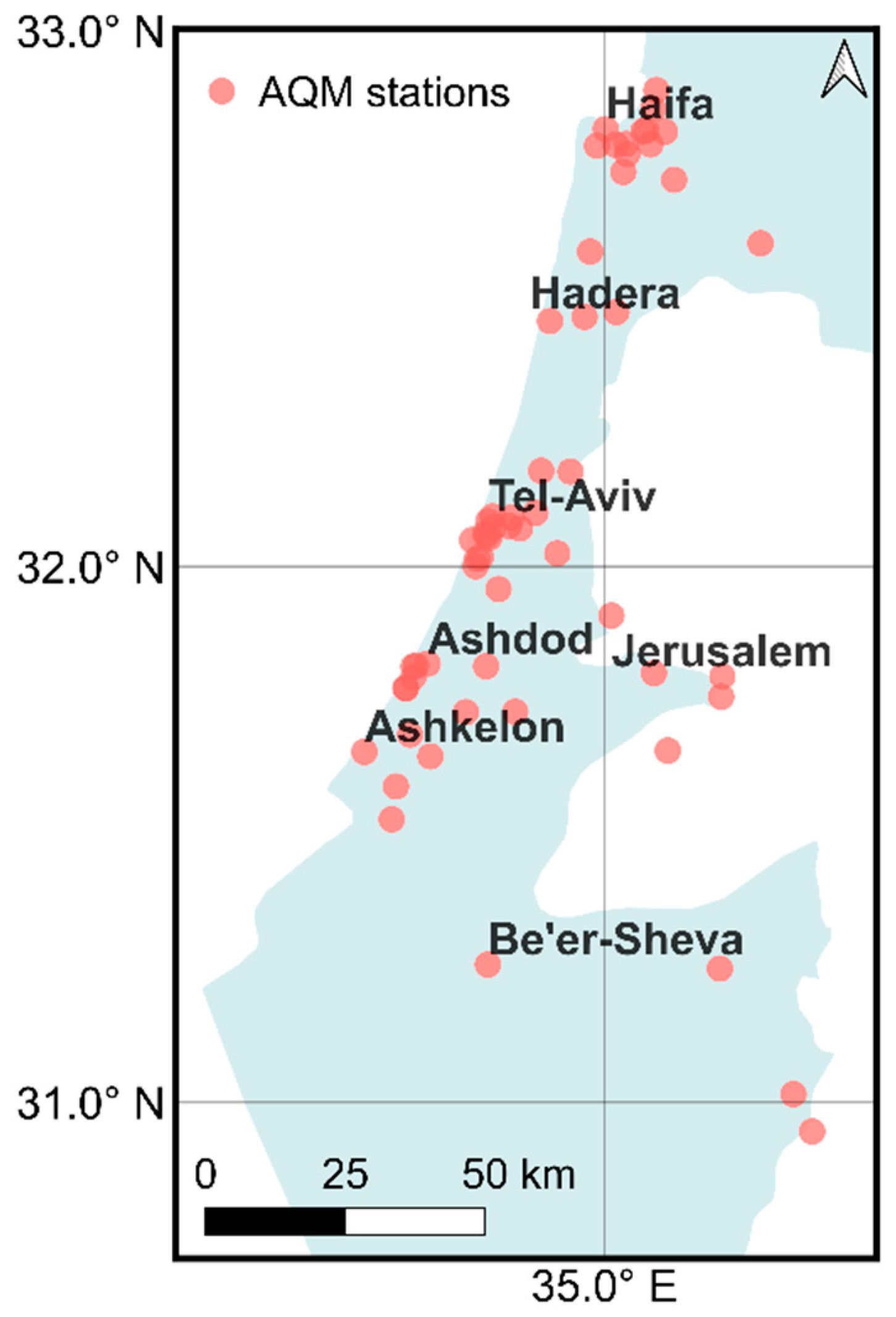
We used all the 59 AQM stations (Figure 1) that operated during the study period and monitored fine airborne particles (PM_2.5). Most PM_2.5 AQM stations in Israel are situated around five densely populated metropolitan areas (Figure 1): (i) Haifa, in the northern coastal plain, (ii) Tel-Aviv (Gush Dan), in the central coastal plain, (iii) Jerusalem, in the Judah Mountains, (iv) Ashdod, in the southern coastal plain, and (v) Ashkelon, which is also located in the southern coastal plain. The 2012–2019 PM_2.5 annual means and standard deviations (SD) in these areas were 17.9 (1.4) μg/m³, 22 (1.5) μg/m³, 19.8 (2.5) μg/m³, 20.7 (1.5) μg/m³, and 19.1 (1.1) μg/m³, respectively. These levels exceed the World Health Organization (WHO) recommended PM_2.5 annual mean (5 μg/m³) as well as the annual US National Air Quality Standards (NAQS) for PM_2.5 (12 μg/m³). The major local anthropogenic PM_2.5 sources in Israel are transportation and industrial plants. However, a substantial fraction of the total observed PM_2.5 levels results from transboundary transport that is carried to Israel during certain synoptic conditions. For example, mineral dust is carried to the region from the Sahara Desert and the Arabian Peninsula during the winter and the transition seasons, while secondary/ aged particles are transported to Israel from eastern and southern Europe mainly in the summer. Clearly, the particles that reach Israel as part of this long-range transboundary transport have different physicochemical properties (size distribution, composition, etc.), and the phenomena are characterized by distinct intensity (concentrations) and length (duration) [34,35,36,37,38].

2.2. Missing-Data Characteristics

Twenty-three out of the 59 AQM stations in the dataset were characterized by poor data coverage, each with accumulated missing observations of >4 years during the study period (i.e., >50% missing observations). Thus, although missing observations were imputed in all the 59 AQM stations, we did not use the latter 23 AQM stations for model evaluation, due to the inevitable higher uncertainty in their imputed values.

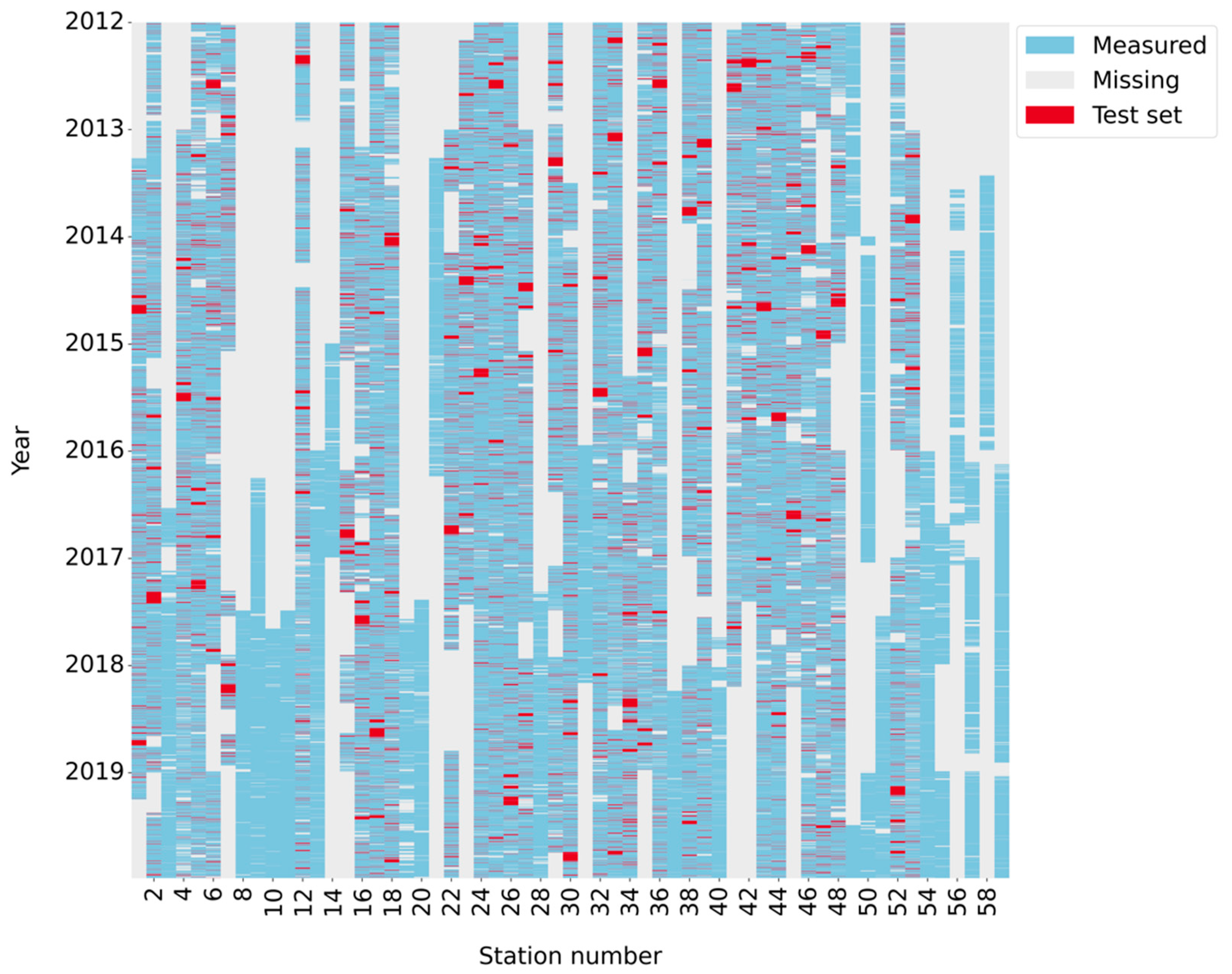
On average, the percentage of missing PM_2.5 observations (out of the total possible 140,256 observations) in the 36 AQM stations with <4 years of accumulated missing observations was 20.4%, with a median and a SD of 22% and 12.9%, respectively.

Table 1. Frequency distribution of the actual missing-data intervals in the dataset, grouped into six length (L) categories. Statistics is reported only for the 36 AQM stations with accumulated missing observations ≤4 years (marked in bold in Table S1 in the Supplementary Materials). The AQM observations are reported every 0.5 h.

Length of Missing Data Interval (L)	Length Category	Fraction of Missing Data Intervals out of the Total Number of Missing Intervals (%)	Fraction of Missing Observations out of the Total Number of Missing Observations (%)
L ≤ 3 h	very short	92.88	7.44
3 h < L ≤ 24 h	short	5.32	4.33
24 h < L ≤ 7 d	medium length	1.45	9.01
7 d < L ≤ 30 d	long	0.22	7.20
30 d < L ≤ 2 y	very long	0.12	53.91
2 y < L ≤ 4 y	extremely long	0.01	18.11

presents the distribution of lengths of the missing-data intervals in these 36 AQM stations. About 93% of the missing PM_2.5 intervals were very short (≤3 h), however, their total missing time points accounted only for about 7% of the overall missing observations. Figure 2 depicts the temporal coverage of these 36 AQM stations’ datasets, with missing values marked in grey. The mechanism responsible for the missing observations has a profound influence on the characteristics that are presented in Table 1 and Figure 2, as well as on the imputation performance. For standard air quality monitoring data, it is common to assume a “missing at random” (MAR) mechanism [17,39,40], with the probability of an observation to be missing independent of the missing value itself, although it might be influenced by an external cause [41].

2.3. Workflow

The research workflow included the following steps:

(i)

Setting aside a test set for the imputation models’ performance evaluation. For each AQM station, this set included N randomly sampled chunks of observations of length L, denoted hereafter “time-windows” (N $\times$ L: 720 $\times$ 0.5 h, 360 $\times$ 1 h, 180 $\times$ 2 h, 120 $\times$ 3 h, 120 $\times$ 6 h, 30 $\times$ 24 h (1 d), 20 $\times$ 36 h, 10 $\times$ 72 h, 3 $\times$ 240 h (10 d), and 1 $\times$ 720 h (30 d, i.e., 1 m)), that were artificially designated as missing (marked in red in Figure 2). The artificially removed data intervals were categorized into four categories: very short (0.5 h, 1 h, 2 h, 3 h), short (6 h, 24 h), medium-length (36 h, 72 h), and long (10 d, 30 d). Overall, in each of the 36 AQM stations with accumulated missing observations ≤4 years (marked in bold in Table S1 in the Supplementary Materials), 11,520 time points (half hours) served as the test set, corresponding on average to 11% (9–17%) of the non-missing observations.

(ii)

Tuning the models’ hyperparameters using a cross-validation (CV) procedure with repeated random sub-sampling of the training set (marked in blue in Figure 2). In each iteration, a sub-sample of the training set was designated as missing and served as a validation set against which the model performance was examined for different hyperparameters. The tuning of the hyperparameters was conducted separately for the very short, short, medium-length, and long time-window categories of the artificial missing data. Each of these category-based sub-samples accounted for 12% (9–20%) of the training set.

Figure 2. Temporal coverage of PM_2.5 observations at the 59 AQM stations in the years 2012–2019. Grey—missing observations, blue and red—non-missing observations. Blue—the training set, red—the test set used for model evaluation, comprised of randomly selected artificially missing time-windows of different lengths (0.5 h, 1 h, 2 h, 3 h, 6 h, 24 h, 36 h, 72 h, 10 d, and 30 d). Station names are specified in Table S1 in the Supplementary Materials. The test set (red) was extracted only from the 36 AQM stations with accumulated missing data of ≤4 years.

Figure 2. Temporal coverage of PM_2.5 observations at the 59 AQM stations in the years 2012–2019. Grey—missing observations, blue and red—non-missing observations. Blue—the training set, red—the test set used for model evaluation, comprised of randomly selected artificially missing time-windows of different lengths (0.5 h, 1 h, 2 h, 3 h, 6 h, 24 h, 36 h, 72 h, 10 d, and 30 d). Station names are specified in Table S1 in the Supplementary Materials. The test set (red) was extracted only from the 36 AQM stations with accumulated missing data of ≤4 years.

(iii)

Building the imputation models using the training set and the models’ optimal hyperparameters.

(iv)

Evaluation of the performance of the imputation models on the test sets for each of the 36 AQM stations and for the four categories of missing-data interval length (very short, short, medium-length, and long). The following metrics were used for evaluating the models’ performance (see Table S2 in the Supplementary Materials): normalized root mean squared error (NRMSE), coefficient of determination (R²), and normalized mean absolute error (NMAE). The normalization of the metrics was required to enable comparison across missing-data interval lengths, seasons, and geographic regions (i.e., different AQM stations). We compared the imputation performance of the different models using the non-parametric Kruskal-Wallis one-way analysis of variance, followed by the Conover-Iman post-hoc test [42]. Furthermore, we examined how the model performance varied among seasons by means of Taylor diagrams [43].

(v)

Finally, a test-case of a very long (2 years) missing-data interval was examined, to inspect the ability of the models to handle large missing-data intervals. For this, we randomly removed two years of records (i.e., a sequence of 35,040 time points) from 25 AQM stations (one at a time) that had less than two years of accumulated missing observations. For each of these AQM stations, we ran the imputation models with the optimal hyperparameters found for the long (7 d< L ≤ 30 d) missing-data time-window (Tables S3 and S4 in the Supplementary Materials).

2.4. Model Description

2.4.1. Multivariate Weighted-kNN Imputation Using Correlations (wkNNr)

In this work the traditional kNN multivariate imputation has been modified as follows: (i) we modified the Euclidean distance function such that differences between observations in AQM stations that showed high correlations with the imputed AQM station obtained higher weights, and (ii) we used the inverse of this distance function for calculating the weighted average of the k-nearest observations. In general, the method follows these steps: for a matrix $X$ of $N$ PM_2.5 observations in $M$ AQM stations ($X_{\left[N\times M\right]}$), let $x_{ij}$ denote the $i$th observation in the $j$th AQM station, and let $O\left(x_{ij}\right)$ denote whether the value of $x_{ij}$ is missing:

$$O\left(x_{ij}\right)=\left\{\begin{array}{cc}0\hfill & \hfill \mathrm{if} x_{ij} \mathrm{is} \mathrm{missing}\hfill \\ 1\hfill & \hfill \mathrm{otherwise}\hfill \end{array}\right.$$

(1)

Let $Common\left(i,n,m\right)=O\left(x_{im}\right)·O\left(x_{nm}\right)$ such that $Common\left(i,n,m\right)=1$ if rows $i$ and $n$ both have non-missing observations in column $m$ and $Common\left(i,n,m\right)=0$ otherwise. In addition, let

$$Common\left(i,n\right)={{\displaystyle \sum }}_{m=1}^{M}Common\left(i,n,m\right)$$

(2)

such that $Common\left(i,n\right)$ is the number of columns with non-missing observations in both rows $i$ and $n$. For each missing value $x_{ij}$ to be imputed, we define a correlation-weighted distance function between the observations in the $i$th and the $n$th rows (Equation (3)),

$$Dis{t}_{ij}\left(n\right)=\sqrt{\frac{{{\displaystyle \sum }}_{m=1}^M Common\left(i,n,m\right) · {(x_{im}-x_{nm})}^2 · r_{mj}^2}{Common\left(i,n\right)}}$$

(3)

where $r_{mj}$, the correlation between columns m and j, acts as a weighing coefficient of the distance function. Namely, the distance function takes into account the correlation between the AQM stations, such that measurement differences in AQM stations that are correlated with the imputed AQM station (marked by j in Equation (3)) contribute more to the distance metric while measurement differences in uncorrelated AQM stations are discounted. This gives preference to rows with smaller distances in AQM stations that are highly correlated with the currently imputed one. For imputing the missing value $x_{ij}$, we define a weight function:

$$W_{ij}\left(n\right)=\frac{Common{\left(i,n\right)}^q}{Dis{t}_{ij}\left(n\right)}$$

(4)

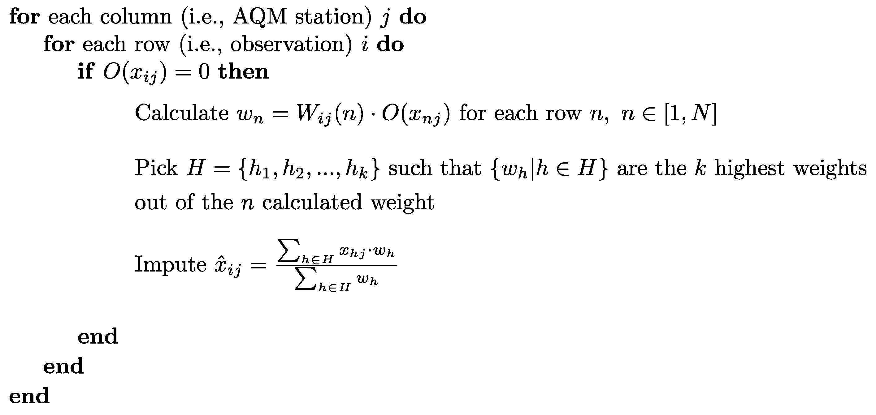
In Equation (4), $Common\left(i,n\right)$ is raised to a power of q to give preference to rows with fewer missing values, i.e., with a larger $Common\left(i,n\right)$, since the reliability of these rows is higher. A missing value in the $i$th row and the $j$th column is imputed by taking the weighted average of the non-missing values in the $j$th column from the k rows with the highest weights. The overall imputation procedure is described in the following pseudo-code (Figure 3).

We tuned the hyperparameters (k, q, type of correlation) using a grid search optimization, with the loss function being the average RMSE of 10 sub-samples randomly drawn from the training set during the CV procedure. The search space and the optimal hyperparameters are detailed in Table S3 in the Supplementary Materials.

2.4.2. Multivariate Iterative Imputation with Extra Trees (iiET)

As a benchmark imputation method, we applied a variation of the missForest iterative imputation algorithm [44], available in the IterativeImputer class of the scikit-learn Python library [45]. The missForest algorithm was found to outperform many other imputation methods [23,46,47,48]. However, while the original missForest algorithm iteratively trains a Random Forest (RF) estimator on the observed values [49], the iterative imputation method we applied trains a faster tree ensemble—the extremely randomized decision trees (Extra Trees, ET) estimator [50]. Specifically, whereas a decision tree in a RF splits each node by the best possible split among a random subset of features (i.e., AQM stations) selected at each node, the ET algorithm employs a faster feature selection via randomization. The ET algorithm first sets a random threshold value for each feature as a potential split, and then selects the feature with the best split among them. Additionally, the ET algorithm uses the whole learning sample to grow the trees [50] while the RF draws observations with replacement (bootstrapping). We designated the iterative imputation algorithm based on the extremely randomized decision trees, i.e., the benchmark model, iiET.

The iiET imputation follows these steps: the time-series of one AQM station is designated as the output (y) and the other AQM stations’ records are treated as input (X). An ET regression estimator is then fitted on (X, y) for all the known values in y. Next, the estimator predicts the missing values in y. These steps are performed on each of the AQM station’s time series, starting from the AQM station with the fewest missing values and progressing to AQM stations with more missing values. The procedure is repeated up to the preset maximum number of iterations (n), refining the estimation of the missing values in each iteration. Often, a small number of iterations is sufficient for convergence [51,52]. The following hyperparameters of the ET estimator (the kernel of the iiET model) were tuned: the number of trees in an ensemble (‘n_estimators’), the minimum number of samples in each leaf node (‘min_samples_leaf’), and the minimum number of samples required to split a node (‘min_samples_split’). For the tuning, we used a Bayesian optimization model with 40 iterations [53] and with the loss function being the average RMSE of 10 sub-samples. Subsequently, we tuned the number of iterations of the iiET model, n. The search-space and optimal hyperparameters are detailed in Table S4 in the Supplementary Materials.

2.5. Accounting for Adjacent Lagging and Leading Observations

To improve the performance of both imputation methods, we examined accounting also for the first and second lagging and leading observations, denoting these models by a “ll₁” or a “ll₂” suffix, respectively. For example, wkNNr_ll₁ is the wkNNr method when it accounts also for two additional time-series beyond the time-series that we wish to impute as input: one that leads and one that lags the imputed time-series by one timestep (half an hour). This results in operation on a dataset that is three times larger. Similarly, the wkNNr_ll₂ operates on a dataset that is five times larger since it accounts for two lagging and two leading time-series beyond the currently imputed time-series. We were able to account for the first and second lagging and leading observations in the wkNNr model (denoting these models wkNNr_ll₁ and wkNNr_ll₂, respectively). However, due to the very high computational demand (RAM) of the iiET model, using this model we could only account for the first lagging and leading observations (denoting the model iiET_ll₁). We evaluated the optimal number, T, of the lagging and leading observations to be used as model inputs by calculating the partial autocorrelation function for each AQM station’s time-series. The partial autocorrelation between observations at lag T is the correlation that results after removing the effect of all the shorter lags (<T) correlations. Applying this approach to our dataset, we found that most AQM stations had meaningful partial autocorrelations over only 1–2 lagging/leading half-hour time-points, suggesting that accounting for more distant observations is not expected to further improve the performance of the imputation models. We ran these enhanced models with the optimal hyperparameters obtained for the wkNNr and the iiET models (see Section 2.4 and Tables S3 and S4 in the Supplementary Materials).

3. Results

We report here the results of steps (iii)–(v) of the workflow (Section 2.3). The results of step (ii) (tuning of the models’ hyperparameters) are reported in Tables S3 and S4 in the Supplementary Materials. For simplicity, all the variations of the wkNNr and iiET methods (i.e., wkNNr and iiET with the lagging and leading observations added as inputs), are referred to as different models.

3.1. Model Performance for Different Missing-Data Time-Window Lengths

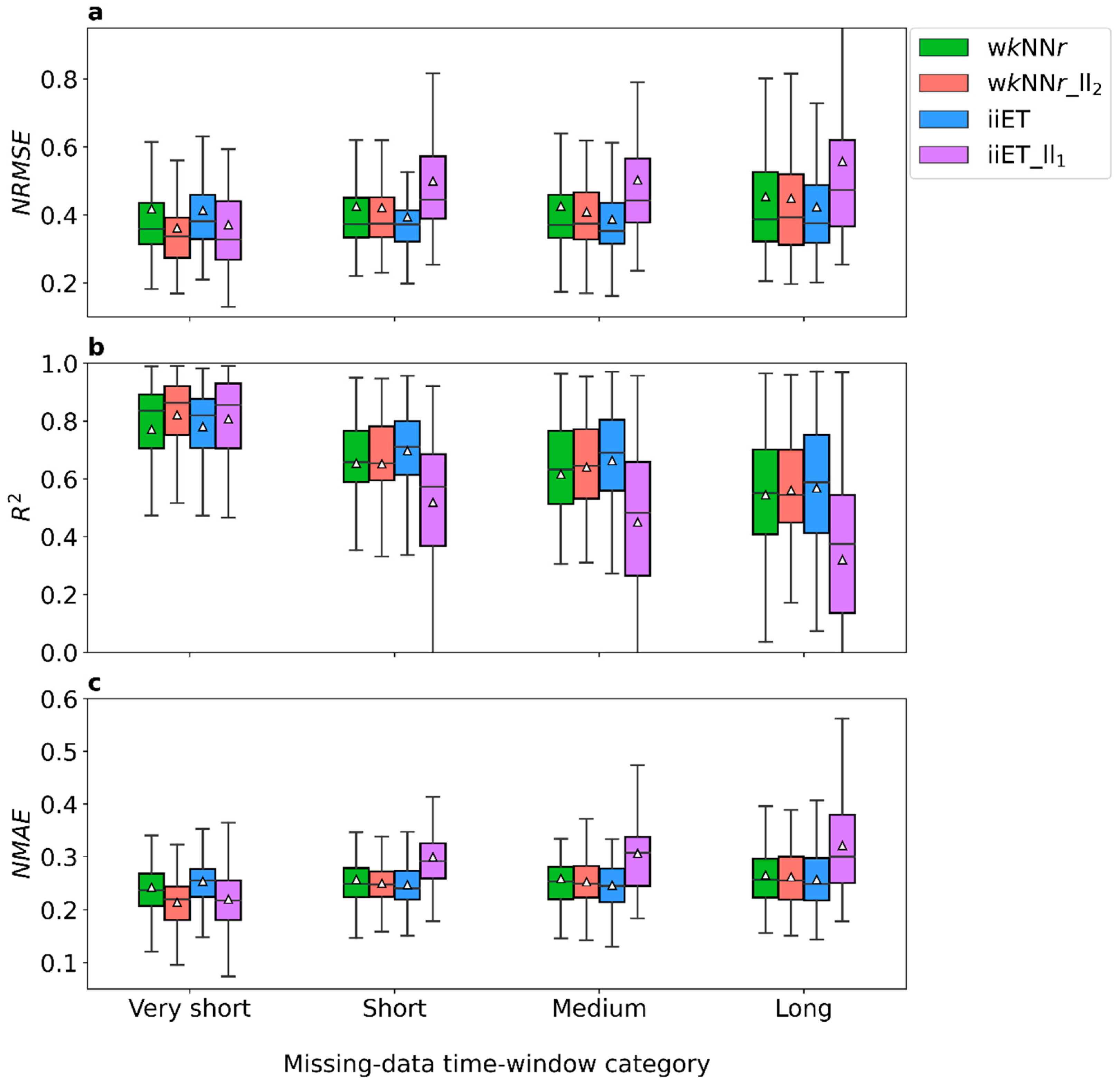
After the different imputation models were employed with the selected optimal hyperparameters, their performance was evaluated. We report here the models’ performance at each AQM station for the first four missing-data time-window length categories (Figure 4 and Table 2). Since the wkNNr_ll₂ model was found to perform slightly better than the wkNNr_ll₁ model, the latter is not reported hereinafter.

On average, for the very short (0.5–3 h) missing-data time-windows the wkNNr_ll₂ model showed significantly better (p < 0.05) performance than all the other models (Figure 4 and Table 2). It is noteworthy that while the performance of the iiET_ll₁ model was similar to that of the wkNNr_ll₂ for the very short missing-data time-windows (in terms of the NRMSE, R², and NMAE), the iiET_ll₁ model showed a significantly higher (p < 0.05) normalized mean bias (NMB, see Table S2; wkNNr_ll₂: 0.021 ± 0.03, iiET_ll₁: 0.062 ± 0.06). Moreover, while the iiET model showed the best performance for the longer missing-data time-window categories (Figure 4 and Table 2), the differences between the wkNNr_ll₂ and the iiET models in terms of all the performance measures were not significant (Table 2).

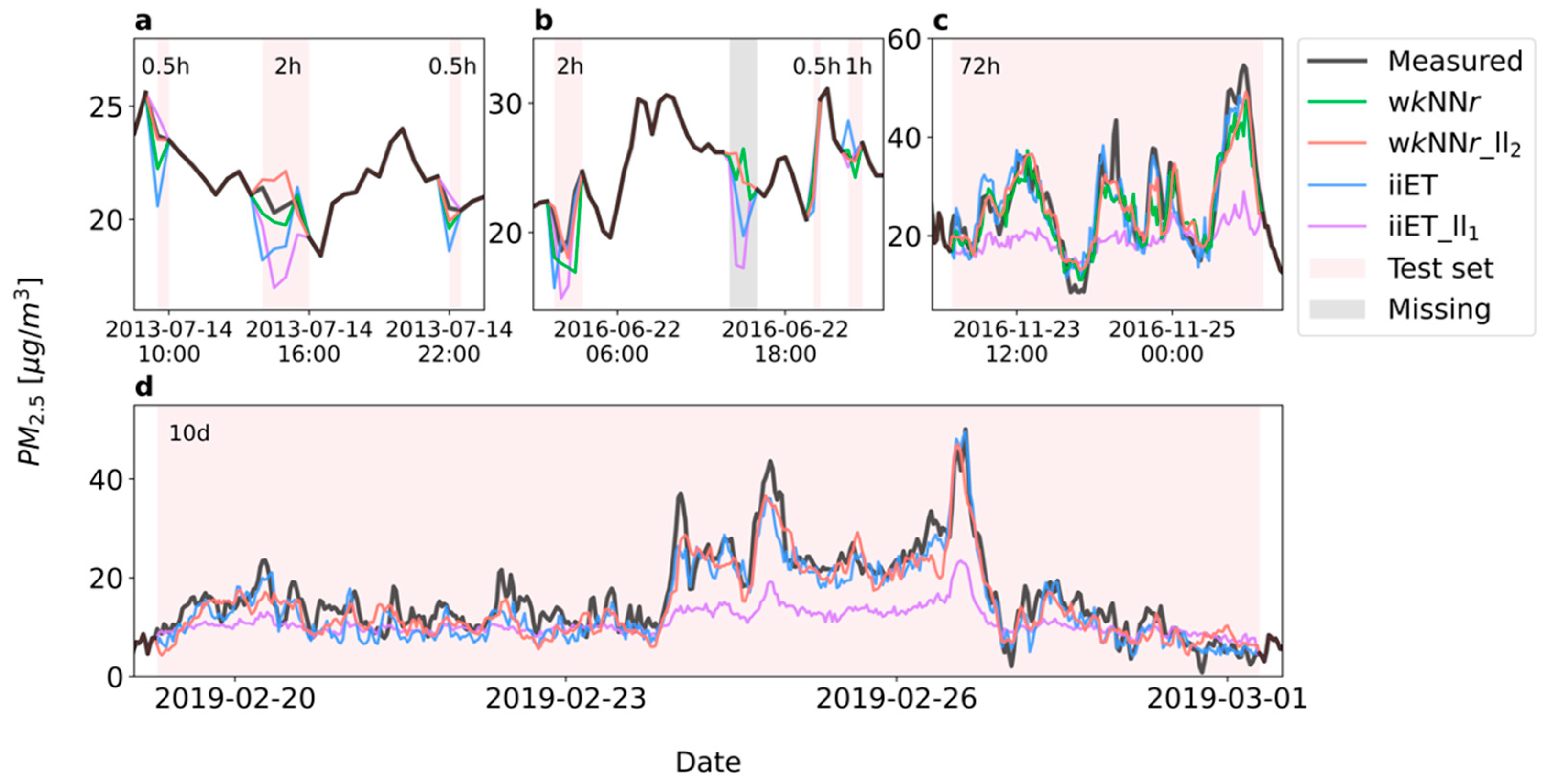
A few examples of missing-data time-series imputations are depicted in Figure 5. For very short missing-data time-windows, imputation by the wkNNr_ll₂ model generally provided better results than those obtained by all the other models (Figure 5a,b), in agreement with Figure 4. The performance deterioration of the iiET_ll₁ model is seen already in the imputation of the 2 h missing-data time-window (Figure 5a,b). For the imputation of longer missing-data time-windows (Figure 5c,d), the advantage of the iiET model over the wkNNr_ll₂ model is evident when rapid concentration changes occurred.

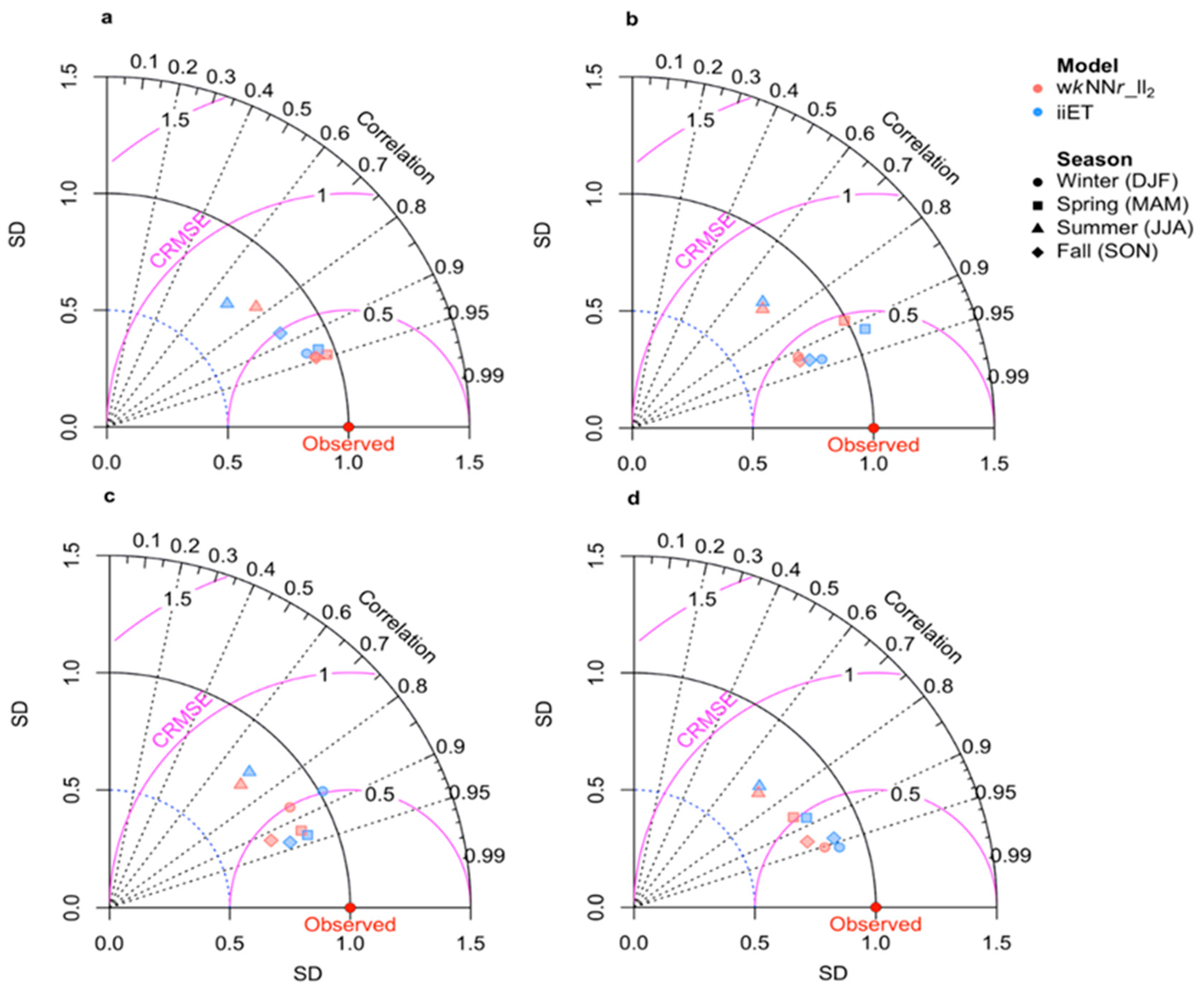
The Taylor diagrams (Figure 6) depict seasonal changes in the iiET and wkNNr_ll₂ models’ performance, revealing lower imputation performance for all the missing-data time-window categories during the summer (JJA) relative to the other seasons. This is evident by a higher normalized centered RMSE (CRMSE, see Table S2 in the Supplementary Materials) and a lower correlation between the measured and imputed PM_2.5 concentrations in the summer (see Discussion).

Figure 4. Model performance in terms of (a) NRMSE, (b) R², and (c) NMAE. Each boxplot contains all the imputation evaluation results in the 36 AQM stations (see Section 2.2), categorized according to the missing-data time-window length: very short (0.5–3 h), short (6–24 h), medium-length (36–72 h), and long (10–30 d), with N = 144, 72, 72, and 72, respectively. White triangles: mean values, black horizontal lines: median values, lower and upper box boundaries mark the 25th and 75th percentiles, respectively (i.e., the inter quartile range, IQR). The upper whisker represents the 75th percentile + 1.5 $\times$ IQR, and the lower whisker represents the 25th percentile − 1.5 $\times$ IQR. Outliers are not shown to avoid clutter.

Figure 4. Model performance in terms of (a) NRMSE, (b) R², and (c) NMAE. Each boxplot contains all the imputation evaluation results in the 36 AQM stations (see Section 2.2), categorized according to the missing-data time-window length: very short (0.5–3 h), short (6–24 h), medium-length (36–72 h), and long (10–30 d), with N = 144, 72, 72, and 72, respectively. White triangles: mean values, black horizontal lines: median values, lower and upper box boundaries mark the 25th and 75th percentiles, respectively (i.e., the inter quartile range, IQR). The upper whisker represents the 75th percentile + 1.5 $\times$ IQR, and the lower whisker represents the 25th percentile − 1.5 $\times$ IQR. Outliers are not shown to avoid clutter.

Table 2. Mean (standard deviation) of the performance measures for the different missing-data time-window categories.

Category	Model	NRMSE	R2	NMAE
Very short	wkNNr	0.42 (0.22)	0.77 (0.19)	0.24 (0.06)
	wkNNr_ll2	0.36 (0.16)	0.82 (0.13)	0.21 (0.05)
	iiET	0.41 (0.17)	0.78 (0.14)	0.25 (0.05)
	iiET_ll1	0.37 (0.21)	0.81 (0.16)	0.22 (0.07)
p value a		<0.001	0.004	<0.001
Significant differences b		1, 4, 5, 6	1, 4, 5, 6	1, 3, 4, 5, 6
Short	wkNNr	0.43 (0.17)	0.65 (0.18)	0.26 (0.06)
	wkNNr_ll2	0.42 (0.16)	0.65 (0.24)	0.25 (0.04)
	iiET	0.39 (0.13)	0.70 (0.15)	0.25 (0.04)
	iiET_ll1	0.50 (0.16)	0.52 (0.25)	0.30 (0.06)
p value a		<0.001	<0.001	<0.001
Significant differences b		2, 4, 5	2, 4, 5	2, 4, 5
Medium length	wkNNr	0.43 (0.20)	0.62 (0.21)	0.26 (0.07)
	wkNNr_ll2	0.41 (0.15)	0.64 (0.18)	0.25 (0.05)
	iiET	0.39 (0.15)	0.66 (0.21)	0.25 (0.06)
	iiET_ll1	0.50 (0.20)	0.45 (0.28)	0.31 (0.07)
p value a		<0.001	<0.001	<0.001
Significant differences b		2, 4, 5	2, 4, 5	2, 4, 5
Long	wkNNr	0.45 (0.21)	0.55 (0.22)	0.27 (0.07)
	wkNNr_ll2	0.45 (0.20)	0.56 (0.21)	0.26 (0.06)
	iiET	0.42 (0.17)	0.57 (0.23)	0.26 (0.06)
	iiET_ll1	0.56 (0.29)	0.32 (0.37)	0.32 (0.09)
p value a		<0.001	<0.001	<0.001
Significant differences b		2, 4, 5	2, 4, 5	2, 4, 5

^a p value of the non-parametric Kruskal-Wallis test, applied on each measure across the four models. ^b Pairs of models that show statistically significant differences (p value < 0.05): (1) wkNNr_ll₂—iiET, (2) wkNNr_ll₂—iiET_ll₁, (3) wkNNr—iiET, (4) wkNNr—iiET_ll₁, (5) iiET—iiET_ll₁, (6) wkNNr—wkNNr_ll₂.

Table 2. Mean (standard deviation) of the performance measures for the different missing-data time-window categories.

Category	Model	NRMSE	R2	NMAE
Very short	wkNNr	0.42 (0.22)	0.77 (0.19)	0.24 (0.06)
	wkNNr_ll2	0.36 (0.16)	0.82 (0.13)	0.21 (0.05)
	iiET	0.41 (0.17)	0.78 (0.14)	0.25 (0.05)
	iiET_ll1	0.37 (0.21)	0.81 (0.16)	0.22 (0.07)
p value a		<0.001	0.004	<0.001
Significant differences b		1, 4, 5, 6	1, 4, 5, 6	1, 3, 4, 5, 6
Short	wkNNr	0.43 (0.17)	0.65 (0.18)	0.26 (0.06)
	wkNNr_ll2	0.42 (0.16)	0.65 (0.24)	0.25 (0.04)
	iiET	0.39 (0.13)	0.70 (0.15)	0.25 (0.04)
	iiET_ll1	0.50 (0.16)	0.52 (0.25)	0.30 (0.06)
p value a		<0.001	<0.001	<0.001
Significant differences b		2, 4, 5	2, 4, 5	2, 4, 5
Medium length	wkNNr	0.43 (0.20)	0.62 (0.21)	0.26 (0.07)
	wkNNr_ll2	0.41 (0.15)	0.64 (0.18)	0.25 (0.05)
	iiET	0.39 (0.15)	0.66 (0.21)	0.25 (0.06)
	iiET_ll1	0.50 (0.20)	0.45 (0.28)	0.31 (0.07)
p value a		<0.001	<0.001	<0.001
Significant differences b		2, 4, 5	2, 4, 5	2, 4, 5
Long	wkNNr	0.45 (0.21)	0.55 (0.22)	0.27 (0.07)
	wkNNr_ll2	0.45 (0.20)	0.56 (0.21)	0.26 (0.06)
	iiET	0.42 (0.17)	0.57 (0.23)	0.26 (0.06)
	iiET_ll1	0.56 (0.29)	0.32 (0.37)	0.32 (0.09)
p value a		<0.001	<0.001	<0.001
Significant differences b		2, 4, 5	2, 4, 5	2, 4, 5

^a p value of the non-parametric Kruskal-Wallis test, applied on each measure across the four models. ^b Pairs of models that show statistically significant differences (p value < 0.05): (1) wkNNr_ll₂—iiET, (2) wkNNr_ll₂—iiET_ll₁, (3) wkNNr—iiET, (4) wkNNr—iiET_ll₁, (5) iiET—iiET_ll₁, (6) wkNNr—wkNNr_ll₂.

Figure 5. Measured PM_2.5 concentrations (black line) vs. imputed concentrations by the wkNNr (green line), wkNNr_ll₂ (red line), iiET (blue line), and iiET_ll₁ (purple line) models for different missing-data time-window lengths (red shade). (a,b) Very short missing-data time-windows in AQM station #2, (c) a medium-length missing-data time-window in AQM station #15, and (d) a long missing-data time-window in AQM station #26 (the wkNNr model results are not shown to avoid clutter).

Figure 5. Measured PM_2.5 concentrations (black line) vs. imputed concentrations by the wkNNr (green line), wkNNr_ll₂ (red line), iiET (blue line), and iiET_ll₁ (purple line) models for different missing-data time-window lengths (red shade). (a,b) Very short missing-data time-windows in AQM station #2, (c) a medium-length missing-data time-window in AQM station #15, and (d) a long missing-data time-window in AQM station #26 (the wkNNr model results are not shown to avoid clutter).

Figure 6. Taylor diagrams of the wkNNr_ll₂ and iiET imputation models (represented by distinct colors) in the different seasons (represented by symbols): winter (DJF), spring (MAM), summer (JJA), and fall (SON). The plots correspond to different missing-data time-windows length categories: (a) very short, (b) short, (c) medium-length, and (d) long. The centered root mean squared error (CRMSE) is normalized by the standard deviation (SD) of the observations (see Table S2 in the Supplementary Materials).

Figure 6. Taylor diagrams of the wkNNr_ll₂ and iiET imputation models (represented by distinct colors) in the different seasons (represented by symbols): winter (DJF), spring (MAM), summer (JJA), and fall (SON). The plots correspond to different missing-data time-windows length categories: (a) very short, (b) short, (c) medium-length, and (d) long. The centered root mean squared error (CRMSE) is normalized by the standard deviation (SD) of the observations (see Table S2 in the Supplementary Materials).

3.2. A Test-Case of a Very Long Missing-Data Time-Window

Since the largest fraction of missing observations out of the total accumulated missing data was in the very long (30 d < L ≤ 2 y; Table 1) missing data category, we examined the performance of the imputation models in filling in such extended missing-data gaps (see Workflow (v)). Both the wkNNr_ll₂ and the iiET imputation models performed reasonably well even under such extreme test conditions, with mean (SD) NRMSE, R², and NMAE of 0.55 (0.25), 0.64 (0.23), and 0.29 (0.06) for the iiET model, and 0.59 (0.26), 0.61 (0.18) and 0.3 (0.05) for the wkNNr_ll₂ model.

4. Discussion

This work presents a new multivariate kNN imputation model that weighs the distance between the observations according to the correlation of the imputed AQM station’s time-series with all the other AQM stations’ time-series. To the best of our knowledge, this is the first study that applied such a model on a large dataset of PM_2.5 concentrations, achieving good accuracy without using any external data (e.g., meteorology, other air pollutants concentrations, land use) other than the available PM_2.5 concentrations in the dataset. The latter represents a considerable advantage due to the fewer input data required, and as it frees the auxiliary data for use as covariates in further analyses without fearing to introduce hidden relationships (e.g., collinearity) that can impair the results of the advanced analyses.

Since autocorrelations always exist in time-series of environmental observations, we hypothesized that accounting for the lagging and leading records around the imputed value could improve the models’ performance. Indeed, accounting for the first and second lagging and leading values as model inputs (wkNNr_ll₂) significantly improved the imputation of the very short missing-data time-windows by the wkNNr model. The result agrees with the studies of Junninen et al. [17] and Ottosen and Kumar [9], who showed the advantage of univariate interpolation methods for short missing-data gaps. The iiET_ll₁ model on the other hand showed poorer performance than the iiET model for all the time-window categories. The reason for this counterintuitive result is unclear and requires an in-depth examination that is beyond the scope of this work.

The wkNNr_ll₂ model showed the best imputation performance for very short missing-data time-windows (0.5–3 h) while the iiET model was superior in the imputation of longer missing-data time-windows (Figure 4 and Table 2). The superiority of the iiET model, a variation of the missForest algorithm, was expected due to its ability to learn complex relationships among the AQM stations’ data and to generalize them to unseen data. In addition, it uses an iterative process that enables fine-tuning of the final estimation. By contrast, the wkNNr and wkNNr_ll₂ models are inherently limited to estimating missing values based only on non-missing values in the imputed time-series, and they rely only on one correlation matrix. A possible way to improve the performance of the wkNNr model could be to account for several correlation matrices rather than just one, each accounting for a shorter time-period (e.g., one year instead of eight years). This might enable the imputation model to better respond to changes in the relationships between the AQM stations over time. Moreover, choosing the model inputs such that only AQM stations that are highly correlated with the AQM station that is being imputed are used could be advantageous. In this work, a zero-correlation threshold was set as a threshold for selecting the AQM stations that contribute to the distance calculation (Equation (3)). However, the option to apply other thresholds is implemented in the wkNNr code that has been reposited on github.

We found that the accuracy of the imputation varied between seasons (Figure 6), showing lower performance in the summer. This is likely related to the fact that PM_2.5 concentrations in the study area are considerably influenced by characteristic seasonal climatology [38], in particular, transboundary transport of PM of distinct nature by seasonally varying synoptic patterns [35]. In the East Mediterranean, mineral dust is transported from the north African Sahara and the Arabian deserts during all seasons but the summer, with the meteorological conditions characterized by an irregular succession of high-pressure systems, Red Sea troughs (a northward extension of the Sudan monsoon low), and eastern Mediterranean cyclones [34,37]. Such conditions generate high average Pearson correlations between AQM stations’ observations in the study area (0.6, 0.69, and 0.73 in the fall, winter, and spring, respectively), which enabled the models to impute relatively accurately missing observations in all the AQM stations. In contrast, the summer months in the East Mediterranean are characterized by stable and rather persistent atmospheric conditions but by varying anthropogenic emissions due to variations in electricity demands for air conditioning during the day and across regions, and due to summer vacation effects on traffic-related air pollution (TRAP). This variation generates considerable local variability across the AQM stations, and results in a lower average correlation between the AQM stations in the summer (r = 0.36). The latter hinders the ability of the imputation models to learn from the other AQM stations, resulting in lower imputation performance in the summer. Nevertheless, applying a moving-average smoothing of the time-series of both the measured and the imputed PM_2.5 revealed that even when a narrow moving average window (2 h) has been applied, the correlation between the observed and imputed smoothed time-series increased substantially for all the missing-data time-window categories. For example, for the long missing-data time-window category the correlation between the measured and the iiET imputed PM_2.5 concentrations increased in the summer from 0.7 (Figure 6d) to 0.81 after we applied a 2 h moving-average smoothing of the two time-series (not shown). These results demonstrate that if the performance of smoothed time-series is considered, the imputation models perform well even in the summer.

In general, an imputation scheme that uses only the non-missing PM_2.5 observations is expected to work well in situations where correlations between stations exist. Correlations could result from common emission sources or common climatology that may characterize relatively small regions, like our study area (Figure 1). Yet, correlations can also exist between distant AQM stations due to similar anthropogenic behavior (e.g., traffic patterns). Calculating the correlation matrix between all stations might be a good place to start when examining the applicability of the suggested imputation framework.

Furthermore, we note that the ability of imputation methods to fill in accurately missing AQM data highly depends on whether observed changes (e.g., long-term trends) were captured in the records of other AQM stations, i.e., whether these changes were local, e.g., the launching/ shutdown of a local industrial, quarrying, mining, or construction activity/ operation, or spatially global, e.g. a large-scale lasting trend. Hence, the imputation of long missing-data gaps in isolated AQM stations might be highly uncertain.

5. Conclusions

This work explored the use of a new method (wkNNr) for a reliable imputation of missing PM_2.5 observations in AQM records. To develop and evaluate the method we used eight years of data (2012–2019) from 59 AQM stations in Israel. Despite the mathematical simplicity of the wkNNr model, its comparable performance with the benchmark imputation model (iiET), and the significant (p < 0.05) improvement (R² = 0.82 compared with R² = 0.77) seen in the very-short missing-data time-windows when accounting for the lagging and leading observations as inputs (wkNNr_ll₂), attest for its robustness and strength. The wkNNr_ll₂ model carries both the advantage of univariate interpolation methods for short missing-data time gaps, and of multivariate methods for imputation of long missing-data gaps. With its small number of hyperparameters that require tuning (see Tables S3 and S4), preferring the wkNNr_ll₂ over the iiET would be a reasonable choice when time-resources are limited, and for datasets with mostly small missing gaps, which is common in environmental datasets (Table 1). Moreover, Table 2 reveals that in our dataset, the performance of the wkNNr_ll₂ model in the imputation of >3 h missing-data intervals was lagging only slightly and not significantly (p > 0.05) behind the performance of the iiET model. Alternatively, a hybrid model might be utilized, combining imputed values by the wkNNr_ll₂ in the very short missing-data gaps ($\le$3 h, corresponding to 1–6 missing values) with imputed values by the iiET in the longer missing-data gaps (>3 h missing values).

The imputation scheme developed in this study uses only the non-missing PM_2.5 observations, and as such. has a huge advantage if the imputed dataset should be used for further advanced analyses, e.g., unsupervised factorization methods for source apportionment. Namely, using only the PM_2.5 observations frees commonly used auxiliary data, such as meteorological records, concentrations of co-measured pollutants, etc., to be used as covariates in the advanced analyses without fearing that they had contaminated the dataset, e.g., inserted hidden relationships that can affect the source factors found.

The change in the model performance in the summer relative to the other seasons emphasizes the importance of climatology on PM_2.5 concentrations in the East Mediterranean. Hence, accounting for the season when calculating the correlation matrix can lead to an overall better performance of the wkNNr family of models. The unimputed dataset used in this work and the wkNNr models presented in this work are available at https://github.com/TCEEH/wkNNrImputation (accessed on 27 October 2022).

References

- Bräuner, E.V.; Forchhammer, L.; Møller, P.; Simonsen, J.; Glasius, M.; Wåhlin, P.; Raaschou-nielsen, O.; Loft, S. Exposure to ultrafine particles from ambient air and oxidative stress–induced DNA damage. Environ. Health Perspect. 2007, 115, 1177–1182. [Google Scholar] [CrossRef]
- Grahame, T.J.; Klemm, R.; Schlesinger, R.B. Public health and components of particulate matter: The changing assessment of black carbon. J. Air Waste Manag. Assoc. 2014, 64, 620–660. [Google Scholar] [CrossRef] [PubMed]
- Janssen, N.A.H.; Hoek, G.; Simic-Lawson, M.; Fischer, P.; van Bree, L.; Brink, H.; Keuken, M.; Atkinson, R.W.; Anderson, R.; Brunekreef, B.; et al. Black carbon as an additional indicator of the adverse health effects of airborne particles compared with PM10 and PM2.5. Environ. Health Perspect. 2011, 119, 1691–1699. [Google Scholar] [CrossRef] [Green Version]
- Krall, J.R.; Strickland, M.J. Recent approaches to estimate associations between source-specific air pollution and health. Curr. Environ. Health Rep. 2017, 4, 68–78. [Google Scholar] [CrossRef]
- de Prado Bert, P.; Mercader, E.M.H.; Pujol, J.; Sunyer, J.; Mortamais, M. The effects of air pollution on the brain: A review of studies interfacing environmental epidemiology and neuroimaging. Curr. Environ. Health Rep. 2018, 5, 351–364. [Google Scholar] [CrossRef] [Green Version]
- Sarnat, S.E.; Winquist, A.; Schauer, J.J.; Turner, J.R.; Sarnat, J.A. Fine particulate matter components and emergency department visits for cardiovascular and respiratory diseases in the St. Louis, Missouri–Illinois, metropolitan area. Environ. Health Perspect. 2015, 123, 437–444. [Google Scholar] [CrossRef] [Green Version]
- WHO. Ambient Air Pollution: Health Impacts. 2018. Available online: https://www.who.int/airpollution/ambient/health-impacts/en/ (accessed on 10 May 2020).
- Moritz, S.; Sardá, A.; Bartz-Beielstein, T.; Zaefferer, M.; Stork, J. Comparison of different methods for univariate time series imputation in R. arXiv 2015, arXiv:1510.03924. [Google Scholar]
- Ottosen, T.B.; Kumar, P. Outlier detection and gap filling methodologies for low-cost air quality measurements. Environ. Sci. Process. Impacts 2019, 21, 701–713. [Google Scholar] [CrossRef]
- Moshenberg, S.; Lerner, U.; Fishbain, B. Spectral methods for imputation of missing air quality data. Environ. Syst. Res. 2015, 4, 26. [Google Scholar] [CrossRef] [Green Version]
- Williams, D.A.; Nelsen, B.; Berrett, C.; Williams, G.P.; Moon, T.K. A comparison of data imputation methods using Bayesian compressive sensing and Empirical Mode Decomposition for environmental temperature data. Environ. Model. Softw. 2018, 102, 172–184. [Google Scholar] [CrossRef]
- Dabrowski, J.J.; Rahman, A. Sequence-to-sequence imputation of missing sensor data. In Proceedings of the Australasian Joint Conference on Artificial Intelligence—AI 2019: Advances in Artificial Intelligence, Adelaide, Australia, 2–5 December 2019; pp. 265–276. [Google Scholar] [CrossRef]
- Hamami, F.; Dahlan, I.A. Univariate time series data forecasting of air pollution using LSTM neural network. In Proceedings of the International Conference on Advancement in Data Science, E-Learning and Information Systems, ICADEIS, Lombok, Indonesia, 20–21 October 2020; pp. 1–4. [Google Scholar] [CrossRef]
- Evans, S.W.; Jones, N.L.; Williams, G.P.; Ames, D.P.; Nelson, E.J. Groundwater level mapping tool: An open source web application for assessing groundwater sustainability. Environ. Model. Softw. 2020, 131, 104782. [Google Scholar] [CrossRef]
- Plaia, A.; Bondì, A. Regression imputation for space-time datasets with missing values. In Data Analysis and Classification; Springer: Berlin/Heidelberg, Germany, 2010; pp. 465–472. [Google Scholar] [CrossRef]
- Shahbazi, H.; Karimi, S.; Hosseini, V.; Yazgi, D.; Torbatian, S. A novel regression imputation framework for Tehran air pollution monitoring network using outputs from WRF and CAMx models. Atmos. Environ. 2018, 187, 24–33. [Google Scholar] [CrossRef]
- Junninen, H.; Niska, H.; Tuppurainen, K.; Ruuskanen, J.; Kolehmainen, M. Methods for imputation of missing values in air quality data sets. Atmos. Environ. 2004, 38, 2895–2907. [Google Scholar] [CrossRef]
- Fix, E.; Hodges, J.L. Discriminatory analysis, nonparametric discrimination: Consistency properties. Int. Stat. Rev. 1951, 57, 238–247. [Google Scholar] [CrossRef]
- Hudak, A.T.; Crookston, N.L.; Evans, J.S.; Hall, D.E.; Falkowski, M.J. Nearest neighbor imputation of species-level, plot-scale forest structure attributes from LiDAR data. Remote Sens. Environ. 2008, 112, 2232–2245. [Google Scholar] [CrossRef] [Green Version]
- Poyatos, R.; Sus, O.; Badiella, L.; Mencuccini, M.; Martínez-Vilalta, J. Gap-filling a spatially explicit plant trait database: Comparing imputation methods and different levels of environmental information. Biogeosciences 2018, 15, 2601–2617. [Google Scholar] [CrossRef] [Green Version]
- Troyanskaya, O.; Cantor, M.; Sherlock, G.; Brown, P.; Hastie, T.; Tibshirani, R.; Botstein, D.; Altman, R.B. Missing value estimation methods for DNA microarrays. Bioinformatics 2001, 17, 520–525. [Google Scholar] [CrossRef] [Green Version]
- Pan, L.; Li, J. k-Nearest Neighbor based missing data estimation algorithm in wireless sensor networks. Wirel. Sens. Netw. 2010, 2, 115–122. [Google Scholar] [CrossRef]
- Feng, L.; Nowak, G.; Neill, T.J.O.; Welsh, A.H. CUTOFF: A spatio-temporal imputation method. J. Hydrol. 2014, 519, 3591–3605. [Google Scholar] [CrossRef]
- Brás, L.P.; Menezes, J.C. Improving cluster-based missing value estimation of DNA microarray data. Biomol. Eng. 2007, 24, 273–282. [Google Scholar] [CrossRef]
- Zhang, S. Nearest neighbor selection for iteratively kNN imputation. J. Syst. Softw. 2012, 85, 2541–2552. [Google Scholar] [CrossRef]
- Requia, W.J.; Jhun, I.; Coull, B.A.; Koutrakis, P. Climate impact on ambient PM2.5 elemental concentration in the United States: A trend analysis over the last 30 years. Environ. Int. 2019, 131, 104888. [Google Scholar] [CrossRef] [PubMed]
- Salvador, P.; Pandolfi, M.; Tobías, A.; Gómez-Moreno, F.J.; Molero, F.; Barreiro, M.; Pérez, N.; Revuelta, M.A.; Marco, I.M.; Querol, X.; et al. Impact of mixing layer height variations on air pollutant concentrations and health in a European urban area: Madrid (Spain), a case study. Environ. Sci. Pollut. Res. 2020, 27, 41702–41716. [Google Scholar] [CrossRef] [PubMed]
- Sofowote, U.M.; Healy, R.M.; Su, Y.; Debosz, J.; Noble, M.; Munoz, A.; Jeong, C.H.; Wang, J.M.; Hilker, N.; Evans, G.J.; et al. Sources, variability and parameterizations of intra-city factors obtained from dispersion-normalized multi-time resolution factor analyses of PM2.5 in an urban environment. Sci. Total Environ. 2021, 761, 143225. [Google Scholar] [CrossRef]
- Yuval Tritscher, T.; Raz, R.; Levi, Y.; Levy, I.; Broday, D.M. Emissions vs. turbulence and atmospheric stability: A study of their relative importance in determining air pollutant concentrations. Sci. Total Environ. 2020, 733, 139300. [Google Scholar] [CrossRef]
- Arroyo, Á.; Herrero, Á.; Tricio, V.; Corchado, E.; Wo, M.B. Neural models for imputation of missing ozone data in air-quality datasets. Complexity 2018, 2018, 7238015. [Google Scholar] [CrossRef] [Green Version]
- Brown, R.J.C.; Brown, A.S.; Kim, K.H. A temperature-based approach to predicting lost data from highly seasonal pollutant data sets. Environ. Sci. Process. Impacts 2013, 15, 1256–1263. [Google Scholar] [CrossRef]
- Chen, M.; Zhu, H.; Chen, Y.; Wang, Y. A Novel Missing Data Imputation Approach for Time Series Air Quality Data Based on Logistic Regression. Atmosphere 2022, 13, 1044. [Google Scholar] [CrossRef]
- Şahin, Ü.A.; Bayat, C.; Uçan, O.N. Application of cellular neural network (CNN) to the prediction of missing air pollutant data. Atmos. Res. 2011, 101, 314–326. [Google Scholar] [CrossRef]
- Dayan, U.; Ricaud, P.; Zbinden, R.; Dulac, F. Atmospheric pollution over the eastern Mediterranean during summer—A review. Atmos. Chem. Phys. 2017, 17, 13233–13263. [Google Scholar] [CrossRef] [Green Version]
- Dayan, U.; Levy, I. The influence of meteorological conditions and atmospheric circulation types on PM10 and visibility in Tel Aviv. J. Appl. Meteorol. 2005, 44, 606–619. [Google Scholar] [CrossRef]
- Erel, Y.; Kalderon-Asael, B.; Dayan, U.; Sandler, A. European atmospheric pollution imported by cooler air masses to the Eastern Mediterranean during the summer. Environ. Sci. Technol. 2007, 41, 5198–5203. [Google Scholar] [CrossRef] [PubMed]
- Yuval; Sorek-Hamer, M.; Stupp, A.; Alpert, P.; Broday, D.M. Characteristics of the east Mediterranean dust variability on small spatial and temporal scales. Atmos. Environ. 2015, 120, 51–60. [Google Scholar] [CrossRef]
- Yuval; Levi, Y.; Dayan, U.; Levy, I.; Broday, D.M. On the association between characteristics of the atmospheric boundary layer and air pollution concentrations. Atmos. Res. 2020, 231, 104675. [Google Scholar] [CrossRef]
- Greenland, S.; Finkle, W.D. A critical look at methods for handling missing covariates in epidemiologic regression analyses. Am. J. Epidemiol. 1995, 142, 1255–1264. [Google Scholar] [CrossRef] [PubMed]
- Junger, W.L.; Leon, A.P. Imputation of missing data in time series for air pollutants. Atmos. Environ. 2015, 102, 96–104. [Google Scholar] [CrossRef]
- Rubin, D.B. Inference and missing data. Biometrika 1976, 63, 581–592. [Google Scholar] [CrossRef]
- Conover, W.; Iman, R. On Multiple-comparisons procedures. In Technical Report LA-7677-MS; Los Alamos Scientific Laboratory: Los Alamos, NM, USA, 1979. [Google Scholar] [CrossRef]
- Taylor, K.E. Summarizing multiple aspects of model performance in a single diagram. J. Geophys. Res. 2001, 106, 7183–7192. [Google Scholar] [CrossRef]
- Stekhoven, D.J.; Bühlmann, P. MissForest—Non-parametric missing value imputation for mixed-type data. Bioinformatics 2012, 28, 112–118. [Google Scholar] [CrossRef] [Green Version]
- Pedregosa, F.; Weiss, R.; Brucher, M. Scikit-learn: Machine Learning in Python. J. Mach. Learn. Res. 2011, 12, 2825–2830. [Google Scholar]
- Alkabbani, H.; Ramadan, A.; Zhu, Q.; Elkamel, A. An Improved Air Quality Index Machine Learning-Based Forecasting with Multivariate Data Imputation Approach. Atmosphere 2022, 13, 1144. [Google Scholar] [CrossRef]
- Alsaber, A.R.; Pan, J.; Al-Hurban, A. Handling complex missing data using random forest approach for an air quality monitoring dataset: A case study of kuwait environmental data (2012 to 2018). Int. J. Environ. Res. Public Health 2021, 18, 1333. [Google Scholar] [CrossRef] [PubMed]
- Ghorbani, S.; Desmarais, M.C. Performance comparison of recent imputation methods for classification tasks over binary data. Appl. Artif. Intell. 2017, 31, 1–22. [Google Scholar] [CrossRef]
- Breiman, L. Random forests. Mach. Learn. 2001, 45, 5–32. [Google Scholar] [CrossRef] [Green Version]
- Geurts, P.; Ernst, D.; Wehenkel, L. Extremely randomized trees. Mach. Learn. 2006, 63, 3–42. [Google Scholar] [CrossRef] [Green Version]
- van Buuren, S.; Groothuis-Oudshoorn, K. MICE: Multivariate imputation by chained equations in R. J. Stat. Softw. 2011, 45, 1–67. [Google Scholar] [CrossRef] [Green Version]
- Kim, T.; Ko, W.; Kim, J. Analysis and impact evaluation of missing data imputation in day-ahead PV generation forecasting. Appl. Sci. 2019, 9, 204. [Google Scholar] [CrossRef]
- Bergstra, J.; Bardenet, R.; Bengio, Y.; Kégl, B. Algorithms for hyper-parameter optimization. In Proceedings of the 24th International Conference on Neural Information Processing Systems (Advances in Neural Information Processing Systems), Vancouver, BC, Canada, 6–9 December 2010; pp. 2546–2554. [Google Scholar]
Figure 1.
Locations of the 59 AQM stations whose data were used (lat., lon.). Station names are provided in Table S1 in the Supplementary Materials.
Figure 3.
A pseudo code of the wkNNr algorithm.