
A Novel Evaluation Approach for Emissions Mitigation Budgets and Planning towards 1.5 °C and Alternative Scenarios

Industrial Engineering Department, Durban University of Technology, Durban 4001, South Africa
*
Authors to whom correspondence should be addressed.
Atmosphere 2024, 15(2), 227; https://0-doi-org.brum.beds.ac.uk/10.3390/atmos15020227
Submission received: 22 December 2023
/
Revised: 30 January 2024
/
Accepted: 9 February 2024
/
Published: 14 February 2024
(This article belongs to the Section Air Pollution Control)
Abstract
:Achieving ambitious climate targets, such as the 1.5 °C goal, demands significant financial commitment. While technical feasibility exists, the economic implications of delayed action and differing scenarios remain unclear. This study addresses this gap by analyzing the investment attractiveness and economic risks/benefits of different climate scenarios through a novel emissions cost budgeting model. A simplified model is developed using five global scenarios: announced policies (type 1 and 2), 2.0 °C, and 1.5 °C. A unit marginal abatement cost estimated the monetary value of avoided and unavoided emissions costs for each scenario. Net present value (NPV) and cost–benefit index (BI) were then calculated to compare the scenario attractiveness of the global emission budgets. The model was further applied to emissions budgets for China, the USA, India, and the European Union (EU). Increasing discount rates and gross domestic product (GDP) led to emission increases across all scenarios. The 1.5 °C scenario achieved the lowest emissions, while the baseline scenario showed the highest potential emissions growth (between 139.48% and 146.5%). Therefore, emphasis on the need for further financial commitment becomes important as the emissions’ abatement cost used as best case was estimated at USD 2.4 trillion per unit of 1 Gtons CO2 equivalent (eq.). Policy delays significantly impacted NPV and BI values, showcasing the time value of investment decisions. The model’s behavior aligns with real-world observations, including GDP growth influencing inflation and project costs. The simplified model could be coupled to existing integrated assessment frameworks or models (IAMs) as none offer cost–benefit analysis of climate scenarios to the best of our knowledge. Also, the model may be used to examine the economic attractiveness of carbon reduction programs in various nations, cities, and organizations. Thus, the model and analytical approach presented in this work indicate promising applications.
1. Introduction
1.1. Background
Earth’s climate is experiencing rapid and unprecedented changes due to human activities, particularly greenhouse gas (GHG) emissions. The international community, through the Paris Agreement, has set ambitious targets to mitigate climate change, aiming to limit global warming to well below 2 °C above pre-industrial levels and keep it below 1.5 °C. Achieving the 1.5 °C climate scenario is recognized as a critical standpoint to avoid catastrophic climate impacts; hence, the urgency of addressing climate change cannot be overstated [1].
The world stands at a critical juncture in our history, where the choices regarding financial investment made today will not only profoundly impact the future of our planet but could create eco-friendly avenues for sustained jobs and high returns on investment. Targets for reducing emissions and the measures to implement them have traditionally been at the center of efforts to mitigate climate change [2]. However, the monetary considerations in research towards the 1.5 °C climate scenario are often overlooked and have only recently gained momentum in international bodies in charge of climate change and sustainable development actions because of the crucial position of financial viability regarding the success of such actions to combat climate change [3,4,5]. These successes have been shown by new global shreds of evidence regarding the contribution of climate finance to environmental sustainability [6]. Green finance and financial inclusion have largely contributed to the promotion of renewable energy efficiency through technological innovation needed to decarbonize China [7].
While economic development, energy consumption, trade, and foreign direct investment all lead to a rise in CO2 emissions in G-20 economies, green finance and digital finance can lower those emissions [8]. Policymakers and private sectors should support digital and green financing, as well as establish a market for carbon pricing and budgeting frameworks to support sustainable development [8,9]. Emissions cost mitigation planning and budgeting as cornerstones of the climate action agenda are pertinent regarding a sustainable low-carbon future. Therefore, models, frameworks, and strategies for emissions mitigation planning and carbon budgeting have a crucial role to play.
Several existing climate models, pathways, and mitigation strategies, such as the ones in Refs. [6,10,11,12] acknowledge that reducing emissions is associated with very many environmental benefits, such as keeping the global temperatures and sea levels from rising, maintaining optimal weather events, fewer disruptions to the environment ecosystems, and decreased threat to the well-being of our planet and its inhabitants both now and later. Long-term national-level scenarios need to be evaluated so that the effects of these actions on reaching these goals may be understood. Dhar S. et al. [13] identified that there are currently few studies that use long-term scenario modelling at the national level to examine the effects of nationally determined contributions (NDCs) and the necessary follow-up measures. The existing climate models with long-term scenarios, such as the ones listed by prominent climate resources in Ref. [14], have attempted to integrate NDC in their model scenarios but hardly discuss the intricacies of the economic benefits of achieving climate targets such as the 1.5 °C scenario. Also, these models are scarcely able to explain a direct relationship between the financial need and the climate scenarios but often perceive the financial requirements as too ambitious, as often discussed in public discourse.
The first significant difficulty appears to be developing a thorough analytical framework to evaluate financial viability and the possible impact of climate change and the low-carbon transition [15] as climate change has been identified as the new source of risk for the financial system [16], with few studies considering examination of the risks and benefits of climate change on transition finance. In addition to the possible pending finance crises, den Elzen M. et al. [17] project that, by 2050, some nations may require stricter emission goals and higher emission mitigation costs. Hence, this necessitates a framework that could help to directly evaluate the risks and benefits of emission targets towards the different climate scenarios.
The journey towards the 1.5 °C climate scenario, the recent United Nations (UN) Conference of Parties (COP) 28, and planned follow-up action with the first global stocktaking appear complex. For instance, Maslin M. et al. [18] presented the outcome of the just-concluded COP 28 [19] regarding five key outcomes. Drawing from the insight of the work by Maslin M. et al. [18] and based on the four pillars set by the COP28 presidency (i.e., fast-tracking a just, orderly, and equitable energy transition; fixing climate finance; focusing on people, lives, and livelihoods; and underpinning everything with full inclusivity), Table 1 summarizes these five outcomes, with the corresponding resolution level and implications.
Although the outcome of the recent COP28, as shown in Table 1, may seem promising, it appeared not to have clearly and completely addressed the issues regarding the desired climate scenarios as the resolution levels are not too far from the present business-as-usual efforts of emissions mitigation. The outcomes of COPs are primarily meant to result in emissions mitigation progress towards the optimal climate scenario in protecting the environment. However, the multi-faceted and complex challenges that exist for countries and regions continue to hinder this progress. Beyond the environmental advantages, which have always been considered in the literature and climate conversations, a framework to discuss the future economic risks and benefits of achieving this endeavor would be useful in helping countries and organizations see the urgency and benefits of planning for emissions mitigation.
1.2. Contribution of the Study
This research seeks to address these challenges by providing a simplified quantifiable model that allows for the discussion of the economic risks and benefits of transitioning towards 1.5 °C and other scenarios both at the global and national levels of selected countries (China, the USA, India and the EU). The model is a simplified framework that uses the financial requirement of different investment policy options or emissions scenarios for each of the regions and countries through emissions cost mitigation applications derived from cost–benefit analysis concepts. So far, we are not aware of any other literature that has tackled this subject in the manner addressed in this study. Therefore, this research represents an essential step of contribution to the body of knowledge towards ensuring that our efforts to mitigate emissions are not only viewed as being ambitious but also attractive, strategic, adaptable, and equitable.
With multi-faceted challenges, it is hoped that this research contributes to a deeper understanding of the path forward and guides policymakers towards a more sustainable and resilient emissions budgeting plan that explains in a simplified manner the economic attractiveness of policy decisions to investors. By reviewing and analyzing the recent literature and policies, a foundation is laid as a groundwork for the framework developed in this study. This model can guide decisionmakers and or private bodies in setting robust and effective emission reduction targets, as well as a realistic emissions mitigation budget towards having a global carbon budget that supports the right global temperature levels.
1.3. Structure of the Study
This study is structured into six sections: the introduction of the study, including the background and contribution, followed by a literature review covering the overview of emissions mitigation planning and budgeting as the rationale behind the approach developed in this study. In Section 3, the methodology is explained, together with the modelling process and the data input computation. The results are presented in Section 4, where the findings for the first set of policy scenarios, followed by the validation of the model after the application of the model on illustrative cases in China, the USA, India, and the European Union (EU), are discussed. The Section 5 shows the model validation using the time value of the policy scenario, and the model limitations are presented before the conclusions and insights for future work. In Section 6, the study is concluded with policy implications and recommendations for the scalability of the model and findings.
2. Review of Literature
2.1. Emissions Mitigation Planning and Budgeting—An Overview
The concept of a global “carbon budget” (the total quantity of “allowable” carbon emissions to satisfy a goal regarding world temperature) is an important idea in climate science and policy. The study by B. Lahn in [20] examines the contributions to the literature on the carbon budget from the 1980s to the current day and finds that there have been three major revisions in how scientists see the policy importance of the carbon budget. Carbon budgets are a helpful framework for thinking about the climate mitigation challenge because they describe the total permissible CO2 emissions linked with a certain global temperature target [21].
The relationship between carbon budgets and other policy-relevant variables can be better understood with the help of scenarios from integrated assessment models, which provide a comprehensive approach through many indicators on how quickly and how much emissions can be reduced. Some of the key indicators in the integrated assessment include what rate of decarbonization, the predominance level of low-carbon technologies, and the year global emissions could peak.
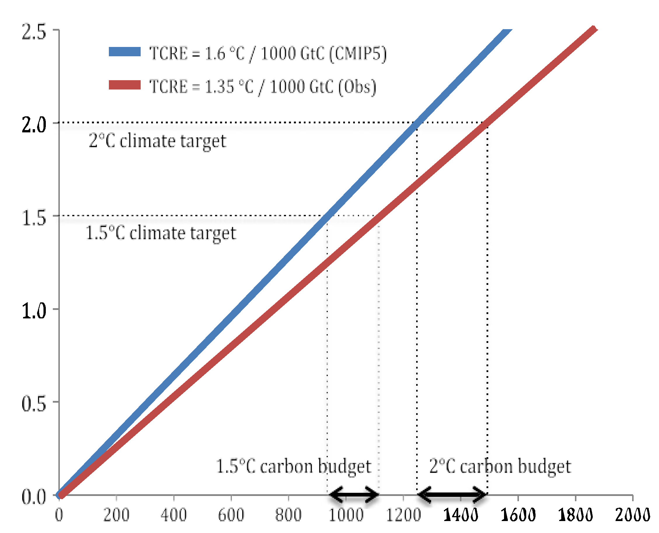
The global decarbonization rates towards 1.5 °C and other climate scenarios have been simulated in a previous study by Akpan J. et al. [22], in line with several other forecasts, research findings, and international energy reports, such as the ones in [5,23,24,25,26]. Low-carbon technologies are projected to contribute between 50% and 75% to scenarios with a budget below 1000 GtCO2 by 2050, with a >66% chance of limiting global warming to below 2 °C [27]. The carbon budget, determined by CO2 emissions, can be explained according to [21] by the relation in Equations (1) and (2) below.
where ec is the budgeted emissions, while ETCRE is the transient climate response to cumulative emissions (TCRE); both the ec and ETCRE are computed from observational data or Earth system models (ESMs) with a dynamic global carbon cycle and are represented by ΔE/Tr.
ΔE represents the cumulative emissions, while Tr is the global temperature rise over time. By reducing the cumulative emissions, the global temperature rise could be reduced as a direct relation, whereas an increase in the emissions moves the global temperature rise higher, as can be seen in Figure 1, showing the carbon budgets for the 1.5 and 2.0 °C climate scenarios. The amount of carbon dioxide released into the atmosphere throughout the Industrial Revolution is directly correlated to the increase in global average temperature that occurred during that time [28].
The goal is to achieve zero net emissions, as per the Paris Agreement; since climate change’s effects are already visible, low-technology energy must be employed to create fuels that could facilitate this need across all regions and countries [1]. The Paris Agreement includes provisions for countries to establish their targets for decreasing emissions of greenhouse gases through mechanisms known as nationally determined contributions (NDCs). These NDCs should be assessed for ‘fairness’ as part of a planned ‘ratcheting-up’ mechanism to guarantee they are in line with the larger aim of limiting the rise in world average temperature to far below 2 °C or even 1.5 °C [1,29,30].
In Figure 2a,b, fair rationing approach with an emissions reduction cap or rate was used in our recent study [22] to ascertain the emissions budgets towards the different climate scenarios at both the global level and country levels (USA, China, EU, and India), respectively.
Obviously, the mitigation targets for both the 1.5 and 2 °C scenarios, as shown in Figure 2a,b, would necessitate a very high global commitment of about 2.5 and 6% reduction in emissions from the current or baseline levels [22]. From Figure 2b, the 2022 baseline emissions combined value in only China (14.78 Gton CO2 eq.), the USA (6.93 Gton CO2 eq. CO2 eq.), EU (4.33 Gtons CO2 eq.), and India (4.55 Gtons CO2 eq.) is approximately about 50% of the 62.02 Gtons CO2 eq. global baseline, as shown in Figure 2a. Hence, as top emitters, emissions mitigation, as shown in the corresponding 1.5 and 2.0 °C scenarios of Figure 2b, would significantly help transition the globe to the desired climate scenarios of 1.5 and 2.0 °C (Figure 2a). Several other studies that have analyzed and proffered commitment pathways with carbon budgets globally and in these top emitting countries have also been investigated and are presented in Table 2. The carbon budget concept distributes global carbon across nations to keep emissions below 2 °C and equalize per capita CO2 emissions within decades [31].
Recent global carbon budget estimates—cumulative CO2 emissions consistent with a certain degree of climatic warming—may strengthen climate mitigation policy dialogues to keep world temperatures within the 1.5–2 °C range. However, this presents significant problems regarding how to distribute this carbon budget across nations to respect the finite cap on overall emissions and solve the underlying disparities across states in their history and future emissions. The inadequacies regarding the egalitarian, responsibility-based, right-based, and capability-based models of carbon budget sharing that have gained popularity in recent decades are highlighted by this study [31].
The rate of progress towards sustainable development goals by individual nations has been used as the major comparable indicator in an endeavor to distribute the global carbon budget fairly. Along with these factors and the climate action of each nation, Rawls’ idea of justice is applied to the allocation of the carbon budget [31]. The fair carbon budget share (FCB) model is a novel, dynamic, and prospective mechanism that is required for the annual distribution of countries’ carbon budget shares. From the studies, there were large discrepancies between countries’ actual carbon emissions and their fair share in both 2017 and 2018, and the shares determined using FCB were very different from the shares generated using the egalitarian method. The 2017 fair share, which revealed a solid equilibrium between debtor and creditor countries in relation to their actual greenhouse gas emissions, demonstrated that a market system can be prepared for implementation by the FCB model. Lee C. et al. [32] used the contraction and convergence method to show that a country’s cumulative carbon debt (or credit) is its past emissions compared to its share of the world population. This carbon debt/credit method simplifies setting national climate mitigation targets that account for past obligations and respect international equity in future emissions permits among countries.
An equitable approach to allocating the global carbon budget is explored in the study by Kanitkar T. et al. [33]. The paper makes a distinction between “entitlements to carbon space” and “physically available carbon space,” which is not always the case in previous treatments. All countries can apply the same mitigation strategy owing to the carbon budget approach detailed here. This method clearly operationalizes the notion of “equity and common but differentiated responsibilities and respective capabilities” to achieve climate goals [33].
The research by N.J. van den Berg et al. [34] assessed the feasibility of applying these criteria of fairness and equity to the formulation of national emission targets and carbon budgets. It found that industrialized nations may end up with (large) negative remaining carbon budgets, which can be achieved using either the equal cumulative per capita or the greenhouse development rights approach. All effort-sharing options for industrialized countries lead to more stringent budgets than cost-optimal budgets, and cost-optimal processes do not lead to outcomes that can be defined as fair.
The Paris Agreement has led to the EU’s ‘Fit for 55’ policy package, which includes ambitious strategies for reducing GHGs in all economic sectors. However, the issue of whether the planned policies are sufficient to keep global warming below 1.5 °C remains unresolved. The research calculates transport GHG budgets throughout the EU27 and obtains European GHG reduction plans sufficient for a 1.5 °C rise in global temperature. The analysis indicates that the “Fit for 55” campaign of the transport sector is not yet as ambitious as necessary to accommodate a 1.5 °C scenario [35].
In the study by O. Alcaraz et al. [36], 15 countries currently at the top of the global emissions ranking were studied. Initial investigation has revealed that only the intended nationally determined contributions (INDCs) of these 15 countries are assumed to release into the atmosphere 84% of the GCB between 2011 and 2030 and 40% of the GCB between now and the end of the century. A first attempt to use the System Dynamics-based FML model to generate city-level CO2 emission numbers for cities of varied sizes in Malaysia was carried out by [26]. To determine a city’s carbon budget, W.K. Fong et al. in [37] proposed three methods: equal share, population, and gross domestic product. The current model can accurately forecast historical, current, and future levels of carbon dioxide emissions from cities. Carbon dioxide emissions are generally on the rise, correlated with population and GDP [38]. Developing a national database of city-level CO2 emissions is one example of how this method could be used in Malaysia and other developing countries.
Other estimates of the carbon budget were examined by M. Dickau et al. [10], focusing on outlining significant uncertainties and evaluating their implications for climate policy and net-zero CO2 targets. This suggests being upfront about the degree of uncertainty surrounding carbon budget forecasts and suggests that these goals should be updated frequently. The idea is well-suited for guiding climate policy and determining if net-zero CO2 targets are consistent with the goals of the Paris Agreement according to new research into the carbon budget’s level of uncertainty. Despite these difficulties, the notion is still worth considering.
When considering that the world must be CO2 neutral by 2050 to achieve the 1.5 °C goal, the average amount of the global carbon budget used up by 2030 should not be more than 55 percent [38]. To keep global warming below a set threshold, scientists have calculated a “Global Carbon Budget,” or GCB. The empty GCB represents all of humanity’s historical emissions, most of which have come from industrialized nations. The remaining GCB is the sum of CO2 emissions that can be produced without risking a rise in the global average temperature above a predetermined threshold. The AR6 forecasts that, as of the beginning of 2020, 400 GtCO2 is the remaining GCB that is consistent with the Paris Agreement (PA) goal of limiting the global temperature increase to 1.5 °C [38]. This estimate is said to be more than 60% accurate [38]. To what extent a country uses its leftover GCB to implement its NDC and LT-LEDS is a key factor in determining the country’s national climate equity viewpoint [28].
Carbon pricing has also proven to be useful for both carbon budgeting and essential for abatement, encouraging economically viable high-penetration renewables. For instance, B. Elliston et al. [39] determined that a price on carbon was necessary for a completely renewable portfolio. The results showed that a carbon price of USD 50–65 per metric ton of CO2 equivalent (MTCO2 eq.) is required for a 5% discount rate. Also, a carbon price of USD 70–100/MTCO2 eq. would be required if the discount rate were raised to 10%. Replacement of older fossil-fueled generators with newer fossil-fueled ones is economically desirable when carbon costs are below this level [39]. The next section highlights studies across different countries and regions relating carbon pricing, carbon emissions budgets, marginal abatement cost and other indicators with climate scenarios.
2.2. Emissions Budgeting and the Use of Marginal Abatement Cost
Once a carbon emissions budget is known, the marginal abatement cost MAC (i.e., the cost needed to reduce a unit of CO2/ton of emissions) can be estimated. Marginal abatement costs play an important role in the allocation of emission reduction allowances and the planning of emission mitigation [40,41]. Several works, including a selected few such as the ones in Table 2, have dealt with the marginal abatement cost of emissions for different countries, with some aligning their investigations with different climate scenarios.

Table 2.
Related emissions mitigation planning and budgeting across selected countries and regions. Source: authors’ elaboration.
Table 2.
Related emissions mitigation planning and budgeting across selected countries and regions. Source: authors’ elaboration.
| Country | Study Summary | Method | Key Indicators | Climate Scenario | Ref. |
|---|---|---|---|---|---|
| World (For 41 regions, including 165 countries) | Emissions mitigation costs and their determinants were studied. The results showed that energy consumption, financial crisis, CO2 emissions rate, and GDP were great determinants and that, as the globe’s CO2 emissions continue to rise due to increasing GDP, reducing emissions is becoming more expensive | Gravity model and quadratic directional output distance function | MAC | No | [42] |
| Global | The different MAC methods used in climate change policy to evaluate alternatives and costs were comprehensively reviewed. The study classifies MAC techniques and presents an applicability path analysis for the estimation of MACs. The study suggests that complex methods may not always be better than simplified ones, and MACs could be more reliable by ranking the relative value of options. | Review | MAC | Yes | [43] |
| Global | The projected annual abatement costs of achieving national climate plans (NDCs) were estimated based on domestic action, land, land use change, and forestry (LULUCF) exclusion. The result showed conditions varying significantly across countries and achieving 2 °C being more expensive. | IMAGE integrated assessment model | MAC | Yes | [44] |
| China | A low-cost path for China to peak its carbon emissions was explored. For each region before 2030, it calculates carbon emission efficiency and marginal carbon abatement cost using the parametric directional distance function. Rapid economic expansion increases marginal abatement costs, with developed areas sustaining development patterns and central and western regions adopting emission reduction responsibilities. The work stresses that the current emissions reduction path may yield an increasing MAC in the future. | Parametric directional distance function | Carbon emission efficiency and MAC | No | [45] |
| China (441 industries) | The correlation between MAC and carbon intensity varies among industries, with energy-intensive industries showing a significant S-shaped relationship. | Functional data analysis | MAC, Carbon intensity | No | [46] |
| China and India | The costs and benefits of India’s and China’s NDCs were compared. It was found that India’s original carbon MACCs are generally higher than China’s, but revised MACCs are slightly higher. Yet, India has more significant cost-saving effects, while China faces difficulties in reducing emissions. | Computable general equilibrium model | MAC and CB | Only NDC Scenario | [47] |
| India | The study compares India’s National Development Goals (NDC) and global temperature stabilization targets, finding significant emissions disparities. Delaying abatement measures could increase mitigation costs. | Computable general equilibrium model | MAC | Yes | [48] |
| USA | The study examines the US climate policy’s costs and benefits, focusing on CO2 emissions levies and tax relief. Cost–benefit values vary from USD 150 to 1250 per household, while policy costs average less than 0.5%, demonstrating significant heterogeneity across space and income. The research shows a marginal welfare cost and cost–benefit of USD 31/tCO2 and a climate benefit of USD 27/tCO2 or less to justify a USD 25/tCO2 tax rise at 5%. | Computable general equilibrium model | MAC and CB | Yes | [49] |
| USA | The results showed that zero-carbon US electricity infrastructure would incur additional MAC, which can be reduced by employing low-carbon resources, and technologies with negative emissions show a financial benefit. | Sequential optimization model | MAC | Yes | [50] |
| EU | The paper analyzes the least-cost GHG emission abatement pathways in EU countries. A correlation was established between 2030 abatement objectives of varying ambition and a country’s probability of accomplishing a strong 2050 aim. | Constrained optimization model | Emission target, MAC | Only NDC Scenario | [51] |
| US, EU, China, and India, | According to the study’s hypothesis, nations with relatively low marginal costs of carbon emissions could end up paying an enormous cost to combat climate change. The analysis estimates the total and marginal costs of abatement for the US, EU, China, and India based on the outcomes of the 22nd Energy Modelling Forum. | EMF-22 models | Emission target, MAC | Yes | [52] |
| EU | This study explores decarbonization possibilities that combine energy systems analysis with marginal abatement cost curves (MACs). The findings indicate that MACs rely on model assumptions, with bioenergy and CCS technology being important factors. Important mitigating actions are categorized into three groups: resilient, tipping-point, and niche. | A novel analytical technique | Energy System Analysis, MAC | Only NDC Scenario | [53] |
| Developing countries | This study examines developing nation emission goals, abatement costs, and energy use in 2020. The findings showed that, by 2050, developing nations would have tougher emission objectives and higher abatement costs. | Integrated modelling framework FAIR | Emission targets, MAC, and energy consumption | Only NDC Scenario | [17] |
| World, China, EU, India, and the USA | This study examines the emissions targets from 2023 to 2050 under the climate scenarios for the World, China, EU, India, and the USA. The results show the comparative time values of different investment decisions towards the selected climate scenarios. | Developed in the Study (a simplified budgeting model approach) for evaluation of the attractiveness of emissions investment policies | MAC, NPV, CB, Avoided Emissions Cost Growth | Yes | This study |
2.3. Rationale of Emissions Budgeting (EB) Model
The research reviewed in Section 2.2 and Table 2 has provided a foundation for understanding MAC and its relation with climate scenarios for countries and the world. Most research is just like that highlighted in Table 2, hardly discussing the economic attractiveness of the climate scenarios in a quantifiable manner. Given the marginal abatement cost, potential investment opportunities can be weighed [40,41]; hence, evaluating the attractiveness of potential investment options can also be completed. Therefore, this study uses a simplified MAC to estimate avoided and unavoided emissions costs (explained better in the next Section Methodology) to guide in understanding the attractiveness and viability of an investment or policy choice towards reducing the GCB for countries/regions and the world under the climate scenarios. In determining the attractiveness of each policy scenario, the principle of capital budget is incorporated.
Generally, capital budgeting techniques (CBTs) are used to determine the most attractive option for making investment decisions. CBTs are often determined mainly through two categories; the first is based on discounting criteria constituting the net present value of investments NPV (value of investment at current time), internal rate of return IRR (return on investment), and profitability index PI (profit ratio for every unit of money spent). In contrast, the second is based on non-discounting criteria such as accounting rate of return ARR (returns on investment after tax and depreciation) and payback period PBP (time to recover the investment). Figure 3 shows these categorizations. Since CBTs are a planning choice, these indices affect both the predictability of the budget and the actual spending.
Capital budgeting techniques (CBTs) indices shown in Figure 3 have been extensively discussed and referenced in the literature, some of which include the ones in [54,55,56,57] and with a five-decade review on CBT by Sureka et al. in [54]. Pintarič, Z. et al. in [58] emphasized the significance of understanding the application of CBTs. Sureka et al. [54] concurred that the utilization of modern methods, such as discounted cash flow (DCF), yields higher capital investment and eventually contributes to enhanced long-term profitability. It is generally accepted that the NPV is the favored index among researchers since it measures the potential financial gain from selecting the best alternative [54].
The internal rate of return (IRR), despite NPV, is also used in business because it enables more detailed comparisons of projects of various sizes by utilizing a single rate of return that is unaffected by the discount rate [54] and may become erroneous if the project is mutually exclusive [59]. In this study, NPV is preferred for use as each policy scenario begins with the same amount of emissions to be removed, and comparison is only made against the best-case scenario (i.e., the 1.5 °C scenario). The discount rate is also varied based on the prevailing global inflation rates and GDP growth in each investment scenario.
Žižlavský in [56] demonstrated the potential financial value of the NPV method to the management of innovation projects. Pintarič, Z. et al. [58] stressed the importance of NPV as an economic criterion that can provide design compromise with intermediate efficiencies and impacts, such as environmental benefits, when profit consideration may be less attractive. When examining the time worth of money, sustainability net present value results from the trade-off between economic profitability, environmental (un)burdening, and social benefits like the creation of new jobs [57]. With the results that are obtained from the budgeting indices, an investment decision can be made by the following evaluation rules, shown in Table 3.
CBT practices have been applied even at organization and country levels for improved decisionmaking. The summary of the findings from the use of CBTs is presented in Table 4.
The studies reviewed in Table 4 confirm the greatest acceptance of the use of DCF analysis techniques (most particularly the NPV method) for large investments. However, the choice and use of analysis techniques appear to be independent of the type of project being evaluated, with no significant difference between the use of techniques for strategic and non-strategic projects. Risk analysis techniques, such as sensitivity/scenario analysis, probability analysis, computer simulation, and beta analysis, are more often used for strategic projects, suggesting that strategic projects would require greater attention to risk issues [67]. Only two of the CBT practices explored across the studies reviewed in Table 3 have also attempted to incorporate scenario analysis to understand and assess the risk of investment decisions. For instance, the CBT practices study for the Fortune 1000 companies by Ryan P. and Glenn P.R. in Ref. [59] and that of the Pakistani firms by Mubashar A. and Bin Y. in Ref. [62] attempted the incorporation of scenario analysis.
Therefore, in addition to the scarcity of studies in the literature on the use of NPV and scenario analysis to evaluate capital investment decisions, an empirical analysis of direct integration and balance between strategic investment decisions and financial analysis approaches is pertinent.
Hence, in this study, the use of NPV is adopted and synthesized for the scenario analysis of different policy options aimed at mitigating emissions towards different climate scenarios at the global level and in four countries (i.e., China, the USA, the EU, and India). The methodology developed is described in the next section of this study, Section 3.
3. Methodology
3.1. Overview
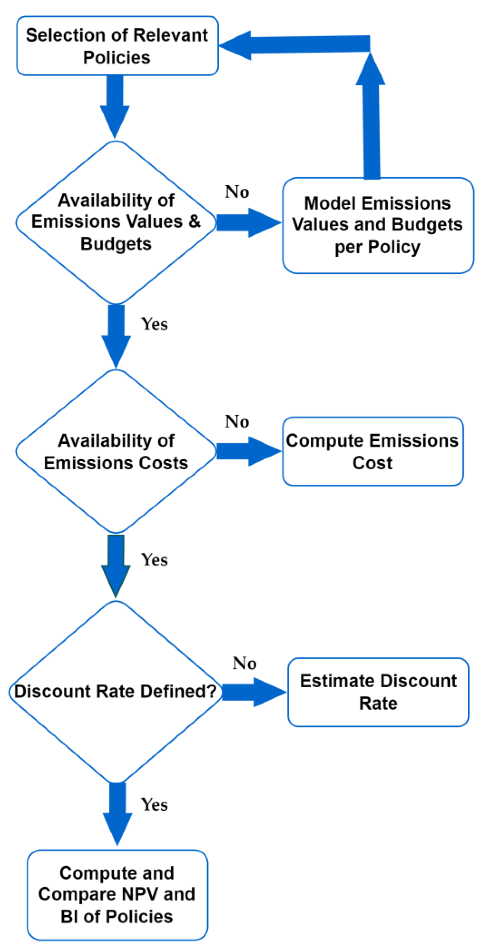
The proposed simplified framework for performing the investment attractiveness of emissions budgets is shown in Figure 4. The emissions budget datasets are projected against the climate policy scenarios. Using the CBT indices to calculate the economic maximization and attractiveness, the cost–benefit analysis is then evaluated for all the climate policy scenarios by considering the framework of Figure 4, which is explained further through the emissions budgeting (EB) modelling process of Figure 5.
Additionally, this EB model conducts the cost–benefit analysis in terms of NPV, BI, and avoided emission growth rate among the climate policy scenarios, providing a better understanding of the time value of the policy. The results are then validated to establish the relationship between delayed policy economic attractiveness to allow for a more comprehensive understanding of the economic risks and benefits of climate policy options.
3.2. Model Inputs, Assumption, and Computation Strategy
According to the global energy outlook by IRENA in [68], the current investment trajectory needs to be maintained through 2050 with an additional cumulative investment of USD 47 trillion to stay within the 1.5 °C scenario. This sum is in addition to the USD 103 trillion in investments anticipated under the Planned Energy Scenario (herein announced policies type 2 in this study). In this part, both the announced policies type 2 and the 1.5 °C scenario finance requirement were used to estimate the requirements for the other three scenarios, as shown in Figure 4 and with the financial requirements shown in Figure A1 alongside Table A1 and Table A2.
3.3. Selection of Relevant Policy Scenarios and Corresponding Emissions Budgets
In the report by IEA in [5], three forward-looking scenarios (net-zero, SDG, and stated policies) were defined and used to provide a landscape for clean energy financing in emerging and developing economies. The net-zero, SDG, and stated policies scenarios were compatible with approximately 1.5, 2.62, and 3.0 °C climate scenarios defined in this study. This study includes additional scenarios, as shown in Tables S1 and S2, to present the economic viability and value of each policy option at the global scale, as well as for the top emitting countries. The emissions values of each policy used have been defined in Table S2.
3.4. Categorization and Monetization of Emissions
The financial investment requirement cost set for the best-case simulated policy scenario (i.e., 1.5 °C scenario) serves as the base cost for comparison of benefits with other policy scenarios. In order to calculate the unit base emissions cost (i.e., the marginal abatement cost), the following assumed relations in Equations (3) and (4) are applied.
where ebc is the unit base cost of emissions removal (USD trillion/Gtons CO2.eq/year) and ei is the initial i emissions value (Gtons CO2.eq/year) at the start year of the policy. Ce1.5 is the best case (i.e., 1.5 °C scenario) cost in USD trillion. Hence,
Therefore, a unit of Gtons CO2.eq represents USD 2.42 trillion, which herein represents the financial requirement to remove 1 Gton of CO2 eq. emission. Notwithstanding the heterogeneity in the determination of the MAC option [40], a comprehensive review study on the applicability of MAC by Huang S. et al. [43] suggested that complex methods for MAC estimation may not always be superior to simplified ones as policymakers must choose the right method for specific information needs. Hence, the study adopted the simplified Equations (3) and (4) to estimate the unit base cost of emissions removal.
Here, eac is the avoided emissions cost for each n year, n = 1, 2, 3, …, 27, for (2023–2050). Cen is the financial investment requirement for the number n of different scenarios (i.e., baseline, announced type 1, announced type 2, 2.0 °C, and 1.5 °C scenarios), cost in USD trillion.
Annual emissions flows and their monetary values are crucial to industrial and environmental economics and climate change policy analysis. They enable policymakers to evaluate the viability and consequences of climate policies by quantifying the economic costs and benefits of various policy options. This method is useful in pinpointing the best methods for reducing greenhouse gas emissions at the lowest possible cost. In this part, the economic impacts of various financial requirements and the resulting emissions values towards the 1.5 °C scenario are assessed by assigning monetary values of the climate policy scenarios.
Similarly, Equations (3) and (4) were employed to estimate and assign the unavoided and avoided emissions cost per policy at a time throughout the period, as shown in Equations (5) and (6). The outcome of the unavoided and avoided emissions cost estimated are presented in Tables S3 and S4, respectively. Then, Equations (5) and (6) are used to compute the NPV as in Equations (7) and (8) for each of the policy scenarios based on the input parameters.
The relation of Equation (9) is adapted from the concept of calculation of profitability index in cost–benefit analysis estimation, a measure of investment’s attractiveness, where NPV is the net present value of the capital for a selected investment option or financial requirement I.
The BI is then determined by using Equation (10), where NPV is the net present value of a selected policy scenario, determined by the relation of avoided emissions cost and the emissions discounting rate, R, over the investment period, t. This R-value (i.e., discount rate in capital budgeting) has no universal formula; rather, it can depend on the prevailing situation, for instance, high inflation rate, investment cycle, and a host of other factors.
To be able to obtain R, the possible growth rate of GDP from the different investment scenarios is used as depicted in Tables S5–S9. An average GDP growth rate for the specified period (between 2023 and 2050) of CB analysis was used as input for the discounting emissions cost flow rate calculated using Equation (11) in this study.
where N is the number of periods or simulation years, tf is the average GDP growth rate at the last year, and ti for the initial year.
3.5. EB Model Fitness
In Table 5, P1, P2, P3, P4, and P5 represent the values of the emissions cost discounting rate for the baseline, announced policies types 1 and 2, 2.0 °C, and 1.5 °C scenarios, respectively. The computation of the P values is included in Tables S5–S9.
Equations (12) and (13) are utilized to assess and interpret the available data for use as emissions cost discounting rate (R) per policy p, considering the anticipated that an increased global real gross domestic product (GDPavr) would result in R increase.
The symbol d/dt represents the derivative of a GDPavr variable with respect to time in years. The equation demonstrates a positive correlation between the growth rate of GDP and the discount cost for emissions reduction per policy option P1–P5, as indicated by the proportionality ∝.
Rp is expected to vary depending on the policy scenario P, but it cannot go above a specified limit max (Rp) = 3% as the global GDP growth rate is forecasted to be between 2.5–3% by 2050 according to the OECD data in [69]. Hence, only three cases are used in this study to keep the emissions cost discounting rate less than 3%, which is assumed with the GDP growth rate.
When contemplating the implementation of a policy scenario in the anticipated first year, it is crucial to acknowledge that the amount of investment required may vary if it is postponed to a different year. This consideration should take into account potential risk variables that might have either negative implications, such as inflation, or positive implications, such as technological breakthroughs and cost reductions.
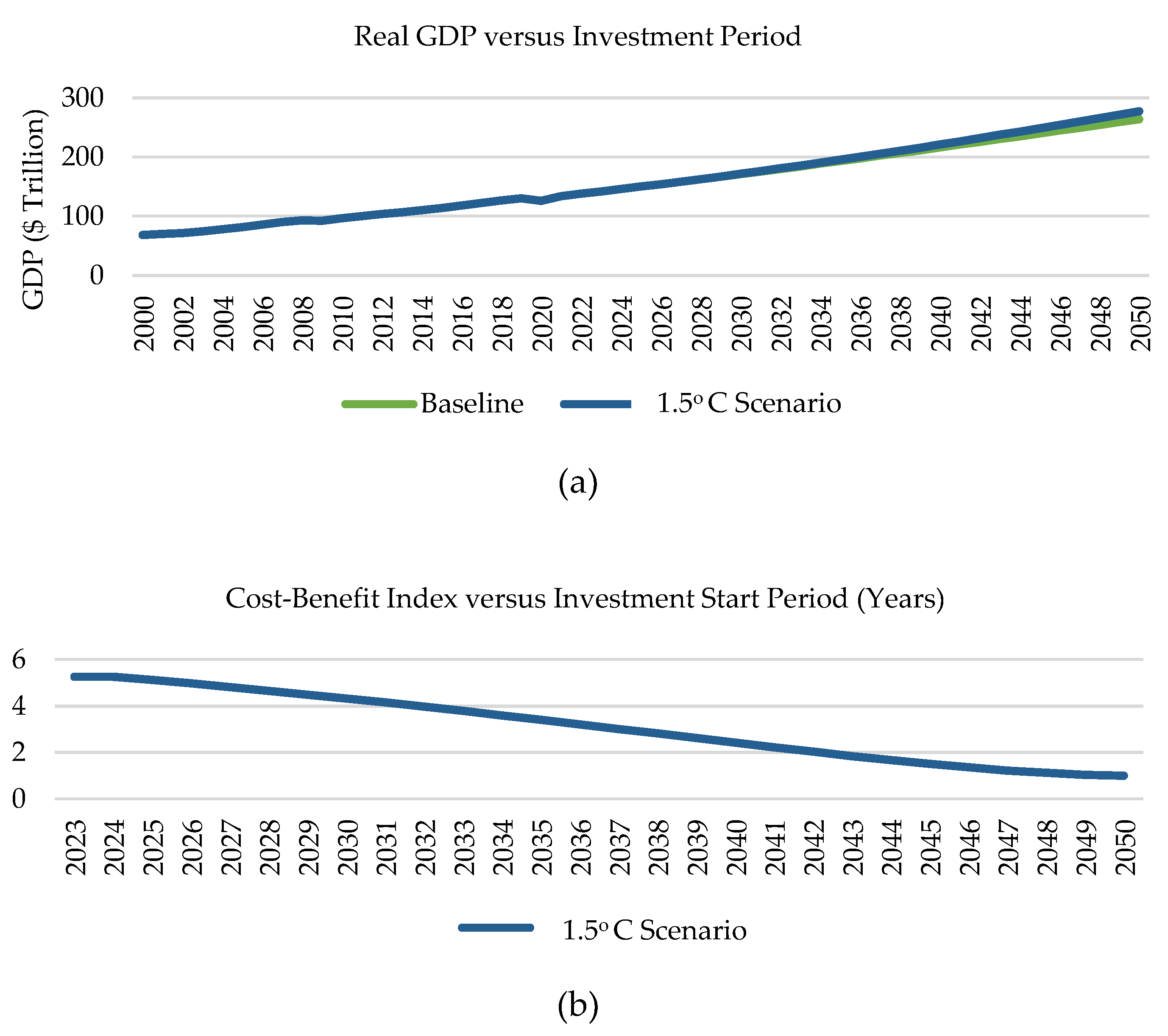
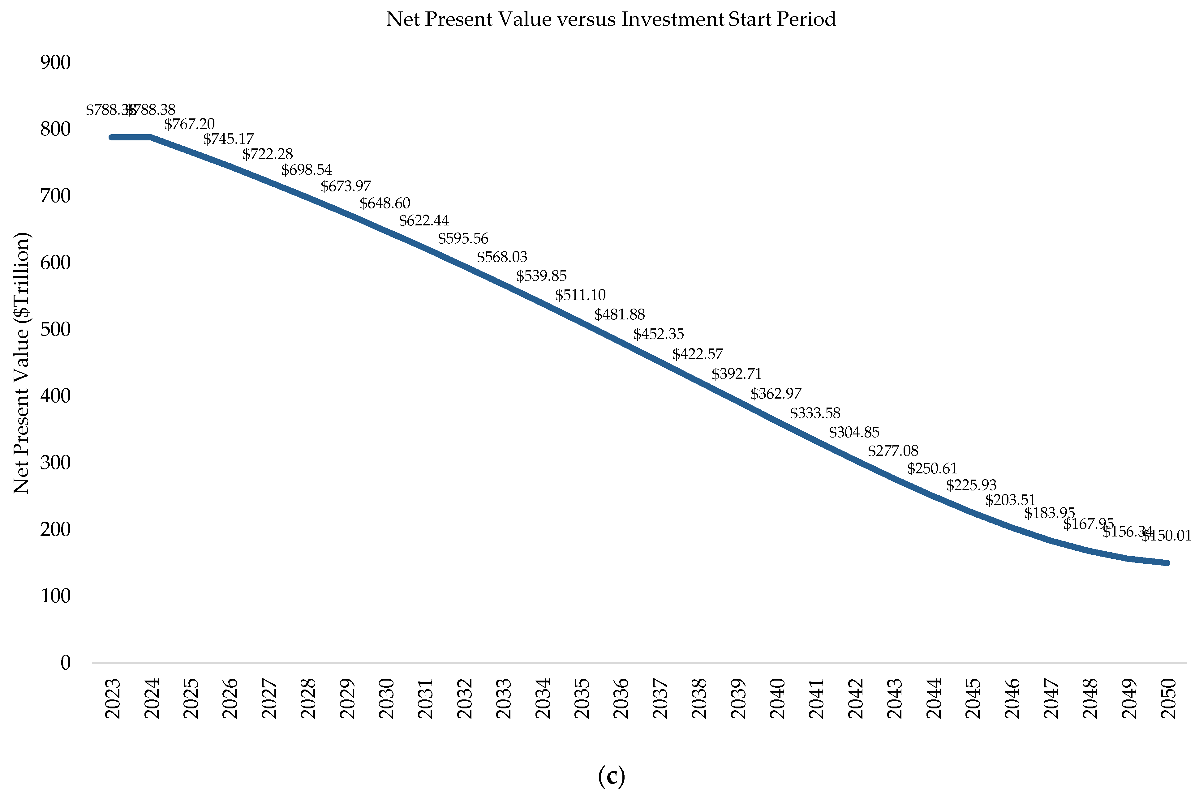
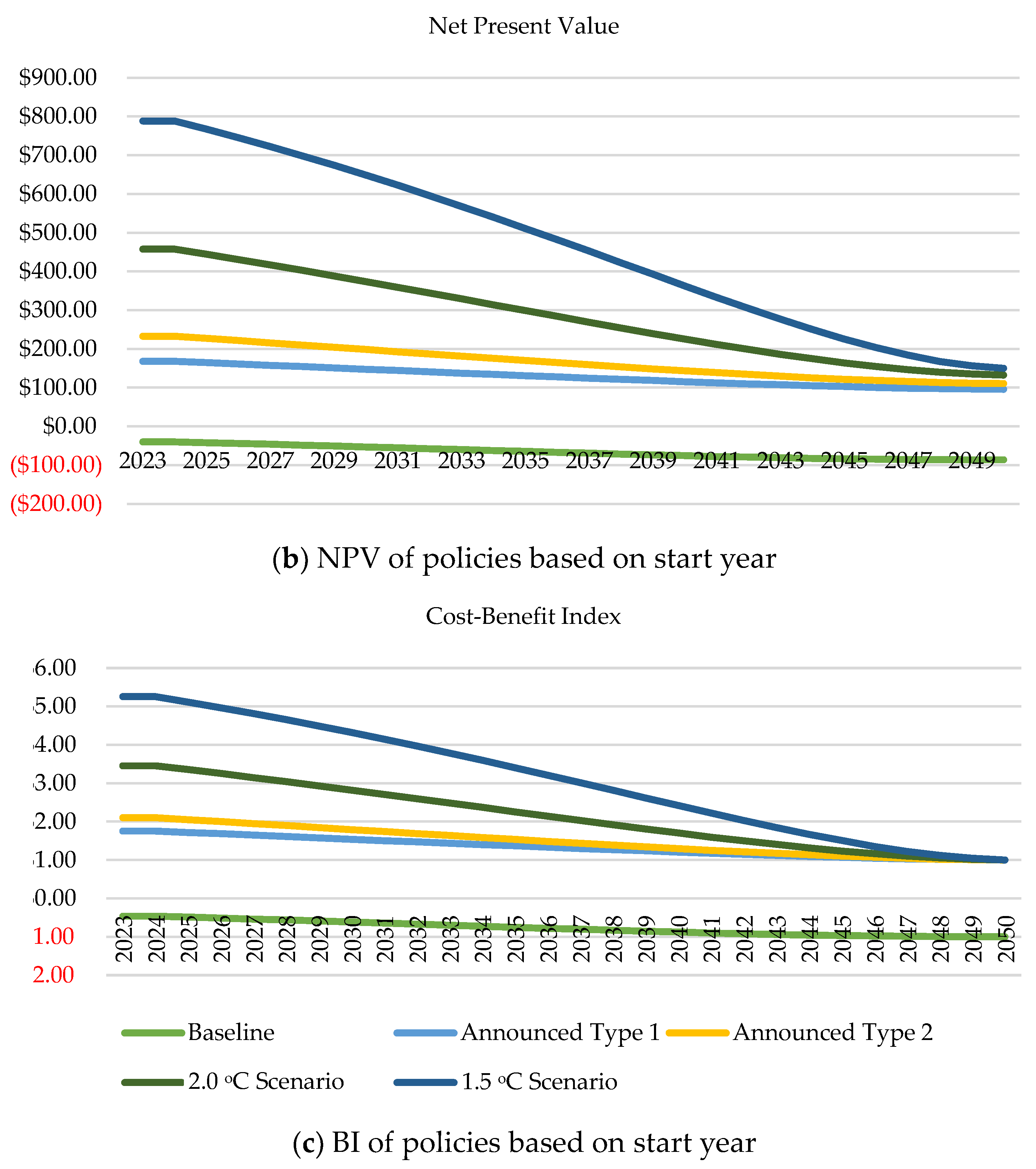
Given the focus of our investigation on climate change risks, it is unlikely that a delayed investment would provide any favorable benefits. Consequently, the net present value of an investment made in a subsequent year to attain an equivalent policy scenario is hypothesized to drop, hence Equation (14). The best case (i.e., 1.5 °C scenario) data shown in Figure 6a–c are used to establish and fit the model that assumes a reverse correlation between the emissions cost discounting rate (R) and the net present value (NPV).
4. Results and Discussion
4.1. Results—Global Policy Scenario
Figure 7, Figure 8 and Figure 9 show the outcomes of the NPV, avoided emissions cost growth, and cost–benefit in the three different cases and are explained accordingly.
Case 1: Use of the initial emissions cost discounting rate.
Figure 7, Figure 8 and Figure 9 show the different policies’ financial requirements, with the outcome of the NPV and avoided emissions cost growth when the discount rate per policy is between (2.29–2.48) %, (2.52–2.73) % and (2.64–2.85) % for cases 1, 2, and 3, respectively, and with reference to Table 4. In the baseline scenario of case 1, the NPV is USD −33.99 trillion, showing that the value of emissions commitment in the first year of 2023 is not useful, and, hence, such investment would not be suitable for mitigating emissions.
In the other four scenarios, the NPVs are USD 174.05, 243.06, 485.08, and 841.22 trillion for announced policies type 1, announced policies type 2, 2.0 °C scenario, and 1.5 °C scenario, respectively. As with case 2, the base scenario has an NPV of USD −38.12 trillion. Hence, this shows that the value of the emissions pledge in the first year of 2023 is not useful, so it is insufficient to reduce emissions. For stated policies type 1 and announced policies type 2, the NPVs are USD 168.02, 232.75, 457.66, and 788.38 trillion, respectively.
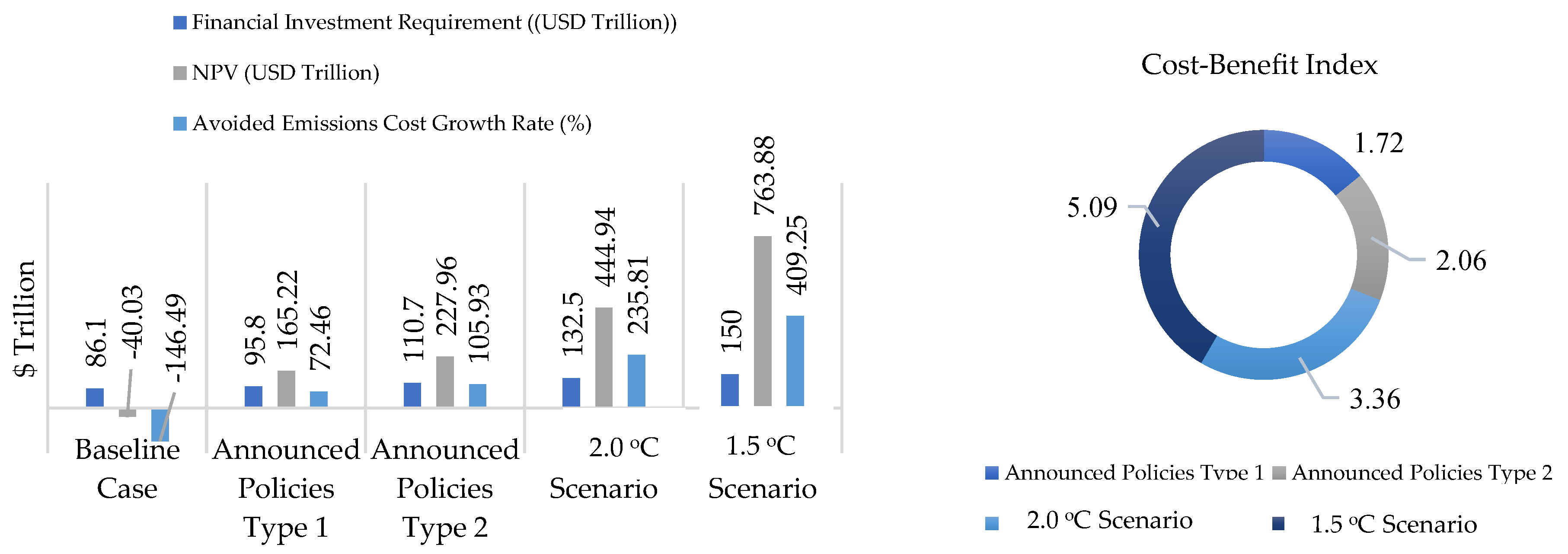
Similarly, case 3 produces an NPV of USD −40.03 trillion, with 165.22, 227.96, 444.94, and USD 409.25 trillion for the respective four scenarios. As can be observed from the results, the NPV reduces with an increase in the discount rate from case 1 to case 3, which is in line with the well-known fact that the NPV of investment diminishes with an increasing discount rate [70,71]. Therefore, this is in line with the work by Wang Z. et al. [72], which presents that the unit cost of emissions removal would likely increase in the short term. This could be attributed to inflation and the possible increased cost of financial requirements to meet an emissions mitigation target. The study by Liu J. and Feng C. [42] reveals that increasing financial costs, CO2 emissions mitigation rate, and GDP are significant determinants of emissions mitigation costs, with rising GDP making reducing emissions more expensive.
While the financial commitments in the announced policies type 1 and announced policies type 2 have been able to reduce the emissions growth rate and have positive NPVs, this is still insufficient to reach the 1.5 to 2.0 °C scenarios. An earlier study by Akimoto K. et al. [73] analyzed the economic costs of achieving NDCs and expected global emission pathways of 1.5 and 2.0 °C. The study found that emission reduction costs vary widely among countries, leading to carbon leakage. Our study has provided further analysis of the NPV and BI of these pathways, as well as the time value of policy decisions used to validate our model, as discussed in Section 5. The expected global emission reduction is smaller than predicted by aggregating reductions, and emissions are larger than those required for temperature stabilization, as suggested by the same studies [73].
The effectiveness, efficiency, uniformity, and equality of carbon allocation and emissions mitigation towards the desired global temperature scenarios continue to be a challenge, with the suggestion of preferences for utilitarianism–egalitarianism trade-off [74], national renewable expansion, and sectoral reduction targets at the level of municipalities [75], equitable energy demand reduction [76], and assessment of remaining carbon budgets’ size and uncertainty. The work by Fyson C. [77] suggests fair-share outcomes for the top emitting countries, the USA, EU, and China, which could result in 2–3 times larger CO2 mitigation responsibilities and in line with this study, which demonstrates possible costs and economic risk reduction, given early policy action.
The debate on equitable mitigation contributions is crucial for progress and in the assessment of more equitable economic costs by employing the model developed in this study. As part of an attempt to address this challenge, Hales R. and Mackey B. in [78] presented a perspective of equity in the carbon budget regarding the scale of achieving the Paris Agreement global temperature goals. In a follow-up study, Akpan J. et al. [22] employed a fair sharing approach in simulating the emissions budgets of the same USA, EU, China, and, in addition, India’s transition into the 1.5, 2.0 °C, and alternative scenarios. The emissions budgets, which are in line with the philosophy of Zimm C. et al.’s [79] recent work on justice consideration for climate change mitigation research, were then used in assessing the economic attractiveness and benefits, as presented in Section 4.3.
Comparing the differences in the benefits from each scenario as shown in Figure 7, Figure 8 and Figure 9, the 1.5 °C scenario has a very high benefit of 5.09 in relation to 3.36, 2.06, and 1.72 regarding the 2.0 °C, announced policies type 2 and announced policies type 1 scenarios. The baseline scenario has a negative benefit, and, as a result, such an investment venture should be highly rejected, in accordance with Table 3.
Similarly, the avoided emissions growth rates among the five scenarios and three cases depreciate with increasing discount rates. These differences are compared in Figure 10 below.
4.2. Illustrative Application of Emissions Budgeting Model to Other Cases
The results from Section 4.1 in the global policy scenarios show that achieving a transition to emission budgets in line with the desired climate scenarios requires investing in unprecedented financial commitments globally. However, these efforts must not only ensure a collaborative commitment but also target a significant reduction in emissions from the top global emitters. China, the USA, India, and the EU are the major emitters of CO2, and reducing current carbon in the atmosphere as well as committing to the reduction in further emissions from these countries and regions could highly facilitate the transition of the world into a net-zero society.
Consequently, the global energy investment report was developed in the current year of study by another IEA report [2]. In line with other separate energy and climate investment reports, Table A3 presents a summary of the financial requirements in both the planned (herein 2.65 °C) and net-zero scenarios (herein 1.5 °C) for China, the USA, India, Europe, and the rest of the world. These values are, therefore, going to serve as the input data to estimate the indices for the emissions budgeting model developed in this study.
The avoided and unavoided emissions costs are obtained to allow for the estimation of the budgeting indices. Two assumptions are introduced as described in Table 6 below.
Therefore, based on Equations (3) and (4), the unit base cost of emissions removal, avoided, and unavoided emissions costs are estimated. Also, the emissions cost discounting rate average GDP growth rate was calculated based on Equations (12) and (14), with the input data from the individual year GDP projection data obtained from OECD [69]. The GDP projection, which includes long-term baseline forecasts until 2060, is produced from an analysis of national and international economic conditions. This assessment is carried out by combining model-based analysis with experts’ opinions. This metric is often calculated in USD using 2010 constant prices and Purchasing Power Parities (PPPs).
4.3. Results–Other Cases
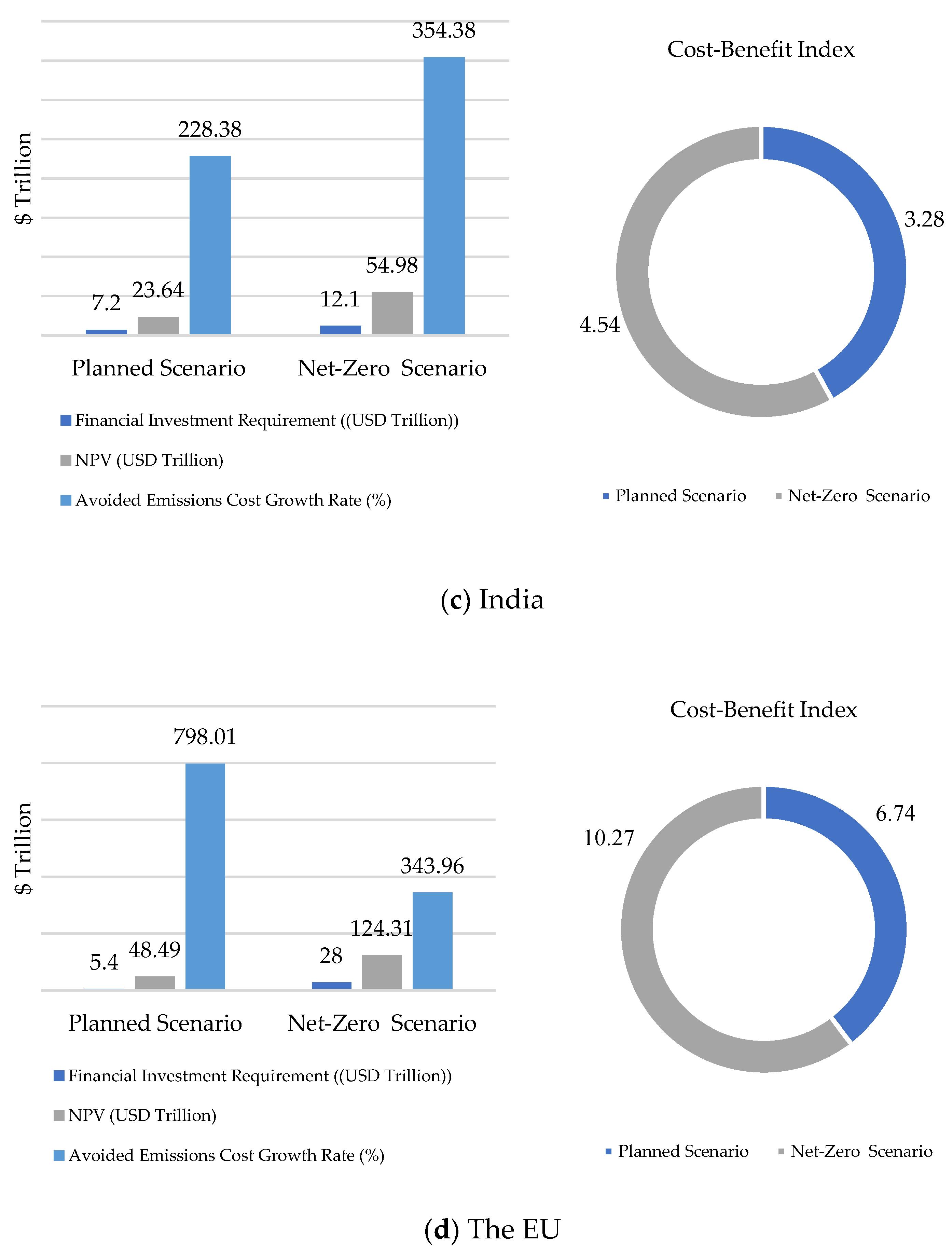
With the use of Figure 11a–d, this section presents the NPV, avoided emission cost growth, and cost–benefit findings for China, the USA, India, and the EU for the year 2050 at discount rates according to Table 5.
Figure 11a–d shows the financial requirements, with the NPV and avoided emissions cost growth with the corresponding cost–benefit index for the same countries, respectively, for China, the USA, India, and the EU.
In the planned scenario, except for the USA with USD −52.61 trillion, the NPVs of the financial commitment for emissions reduction are all positive for China, India, and the EU, with corresponding values of 35.78, 23.64, and USD 48.49 trillion, respectively. Therefore, the current commitment in the USA has to be increased as continuously following the baseline scenario is highly insufficient to reduce emissions regarding the net-zero scenario.
Following the net-zero scenario, all the countries showed a positive NPV, with China, the USA, India, and the EU having USD 107.65, 55.17, 54.98, and 124.31 trillion, respectively. Meanwhile, the commitment across each of the other four countries yielded NPVs that are not directly proportional compared with all the countries in both the planned and net-zero scenarios. These differences can be explained in Figure 12 with the avoided emissions growth rate across the four countries and two scenarios in each.
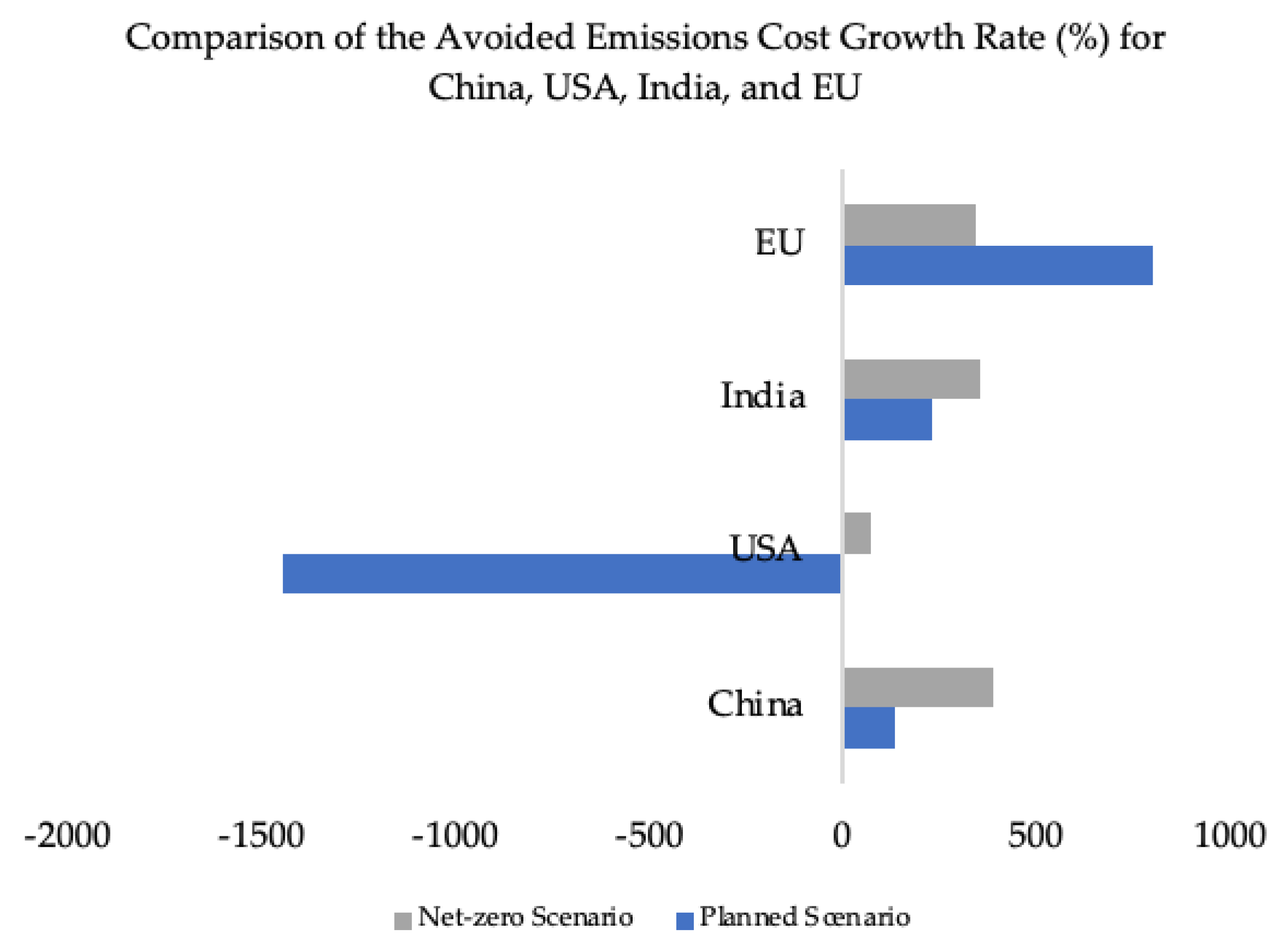
In terms of comparing the avoided emissions growth rates among the planned and net-zero scenarios in the four countries, Figure 12 shows that the rate of reduction from the net-zero investment results in the highest reduction in emissions compared with the planned scenarios. The planned scenarios showed that the USA would likely have an increase in unavoided emissions rate of −1442.18%. The implication is that the financial commitment is insufficient given the USD 2.4 trillion global unit emissions removal cost.
Furthermore, although the NPV in the EU is higher in the net-zero scenario than the planned scenario, the avoided emissions cost growth rate in the planned scenario is rather higher than in the net-zero scenario because the financial requirements estimated for the actual planned scenarios and the reported financial requirements for the net-zero scenarios in the EU may have used different unit costs for removing a unit ton of CO2, hence resulting in the differences as in this study as a single value was used across the four countries to avoid the differences that have been acknowledged in the literature [80,81] that the cost of removing (i.e., using low-carbon and net-zero technologies, carbon capturing, and sequestration of a unit ton of CO2) varies across industries and countries. Therefore, these approaches for carbon budgeting and emissions mitigation are not without implications and impacts, which have been discussed by N.J. van den Berg et al. [34,82]. Hence, insights for further investigation are presented for the use of the different unit costs of emissions abatement based on more precise values to better explain such occurrences in detail. On the other hand, even more important are the development and utilization of novel technology for emissions removal at lower costs [73].
While the financial commitment in the planned scenario of the case study countries has been able to reduce the emissions growth rate and have positive net present value except for the USA, the net-zero scenario continues to be the best pathway to follow towards reaching the 1.5 to 2.0 °C scenarios since these four countries have continuously been the major global emitters.
Comparing the differences in the benefits from each scenario, as shown in Figure 11a,c,d, the net-zero scenarios for China, India, and the EU have the best benefits of 4.89, 4.54, and 10.27 in relation to 2.34, 3.28, and 6.74, respectively, except for the USA, with no benefit (i.e., the BI value is −13.42) in the planned scenario and 3.03 in the net-zero scenario, as shown in Figure 11b.
5. Model Validation and Limitations
In order to validate the model, the time value of each policy scenario using the principle of capital budgeting through the net present value and cost–benefit of each policy is carried out in this section. The fitness model in Equation (14) shows that delayed policies result in a net present value and cost–benefit that may be different from using the same initial financial requirement to start implementing from the first year as planned. Hence, in the model validation, using the same initial financial requirement, the start of the policy implementation is delayed to the succeeding year, and that is completed continually until the last year. For instance, in the 1.5 °C scenario, the investment that was meant to start in 2023 was started in 2024 using the same initial financial requirement. Also, the envisaged GDP of each policy option used in estimating the emissions values was used in estimating the emissions cost discounting rate based on Equations (12)–(14), as shown in Figure 13a. After that, the emissions cost discounting rate was employed to calculate the NPV of each policy at delayed investment.
The model showed that the NPV and BI values on each policy option depreciated as compared to starting the investment in the first planned year. The results in Figure 13b,c showed that, with increasing delay in policy implementation, the BI and NPV of the initial financial requirement continue to diminish in the succeeding years at an increasing GDP.
The outcome of this validation is in line with real-world cases where an increasing GDP often leads to inflation and an increasing cost of capital to execute projects that should have been completed earlier on at a lesser cost. This study by Tørstad V. et al. [83], which evaluated the degree of ambition for mitigation under the Paris Agreement and the effects of various drivers across 170 nations, also confirms that GDP changes negatively affect NDC ambition. Hence, a country’s degree of responsiveness to early mitigation of climate change has economic value benefits. Therefore, GDP projected values should guide the planning of national climate ambition drivers.
Since the dangers associated with climate action are expected to rise over time, the time value of policy scenarios from the previous section shows that delaying action to reduce greenhouse gas emissions would be counterproductive and less economically attractive. The transition to keep Earth within the 1.5 °C climate scenario has been explored and is deemed to be doable by a number of publications and papers, such as the ones in [84,85,86,87,88,89], which look at the technical feasibility of accomplishing the climate objectives and achieving sustainable development. However, the challenge has often been viewed as mainly financially demanding [6,8,21].
In the evaluation of the financial requirements of the policy scenarios through this study and in the findings from Section 4.1 and Section 4.3, the economic benefits of the 1.5 °C climate scenario cannot be overemphasized. Considering this, it is clear that cutting emissions today is far wiser than waiting, and more financial regulatory mechanisms are needed because of the possibility of catastrophic losses due to climate change [15]. If all countries and regions were to stop emitting CO2 this year, the environment could benefit next year and every year after that. Meanwhile, if some regions were to start cutting emissions in 2030, the global carbon budget would have been drained for another extended period, making it unlikely that we can meet the 1.5 °C scenario.
In terms of environmental cost advantage, the value in terms of time for following the 1.5 °C scenario can be obtained immediately and before 2050 as the climate change consequences of further damages are averted through the reduction in emissions concentration in the atmosphere. Since CO2 has had a warming effect on the planet over decades, it is important to think about carbon stocks and fluxes in the atmosphere when planning for emissions mitigation. Both regional or countries’ non-uniformity in the reduction goals and continuing to follow the current paradigm of climate goals without swift action are detrimental because the required path to the 1.5 °C scenario is already over-ambitious; hence, it is rare to find regions exceeding the simulated 1.5 °C scenario reduction goal to create a balance for the deficiencies of other countries. As with the case regarding climate actions, environmental needs are very important as failure to mitigate the consequences can be more catastrophic.
The consequences of inaction might be disastrous; therefore, now appears the best time to act. Since CO2 has had a warming effect on the planet over decades, it is important to think about carbon stocks and fluxes in the atmosphere, hence shifting into swift action regarding high financial investment with cost–benefit analysis. The energy requirement and current cost for emissions capture are high and vary across countries due to differences in storage location, high design complexities, and customization needs. However, the future unavoided emissions costs could be decreased if initiatives and emissions capture technologies’ costs are also reduced. However, such breakthroughs are yet to happen; hence, the timeliness of deciding in the present is pertinent.
Despite the study’s useful insights regarding the economic importance and attractiveness of emission reduction policies, it is important to acknowledge the limitations and weaknesses in the study’s design and execution when interpreting the results.
This study may not be representative of the world at large because it focuses on just four countries—China, the United States, India, and the European Union, and the global level without the peculiarities of other individual countries. Therefore, the results may not absolutely apply to other countries or regions. Additionally, the study assumes that emissions mitigation policies would be implemented according to the planned timeline, which might not match up with the real situation. The study disregards the potential challenges and constraints to policy implementation, which may affect the economic attractiveness of such policies.
Also, the study does not take into consideration how emission reduction policies could affect society and the environment. The study does not include a detailed and thorough understanding of the policies’ overall consequences since it solely considers the economic benefits and risks. Consequently, some complexities in emissions mitigation policies were not adequately incorporated by the study’s simplified emissions cost budgeting model. Hence, the accuracy of the results and the conclusions derived from them may be influenced by the assumptions and limitations of the model.
6. Conclusions, Policy Implications, and Recommendations
The EB model from this study helps to analyze the investment attractiveness across the different policy scenarios. The results from the policy scenarios show that a small difference in financial investment options aimed at mitigating emissions could lead to a large cost–benefit difference, such as the following:
Economic Benefits:
- In the global scenario simulation and at the first case of no emissions discount growth, the 1.5 °C scenario achieved a higher NPV of USD 841.22 trillion and BI of 5.6, with an initial investment requirement of USD 150 trillion, compared with the 2.0 °C scenario having an NPV of USD 458.08 and BI of 3.66, yet with the initial financial requirement of USD 132 trillion. The baseline scenario resulted in negative NPV and BI, hence showing the consequences of the world continuing with the business-as-usual approach to emissions reduction. Meanwhile, the announced policies types 1 and 2 yielded positive NPV, implying that such investments could create economic and social benefits. However, it is not adequate to keep the world within the IPCC’s desired temperature levels.
- In the illustrative case studies, according to the model’s estimation in Section 4.2 and results of the illustrative application of the model to China, the USA, India, and the EU in Section 4.3, investment options towards the global temperature rise show that, apart from the environmental advantages of the 1.5 °C and net-zero scenarios, the present economic value is also very high compared with the other scenarios. In all the planned scenarios for China, India, and the EU, the emissions reductions achieved are insufficient to meet the net-zero scenario target. For the USA, the current commitments are not only insufficient but capable of resulting in increasing emissions costs as the avoided emissions growth rate would be continually reduced. This finding provides valuable information for stakeholders and policymakers to view the investment option towards the 1.5 °C scenario as beneficial and capable of producing sustainable economic and social development.
Emissions Mitigation Benefits and Risk Assessment:
- Globally, the findings demonstrate that the emissions cost growth rate was reduced alongside the NPV and BI regarding the policy with a higher-increasing GDP. The change can be attributed to the real-world situation of increasing capital costs for a delayed investment due to increasing high financial risks. A study by Gryglewicz S and Hartman-Glaser B. [90] supports this assertion that delaying investment for large projects incurs costs. Hence, using the model of this study, growth opportunities towards emissions reduction, such as the ones that largely affect global temperature levels, can be accessed using different risk factors, such as inflation, incentive costs, and taxes/subsidy changes.
Therefore, it can be deduced in this case that early policy decisions for emissions reduction are more valuable than decisions made later. Hence, with an increasing GDP, the NPV of a delayed investment would most likely be reduced. NPV for earlier investment decisions and actions demonstrates a higher degree of value. The additional financial commitment made today has a higher economic value and can significantly reduce unavoided emissions costs in the future. The study by Wang Z. et al. [72] affirms the claim made in this study about early policy actions presented as being instrumental in abating future emissions costs as MACs under the constraint of carbon emission reduction targets were analyzed for different regions in China by the same Wang Z. et al. [72]. The findings showed that emissions costs could hardly be reduced in the short term but rather may be reduced in the long term. In this case, the long-term benefits of emission cost reduction would have no climate benefits. Therefore, governance frameworks and policies towards emissions should prioritize the timeliness of implementation rather than viewing the initial cost as the main reason for delayed decisions.
The model in this study classified several countries as one region except for China, the USA, India, and the EU. For instance, the rest of the advanced countries and the rest of the developing countries are regarded as separate regions. Apart from the EU, China, India, and the USA, it is undefined how individual developing countries and advanced countries could play a part in the emissions reduction measures.
Apart from the global and regional approach used in this study regarding emissions reduction planning, further research could use the same model developed in this study to investigate the budgeting indices for each country while strategizing an average emissions reduction within the ranges this study has used. Such studies could help all countries to move towards a sustainable and net-zero society progressively. For instance, a fair rationing index for emissions reduction regarding each selected country under the rest of the developing and advanced countries categories can be introduced using such policy scenarios from this study to simulate the best reduction ratios with envisaged yearly emissions flow and the best investment values that concentrate on key energy and climate development indicators towards the emissions reduction.
It is important to explore how energy and climate policies can help to manage the envisaged increase in emissions without placing many constraints on energy development for accessibility, affordability, and security while committing to the success of the NDCs. The result from such index values could help to promote the inclusiveness of each country’s economic size and infrastructural needs and a just transition that allows support without bias towards other goals of sustainable development. More importantly, this development should be more supportive of clean energy technologies to contribute to the nationally determined contribution of mitigating emissions.
In this study, the developed simplified framework for emissions mitigation planning and budgeting, using all sectoral contributions as a single value, aligns science, policy, and practice and could guide nations, organizations, and communities in curbing emissions and securing a sustainable, resilient, and equitable future through understanding the time value of whatever policy decision is made. For instance, V. Vecchi et al. in [91] discussed how NPV can be used to secure a better business investment deal. This study holds that the use of NPV in energy and climate transition narratives can serve as a convincing and attractive tool to obtain the full commitment of individuals, companies, and public and private sectors to commit to increasing the financial requirement needed regarding the 1.5 °C scenario. Hence, the business of climate change should not be viewed as expensive but as value creation in terms of economic benefits capable of creating green jobs and avoiding future emissions occurring and the associated costs resulting from high inflation and discount rates.
In order to enhance the simplified model introduced in this study, other capital budgeting indices like ARR, IRR, and PBT may be introduced as the present model only computes NPV and BI indices. While the use of these other CBTs is beyond the scope of this study, they definitely necessitate further research. Therefore, future work can also consider these other indices alongside the heterogeneity challenge in a unit cost of removal of emissions estimation as this study assumed a single value for all the policy scenarios, as explained with justification in Section 3.2.
From the model developed in this chapter, the use of the simplified emissions budgeting model can be applied in three key recommended areas below:
- Integration into Existing Climate Models: The models employed in this study may be linked or integrated to other established climate models that address the environmental impact of different policy scenarios for integrated evaluation that should also involve the economic attractiveness of each policy option. For instance, the C-ROAD model and several other integrated climate assessment models hardly or do not explain the economic benefits of different emissions mitigation policies.
- Application Scalability in Other Countries, Cities, and Households: The narrative in this study using a unit cost of avoided and unavoided emissions for the world, China, USA, Europe, and India has shown that delayed emissions mitigation may likely be more expensive if actions are delayed. Therefore, this same model approach can be applied to other cities, countries, industrial facilities, and even households to show the present value of different decisions and the likely future costs of emissions.
- Insight for Establishing the Linearity of the Interconnectedness of Emissions Mitigation Pathways in Sectors and Consequences with Climate Scenarios: The exact value of the contribution from individual sectors (i.e., for instance, building, power, transport, and industry) needed for the 1.5 °C scenario continues to pose challenges in policy decisions. Hence, further studies can concentrate on establishing the direct relationship of investment attractiveness of individual sectoral contributions, technology advancements, and transitions for a sustainable low-carbon future towards the 1.5 °C and other alternative scenarios. In addition, this direct relationship at sectoral levels should also show the consequences of each sector’s avoided and unavoided emissions costs on the institutions and social welfare of the population.
Supplementary Materials
The following supporting information can be downloaded at https://0-www-mdpi-com.brum.beds.ac.uk/article/10.3390/atmos15020227/s1, Table S1: Combined temperature scenarios; Table S2: Emissions values per policy scenario combined; Table S3: Unavoided emissions costs; and Table S4: Avoided emissions costs; Table S5: GDP at baseline scenario; Table S6: GDP at announced policies type 1 scenario; Table S7: GDP at announced policies type 2 scenario; Table S8: GDP at 2.0 °C scenario; and Table S9: GDP at 1.5 °C scenario.
Author Contributions
Conceptualization, J.A.; methodology, J.A.; data curation and synthesis, J.A.; formal analysis, J.A.; visualization, J.A.; validation, J.A. and O.O.; resources, O.O.; writing—original draft preparation, J.A.; writing—review and editing, J.A. and O.O.; supervision, O.O. All authors have read and agreed to the published version of the manuscript.
Funding
This research received no external funding, and the authors are grateful for the Article Processing Charge (APC) waiver.
Institutional Review Board Statement
Not applicable.
Informed Consent Statement
Not applicable.
Data Availability Statement
Data used in this study have been declared. Hence, data is contained within the Supplementary Material and Appendix A.
Acknowledgments
The authors gratefully acknowledge the Durban University of Technology for providing an enabled environment for the study and the helpful comments of the editors and the five anonymous reviewers.
Conflicts of Interest
The authors declare no conflicts of interest.
Appendix A
Table A1 presents the highlights of the EB modelling steps, while A2 presents the key terms considered. Figure A1 with Table A3 and Table A4 are summaries of policies, with global temperature rise (°C) against financial/investment requirements for the world and the illustrative case countries, respectively.
Table A1.
Highlights of EB modelling steps.
| S/N | Steps | Highlights |
|---|---|---|
| 1 | Selection of relevant policy scenarios | Based on Table S2 |
| 2 | Identification of emissions costs | Based on Equations (3) and (4) |
| 3 | Assigning monetary values to the emissions cost flows per annum. | Based on Equations (5) and (6) |
| 4 | Estimation of emissions cost based on emissions cost flows per annum from each policy scenario. | Based on Equation (11) |
| 5 | Estimation of emission cost discount rate | Based on Equations (7) and (8) |
| 6 | Calculation of the net present value of each investment based on the emissions cost. | Based on Equation (9) |
| 7 | Calculate cost profitability/benefit index and payback period. | Based on Table S2 |
Table A2.
Key terms consideration.
| Finance Term | Study Adapted Term | Definition |
|---|---|---|
| N/A | Unit base cost of emissions removal | The cost of reducing or removing 1 ton of CO2 eq, defined by Equations (3) and (4) |
| Non-discounted cash flow | Unavoided emissions cost | Defined by Equation (6) |
| Discounted cash flow | Avoided emissions cost | Defined by Equation (7) |
| Profitability Index | Cost–benefit index | Defined by Equation (8) |
N/A—not applicable.
Figure A1.
Different simulated policies versus global temperature rise.

Table A3.
Summary of policies, with global temperature rise (°C) against global financial/investment requirements.
Table A3.
Summary of policies, with global temperature rise (°C) against global financial/investment requirements.
| Scenarios | Global Temperature Rise (°C) | Finance Requirement (USD Trillion) |
|---|---|---|
| Baseline Case | 3.32 | 86.1 |
| 1.5 °C Scenario (net-Zero scenario) | 1.5 | 150 |
| 2.0 °C Scenario | 2.0 | 132.5 |
| Announced Policies Type 2 (planned scenario) | 2.62 | 103 |
| Announced Policies Type 1 | 3.05 | 95.8 |
Table A4.
Planned and net-zero financial/investment requirements for each country/region.
| Countries/Regions | Finance Requirement (USD Trillion) (Planned Scenario) | Finance Requirement (USD Trillion) (Net-Zero) | Reported Ideal Duration of Financial Commitment | Reference for Finance Requirement Data |
|---|---|---|---|---|
| China | 15.3 | 22 | 2021–2050 | [23] |
| USA | 3.92 | 18.2 | 2022–2050 | [25] |
| India | 7.2 | 12.1 | 2022–2050 | [26,92] |
| Europe | 5.4 | 28 | 2020–2050 | [24] |
| Rest of the World | - | 69.7 | 2020–2050 | Subtracted from the summation of China, USA, India, and Europe, and compared with the global financial requirement in the world energy investment report by IEA in [68] |
| World Total | 103 | 150 | 2023–2050 | [68] |
The information and data in Table A4 were gathered from several sources already referenced and standardized to a single operational measure of financial requirements.
References
- Iyer, G.C.; Edmonds, J.A.; Fawcett, A.A.; Hultman, N.E.; Alsalam, J.; Asrar, G.R.; Calvin, K.V.; Clarke, L.E.; Creason, J.; Jeong, M.; et al. The contribution of Paris to limit global warming to 2 °C. Environ. Res. Lett. 2015, 10, 125002. [Google Scholar] [CrossRef]
- Benveniste, H.; Boucher, O.; Guivarch, C.; Le Treut, H.; Criqui, P. Impacts of nationally determined contributions on 2030 global greenhouse gas emissions: Uncertainty analysis and distribution of emissions. Environ. Res. Lett. 2018, 13, 014022. [Google Scholar] [CrossRef]
- IRENA; CPI. Global Landscape of Renewable Energy Finance 2023. 2023. Available online: https://www.irena.org/Publications/2023/Feb/Global-landscape-of-renewable-energy-finance-2023 (accessed on 10 October 2023).
- IEA. World Energy Investment 2023. 2023. Available online: https://iea.blob.core.windows.net/assets/8834d3af-af60-4df0-9643-72e2684f7221/WorldEnergyInvestment2023.pdf (accessed on 25 September 2023).
- IEA; World Bank; World Economic Forum. Financing Clean Energy Transitions in Emerging and Developing Economies-World Energy Investment 2021 Special Report. 2023. Available online: https://www.iea.org/reports/financing-clean-energy-transitions-in-emerging-and-developing-economies (accessed on 19 October 2023).
- Lee, C.-C.; Li, X.; Yu, C.-H.; Zhao, J. The contribution of climate finance toward environmental sustainability: New global evidence. Energy Econ. 2022, 111, 106072. [Google Scholar] [CrossRef]
- Zhang, L.; Saydaliev, H.B.; Ma, X. Does green finance investment and technological innovation improve renewable energy efficiency and sustainable development goals. Renew. Energy 2022, 193, 991–1000. [Google Scholar] [CrossRef]
- Zhang, D.; Mohsin, M.; Taghizadeh-Hesary, F. Does green finance counteract the climate change mitigation: Asymmetric effect of renewable energy investment and R&D. Energy Econ. 2022, 113, 106183. [Google Scholar] [CrossRef]
- Akpan, J.; Olanrewaju, O. Sustainable Energy Development: History and Recent Advances. Energies 2023, 16, 7049. [Google Scholar] [CrossRef]
- Dickau, M.; Matthews, H.D.; Tokarska, K.B. The Role of Remaining Carbon Budgets and Net-Zero CO2 Targets in Climate Mitigation Policy. Curr. Clim. Chang. Rep. 2022, 8, 91–103. [Google Scholar] [CrossRef]
- Morfeldt, J.; Larsson, J.; Andersson, D.; Johansson, D.J.A.; Rootzén, J.; Hult, C.; Karlsson, I. Emission pathways and mitigation options for achieving consumption-based climate targets in Sweden. Commun. Earth Environ. 2023, 4, 342. [Google Scholar] [CrossRef]
- The World Bank. Turn Down the Heat: Climate Extremes, Regional Impacts, and the Case for Resilience Heat the, Washington DC, June 2013. Available online: https://documents1.worldbank.org/curated/en/843011468325196264/pdf/784220WP0Engli0D0CONF0to0June019090.pdf (accessed on 28 September 2023).
- Dhar, S.; Pathak, M.; Shukla, P. Transformation of India’s transport sector under global warming of 2 °C and 1.5 °C scenario. J. Clean. Prod. 2018, 172, 417–427. [Google Scholar] [CrossRef]
- Climate Resource. MAGICCS. Climate Resource PTY LTD. 2021. Available online: https://live.magicc.org/scenarios/9742acaa-4b02-4f1a-b9bb-507066c06ff5/overview (accessed on 15 October 2023).
- Campiglio, E.; Dafermos, Y.; Monnin, P.; Ryan-Collins, J.; Schotten, G.; Tanaka, M. Climate change challenges for central banks and financial regulators. Nat. Clim. Chang. 2018, 8, 462–468. [Google Scholar] [CrossRef]
- Battiston, S.; Dafermos, Y.; Monasterolo, I. Climate risks and financial stability. J. Financ. Stab. 2021, 54, 100867. [Google Scholar] [CrossRef]
- Elzen, M.G.J.D.; Beltran, A.M.; Hof, A.F.; van Ruijven, B.; van Vliet, J. Reduction targets and abatement costs of developing countries resulting from global and developed countries’ reduction targets by 2050. Mitig. Adapt. Strat. Glob. Chang. 2013, 18, 491–512. [Google Scholar] [CrossRef]
- Maslin, M.; Parikh, P.; Chin-Yee, S. Five Major Outcomes from the Latest UN Climate Summit. The Conversation. Available online: https://theconversation.com/five-major-outcomes-from-the-latest-un-climate-summit-219655 (accessed on 13 December 2023).
- UNFCCC. Summary of Global Climate Action at COP 28. 2023. Available online: https://unfccc.int/sites/default/files/resource/Summary_GCA_COP28.pdf (accessed on 16 December 2023).
- Lahn, B. A history of the global carbon budget. Wiley Interdiscip. Rev. Clim. Chang. 2020, 11, e636. [Google Scholar] [CrossRef]
- Matthews, H.D.; Landry, J.-S.; Partanen, A.-I.; Allen, M.; Eby, M.; Forster, P.M.; Friedlingstein, P.; Zickfeld, K. Estimating Carbon Budgets for Ambitious Climate Targets. Curr. Clim. Chang. Rep. 2017, 3, 69–77. [Google Scholar] [CrossRef]
- Akpan, J.; Olanrewaju, O. Towards the 1.5 °C Climate Scenario: Global Emissions Reduction Commitment Simulation and the Way Forward. In Global Warming—A Concerning Component of Climate Change [Working Title], 1st ed.; IntechOpen: London, UK, 2023. [Google Scholar] [CrossRef]
- The World Bank Group. China-Country Climate and Development Report. Washington, October 2022. Available online: https://openknowledge.worldbank.org/server/api/core/bitstreams/35ea9337-dfcf-5d60-9806-65913459d928/content (accessed on 19 October 2023).
- McKinsey & Company. How the European Union Could Achieve Net-Zero Emissions at Net-Zero Cost. New York, December 2020. Available online: https://www.mckinsey.com/capabilities/sustainability/our-insights/how-the-european-union-could-achieve-net-zero-emissions-at-net-zero-cost (accessed on 19 October 2023).
- McKinsey & Company. Navigating America’s Net-Zero Frontier: A Guide for Business Leaders. New York, May 2022. Available online: https://www.mckinsey.com/capabilities/sustainability/our-insights/navigating-americas-net-zero-frontier-a-guide-for-business-leaders (accessed on 19 October 2023).
- Rajat, G.; Shirish, S.; Naveen, U.; Divy, M. Decarbonising India Charting a Pathway for Sustainable Growth-Updated. October 2023. Available online: https://www.mckinsey.com/~/media/mckinsey/business%20functions/sustainability/our%20insights/decarbonizing%20india%20charting%20a%20pathway%20for%20sustainable%20growth/Decarbonising-India-Charting-a-pathway-for-sustainable-growth-ES-Oct-2022.pdf (accessed on 13 October 2023).
- van Vuuren, D.P.; van Soest, H.; Riahi, K.; Clarke, L.; Krey, V.; Kriegler, E.; Rogelj, J.; Schaeffer, M.; Tavoni, M. Carbon budgets and energy transition pathways. Environ. Res. Lett. 2016, 11, 075002. [Google Scholar] [CrossRef]
- Alcaraz, O.; Balfegó, M.; Cruanyes, C.; Retamal, C.; Sureda, B.; Turon, A. Equity in the Paris Agreement Regime Are Current NDCs Built on Equity? How to Operationalize Equity in GST? STH Sustainability, Technology, and Humanitarian UPC Singular Research Group. 2022. Available online: https://www.climatewatchdata.org (accessed on 23 August 2023).
- von Stechow, C.; Minx, J.C.; Riahi, K.; Jewell, J.; McCollum, D.L.; Callaghan, M.W.; Bertram, C.; Luderer, G.; Baiocchi, G. 2 °C and SDGs: United they stand, divided they fall? Environ. Res. Lett. 2016, 11, 034022. [Google Scholar] [CrossRef]
- Liu, J.-Y.; Fujimori, S.; Masui, T. Temporal and spatial distribution of global mitigation cost: INDCs and equity. Environ. Res. Lett. 2016, 11, 114004. [Google Scholar] [CrossRef]
- Jabbari, M.; Motlagh, M.S.; Ashrafi, K.; Abdoli, G. Global carbon budget allocation based on Rawlsian Justice by means of the Sustainable Development Goals Index. Environ. Dev. Sustain. 2019, 22, 5465–5481. [Google Scholar] [CrossRef]
- Gignac, R.; Matthews, H.D. Allocating a 2 °C cumulative carbon budget to countries. Environ. Res. Lett. 2015, 10, 075004. [Google Scholar] [CrossRef]
- Kanitkar, T.; Jayaraman, T.; Souza, M.D. Carbon budgets for climate change mitigation-a GAMS-based emissions model. Curr. Sci. 2013, 104, 1200–1206. [Google Scholar]
- Berg, N.J.v.D.; van Soest, H.L.; Hof, A.F.; Elzen, M.G.J.D.; van Vuuren, D.P.; Chen, W.; Drouet, L.; Emmerling, J.; Fujimori, S.; Höhne, N.; et al. Implications of various effort-sharing approaches for national carbon budgets and emission pathways. Clim. Chang. 2020, 162, 1805–1822. [Google Scholar] [CrossRef]
- Plötz, P.; Wachsmuth, J.; Sprei, F.; Gnann, T.; Speth, D.; Neuner, F.; Link, S. Greenhouse gas emission budgets and policies for zero-Carbon road transport in Europe. Clim. Policy 2023, 23, 343–354. [Google Scholar] [CrossRef]
- Alcaraz, O.; Buenestado, P.; Escribano, B.; Sureda, B.; Turon, A.; Xercavins, J. The global carbon budget and the Paris agreement. Int. J. Clim. Chang. Strat. Manag. 2019, 11, 310–325. [Google Scholar] [CrossRef]
- Fong, W.-K.; Matsumoto, H.; Lun, Y.-F. Establishment of City Level Carbon Dioxide Emission Baseline Database and Carbon Budgets for Developing Countries with Data Constraints. J. Asian Arch. Build. Eng. 2008, 7, 403–410. [Google Scholar] [CrossRef]
- IPCC. Summary for Policymakers. In Climate Change 2023: Synthesis Report. Contribution of Working Groups I, II and III to the Sixth Assessment Report of the Intergovernmental Panel on Climate Change; Core Writing Team; Lee, H., Romero, J., Eds.; IPCC: Geneva, Switzerland, 2023; pp. 1–34. [Google Scholar] [CrossRef]
- Elliston, B.; Riesz, J.; MacGill, I. What cost for more renewables? The incremental cost of renewable generation—An Australian National Electricity Market case study. Renew. Energy 2016, 95, 127–139. [Google Scholar] [CrossRef]
- Wu, F.; Wang, S.; Zhou, P. Marginal abatement cost of carbon dioxide emissions: The role of abatement options. Eur. J. Oper. Res. 2023, 310, 891–901. [Google Scholar] [CrossRef]
- Morris, J.; Paltsev, S.; Reilly, J. Marginal Abatement Costs and Marginal Welfare Costs for Greenhouse Gas Emissions Reductions: Results from the EPPA Model. Environ. Model. Assess. 2012, 17, 325–336. [Google Scholar] [CrossRef]
- Liu, J.-Y.; Feng, C. Marginal abatement costs of carbon dioxide emissions and its influencing factors: A global perspective. J. Clean. Prod. 2018, 170, 1433–1450. [Google Scholar] [CrossRef]
- Huang, S.K.; Kuo, L.; Chou, K.-L. The applicability of marginal abatement cost approach: A comprehensive review. J. Clean. Prod. 2016, 127, 59–71. [Google Scholar] [CrossRef]
- Hof, A.F.; Elzen, M.G.D.; Admiraal, A.; Roelfsema, M.; Gernaat, D.E.; van Vuuren, D.P. Global and regional abatement costs of Nationally Determined Contributions (NDCs) and of enhanced action to levels well below 2 °C and 1.5 °C. Environ. Sci. Policy 2017, 71, 30–40. [Google Scholar] [CrossRef]
- Li, W.; Ma, H.; Lu, C. Research on the economic abatement pathway of carbon peaking in China based on marginal abatement costs and abatement tasks allocation. Environ. Sci. Pollut. Res. 2023, 30, 7956–7972. [Google Scholar] [CrossRef] [PubMed]
- Shi, C.; Xian, Y.; Wang, Z.; Wang, K. Marginal abatement cost curve of carbon emissions in China: A functional data analysis. Mitig. Adapt. Strat. Glob. Chang. 2023, 28, 13. [Google Scholar] [CrossRef]
- Jiang, H.-D.; Purohit, P.; Liang, Q.-M.; Dong, K.; Liu, L.-J. The cost-benefit comparisons of China’s and India’s NDCs based on carbon marginal abatement cost curves. Energy Econ. 2022, 109, 105946. [Google Scholar] [CrossRef]
- Mittal, S.; Liu, J.-Y.; Fujimori, S.; Shukla, P.R. An Assessment of Near-to-Mid-Term Economic Impacts and Energy Transitions under “2 °C” and “1.5 °C” Scenarios for India. Energies 2018, 11, 2213. [Google Scholar] [CrossRef]
- Woollacott, J. The economic costs and co-benefits of carbon taxation: A general equilibrium assessment. Clim. Chang. Econ. 2018, 9, 1840006. [Google Scholar] [CrossRef]
- Qiu, Y.; Cohen, S.; Suh, S. Decarbonization scenarios of the U.S. Electricity system and their costs. Appl. Energy 2022, 325, 119679. [Google Scholar] [CrossRef]
- Sotiriou, C.; Zachariadis, T. Optimal Timing of Greenhouse Gas Emissions Abatement in Europe. Energies 2019, 12, 1872. [Google Scholar] [CrossRef]
- Stern, D.I.; Pezzey, J.C.V.; Lambie, N.R. Where in the world is it cheapest to cut carbon emissions? Aust. J. Agric. Resour. Econ. 2012, 56, 315–331. [Google Scholar] [CrossRef]
- Yue, X.; Deane, J.; O’Gallachoir, B.; Rogan, F. Identifying decarbonisation opportunities using marginal abatement cost curves and energy system scenario ensembles. Appl. Energy 2020, 276, 115456. [Google Scholar] [CrossRef]
- Sureka, R.; Kumar, S.; Colombage, S.; Abedin, M.Z. Five decades of research on capital budgeting—A systematic review and future research agenda. Res. Int. Bus. Financ. 2022, 60, 101609. [Google Scholar] [CrossRef]
- Fleten, S.-E.; Linnerud, K.; Molnár, P.; Nygaard, M.T. Green electricity investment timing in practice: Real options or net present value? Energy 2016, 116, 498–506. [Google Scholar] [CrossRef]
- Žižlavský, O. Net Present Value Approach: Method for Economic Assessment of Innovation Projects. Procedia Soc. Behav. Sci. 2014, 156, 506–512. [Google Scholar] [CrossRef]
- Zore, Ž.; Čuček, L.; Širovnik, D.; Pintarič, Z.N.; Kravanja, Z. Maximizing the sustainability net present value of renewable energy supply networks. Chem. Eng. Res. Des. 2018, 131, 245–265. [Google Scholar] [CrossRef]
- Pintarič, Z.N.; Kravanja, Z. The importance of proper economic criteria and process modeling for single- and multi-objective optimizations. Comput. Chem. Eng. 2015, 83, 35–47. [Google Scholar] [CrossRef]
- Ryan, P.; Glenn, P.R. Capital Budgeting Practices of the Fortune 1000: How Have Things Changed? J. Bus. Manag. 2002, 8, 355–364. Available online: https://www.researchgate.net/publication/228701185 (accessed on 3 October 2023).
- Hermes, N.; Smid, P.; Yao, L. Capital budgeting practices: A comparative study of the Netherlands and China. Int. Bus. Rev. 2007, 16, 630–654. [Google Scholar] [CrossRef]
- Bennouna, K.; Meredith, G.G.; Marchant, T. Improved capital budgeting decision making: Evidence from Canada. Manag. Decis. 2010, 48, 225–247. [Google Scholar] [CrossRef]
- Mubashar, A.; Bin Tariq, Y. Capital budgeting decision-making practices: Evidence from Pakistan. J. Adv. Manag. Res. 2019, 16, 142–167. [Google Scholar] [CrossRef]
- Graham, J.R.; Harvey, C.R. The theory and practice of corporate finance: Evidence from the field. J. Financial Econ. 2001, 60, 187–243. [Google Scholar] [CrossRef]
- Brounen, D.; de Jong, A.; Koedijk, K. Corporate Finance in Europe Confronting Theory with Practice [Internet]. ERIM Report Series Research in Management. Report No.: ERS-2004-002-F&A. 2004. Available online: http://hdl.handle.net/1765/1111 (accessed on 13 December 2023).
- Özekenci, S.Y.; Düzakin, H. Capital Budgeting Methods Used in Investment Project Evaluation: The Example of Top 500 Industrial Enterprises of Turkey. Fiscaoeconomia 2023, 7, 2149–2176. [Google Scholar] [CrossRef]
- Maáji, M.M.; Barnett, C. Determinants of Capital Budgeting Practices and Risks Adjustment among Cambodian Companies. Arch. Bus. Res. 2019, 7, 171–182. [Google Scholar] [CrossRef]
- Alkaraan, F.; Northcott, D. Strategic capital investment decision-making: A role for emergent analysis tools? A study of practice in large UK manufacturing companies. Br. Account. Rev. 2006, 38, 149–173. [Google Scholar] [CrossRef]
- IRENA. World Energy Transitions Outlook 2023: 1.5 °C Pathway; Preview. Dubai, June 2023. Available online: https://www.irena.org/Publications/2023/Jun/World-Energy-Transitions-Outlook-2023 (accessed on 19 October 2023).
- OECD. Real GDP Long-Term Forecast. Available online: https://data.oecd.org/gdp/real-gdp-long-term-forecast.htm (accessed on 17 October 2023).
- Rychłowska-Musiał, E. Sustainable Investments as Real Options. In Sustainable Finance in the Green Economy ICFS 2019 Springer Proceedings in Business and Economics; Bem, A., Daszynska-Zygadlo, K., Hajdíková, T., Jáki, E., Ryszawska, B., Eds.; Springer: Cham, Switzerland, 2022; pp. 191–200. [Google Scholar] [CrossRef]
- Wiesemann, W.; Kuhn, D. The Stochastic Time-Constrained Net Present Value Problem. In Handbook on Project Management and Scheduling; Springer International Publishing: Cham, Switzerland, 2015; Volume 2, pp. 753–780. [Google Scholar] [CrossRef]
- Wang, Z.; Chen, H.; Huo, R.; Wang, B.; Zhang, B. Marginal abatement cost under the constraint of carbon emission reduction targets: An empirical analysis for different regions in China. J. Clean. Prod. 2020, 249, 119362. [Google Scholar] [CrossRef]
- Akimoto, K.; Sano, F.; Tehrani, B.S. The analyses on the economic costs for achieving the nationally determined contributions and the expected global emission pathways. Evol. Institutional Econ. Rev. 2017, 14, 193–206. [Google Scholar] [CrossRef]
- Huang, L.; Liu, L.; Dang, J.; Wei, C.; Miao, X. Efficiency or equality? The utilitarianism–egalitarianism trade-off determines carbon allocation preference. Br. J. Soc. Psychol. 2023, 1–22. [Google Scholar] [CrossRef] [PubMed]
- Schneider, S.; Paráda, E.; Sengl, D.; Baptista, J.; Oliveira, P.M. Allocation of national renewable expansion and sectoral demand reduction targets to municipal level. Front. Sustain. Cities 2023, 5, 1294361. [Google Scholar] [CrossRef]
- Büchs, M.; Cass, N.; Mullen, C.; Lucas, K.; Ivanova, D. Emissions savings from equitable energy demand reduction. Nat. Energy 2023, 8, 758–769. [Google Scholar] [CrossRef]
- Fyson, C.L.; Baur, S.; Gidden, M.; Schleussner, C.-F. Fair-share carbon dioxide removal increases major emitter responsibility. Nat. Clim. Chang. 2020, 10, 836–841. [Google Scholar] [CrossRef]
- Hales, R.; Mackey, B. Carbon Budgeting Post-COP21: The Need for an Equitable Strategy for Meeting CO2e Targets. In Pathways to a Sustainable Economy; Springer: Cham, Switzerland, 2018; pp. 209–220. [Google Scholar] [CrossRef]
- Zimm, C.; Mintz-Woo, K.; Brutschin, E.; Hanger-Kopp, S.; Hoffmann, R.; Kikstra, J.S.; Kuhn, M.; Min, J.; Muttarak, R.; Pachauri, S.; et al. Justice considerations in climate research. Nat. Clim. Chang. 2024, 14, 22–30. [Google Scholar] [CrossRef]
- Dziejarski, B.; Krzyżyńska, R.; Andersson, K. Current status of carbon capture, utilization, and storage technologies in the global economy: A survey of technical assessment. Fuel 2023, 342, 127776. [Google Scholar] [CrossRef]
- Lin, Q.; Zhang, X.; Wang, T.; Zheng, C.; Gao, X. Technical Perspective of Carbon Capture, Utilization, and Storage. Engineering 2022, 14, 27–32. [Google Scholar] [CrossRef]
- Taconet, N.; Méjean, A.; Guivarch, C. Influence of climate change impacts and mitigation costs on inequality between countries. Clim. Chang. 2020, 160, 15–34. [Google Scholar] [CrossRef]
- Tørstad, V.; Sælen, H.; Bøyum, L.S. The domestic politics of international climate commitments: Which factors explain cross-country variation in NDC ambition? Environ. Res. Lett. 2020, 15, 024021. [Google Scholar] [CrossRef]
- Olabi, A.; Abdelkareem, M.A. Renewable energy and climate change. Renew. Sustain. Energy Rev. 2022, 158, 112111. [Google Scholar] [CrossRef]
- Aghahosseini, A.; Solomon, A.; Breyer, C.; Pregger, T.; Simon, S.; Strachan, P.; Jäger-Waldau, A. Energy system transition pathways to meet the global electricity demand for ambitious climate targets and cost competitiveness. Appl. Energy 2023, 331, 120401. [Google Scholar] [CrossRef]
- Debebe, Y.; Kifetew, M.; Argaw, M. An Overview of Climate Change Mitigation, Mitigation Strategies, and Technologies to Reduce Atmospheric Greenhouse Gas Concentrations: A Review. Earth Environ. Sci. Res. Rev. 2023, 6, 1–9. [Google Scholar]
- Dioha, M.O.; Abraham-Dukuma, M.C.; Bogado, N.; Okpaleke, F.N. Supporting climate policy with effective energy modelling: A perspective on the varying technical capacity of South Africa, China, Germany and the United States. Energy Res. Soc. Sci. 2020, 69, 101759. [Google Scholar] [CrossRef]
- Noreen, B.; Jan Corfee, M.; Ogunlade, D.; Yaw, A.-O.; Lwazikazi, T.; Fatma, D.; Youba, S.; Philippe, T.J.; Lèbre, L.R.E.; Jyoti, K.P.; et al. Linkages between Climate Change and Sustainable Development. Clim. Policy 2002, 2, 129–144. [Google Scholar] [CrossRef]
- Halsnæs, K.; Shukla, P.R.; Garg, A. Sustainable development and climate change: Lessons from country studies. Clim. Policy 2008, 8, 202–219. [Google Scholar] [CrossRef]
- Gryglewicz, S.; Hartman-Glaser, B. Investment Timing and Incentive Costs. Rev. Financ. Stud. 2019, 33, 309–357. [Google Scholar] [CrossRef]
- Vecchi, V.; Hellowell, M. Securing a Better Deal From Investors in Public Infrastructure Projects: Insights from capital budgeting. Public Manag. Rev. 2013, 15, 109–129. [Google Scholar] [CrossRef]
- Birol, F.; Kant, A. India’s Clean Energy Transition is Rapidly Underway, Benefiting the Entire World. New York. January 2022. Available online: https://www.iea.org/commentaries/india-s-clean-energy-transition-is-rapidly-underway-benefiting-the-entire-world (accessed on 18 December 2023).
Figure 1.
Comparison of two TCRE estimations’ cumulative CO2 emissions and CO2-induced temperature change, according to H.D. Matthews et al. in [21]. TCRE—transient climate response to cumulative emissions, Obs—observations, and CIMP5—coupled model intercomparison projections version 5.
Figure 1.
Comparison of two TCRE estimations’ cumulative CO2 emissions and CO2-induced temperature change, according to H.D. Matthews et al. in [21]. TCRE—transient climate response to cumulative emissions, Obs—observations, and CIMP5—coupled model intercomparison projections version 5.

Figure 2.
Comparison of global and top emitting countries’ emissions budgets. Data from Table S1.
Figure 2.
Comparison of global and top emitting countries’ emissions budgets. Data from Table S1.

Figure 3.
The general form of capital finance budgeting indices. Source: authors’ elaboration.

Figure 4.
The framework of the simplified EB model for the policy scenarios. Note: A—Emissions budgets for baseline case, B—Emissions budgets for announced policy type 1, C—Emissions budgets for announced policy type 2, D—Emissions budgets for 2.0 °C Scenario, and E—Emissions budgets for 1.5 °C Scenario.

Figure 5.
EB modelling process.

Figure 6.
Plot of model fitting using the 1.5 °C scenario investment. (a) Real GDP from 2000 to 2050. (b) Cost–benefit index versus investment start period. (c) Net present value versus investment start period.
Figure 6.
Plot of model fitting using the 1.5 °C scenario investment. (a) Real GDP from 2000 to 2050. (b) Cost–benefit index versus investment start period. (c) Net present value versus investment start period.


Figure 7.
Case 1 (initial Rp): emissions budgeting indices of the global policy scenarios.

Figure 8.
Case 2 (at 10% increase in Rp): emissions budgeting indices of the global policy scenarios.
Figure 8.
Case 2 (at 10% increase in Rp): emissions budgeting indices of the global policy scenarios.

Figure 9.
Case 3 (at 15% increase in Rp): emissions budgeting indices of the global policy scenarios.
Figure 9.
Case 3 (at 15% increase in Rp): emissions budgeting indices of the global policy scenarios.

Figure 10.
Comparison of the avoided emissions rate for the global policy scenarios.

Figure 11.
Emissions budgeting indices of the policy scenarios for China, the USA, India, and the EU.
Figure 11.
Emissions budgeting indices of the policy scenarios for China, the USA, India, and the EU.


Figure 12.
Comparison of the avoided emissions rates for China, USA, India, and the EU.

Figure 13.
Model validation with the global scenarios. Note: Red numbered texts in (b,c) imply negative NPV and BI values, respectively.
Figure 13.
Model validation with the global scenarios. Note: Red numbered texts in (b,c) imply negative NPV and BI values, respectively.


Table 1.
Summary of the key outcomes of the COP 28 and the possible implications. Source: authors’ elaboration.
Table 1.
Summary of the key outcomes of the COP 28 and the possible implications. Source: authors’ elaboration.
| S/N | Key Outcome | Summary | Implications | Resolution Level |
|---|---|---|---|---|
| 1 | The end of fossil fuels? |
|
| BAU except with a little advancement towards emissions mitigation |
| 2 | Loss and damage |
|
| BAU πexcept with little or almost no advancement to climate disaster management |
| 3 | Renewable energy and transitional fuels |
|
| BAU except with increased ambitions, yet less financial commitment |
| 4 | Oil and gas decarbonization charter |
|
| An increased commitment towards decarbonization |
| 5 | Global stocktake—1.5 °C is at risk |
|
| BAU as there is no centralized agreement on emissions mitigation cap for each country |
BAU—business as usual.
Table 3.
Decision-rules-based outcomes of capital budgeting indices. Source: authors’ elaboration.
| S/N | Budgeting Indices (BI) | CBI > 0 | CBI = 0 CBI = 1 | CBI < 0 | CBI > 0 (With All Investment Scenarios or Options) |
|---|---|---|---|---|---|
| 1 | NPV | Accept investment | NPV = 0, no investment attractiveness | Reject investment | Rank investment options from highest to lowest BI value and choose the highest |
| 2 | PI | Accept investment | PI = 1, no investment attractiveness | Reject investment | Rank investment options from highest to lowest BI value and choose the highest |
| 3 | IRR | Accept investment | ARR = minimum required RoR, no investment attractiveness | Reject investment | Rank investment options from highest to lowest BI value and choose the highest |
| 4 | ARR | Accept investment | ARR = minimum required RoR, no investment attractiveness | Reject investment | Rank investment options from highest to lowest BI value and choose the highest |
| 5 | PBP | Accept investment | - | Reject investment | Rank investment options from highest to lowest BI value and choose the highest |
RoR—rate of return.
Table 4.
Some related CBTs and outcomes as used in selected countries.
| Country/Organization | CBT Indices | Summary | Implications of Findings | Ref. |
|---|---|---|---|---|
| Fortune 1000 companies | NPV, PI, IRR, ARR, PBP, and other supplementary indices | The study compared the use of CBT for 1000 Fortune-rated companies and revealed that NPV was the most preferred tool compared with IRR, which had been often preferred in earlier years. | The findings indicate a better alignment between academic and business perspectives that had always debated the preference of one over the other. | [59] |
| China and Netherlands | NPV, IRR, ARR, and PBP | This article establishes a link between capital budgeting and economic growth. The authors claim that economic markets have made DCF approaches more useful, practical, and necessary, maximizing shareholder value. The study tested this theory using 42 Dutch and 45 Chinese enterprises. | The primary findings were that Dutch CFOs utilize the NPV approach more than Chinese ones, employ ARR more, and estimate the cost of equity less often. IRR utilization is similar in both nations. Further study and larger datasets are recommended for comprehension. | [60] |
| Canada | NPV, IRR, and Real Options | In this article, 88 large Canadian enterprises are surveyed by mail on CBT decision making. The result shows that most corporations have NPV and IRR, whereas 17% do not use discounted cash flow (DCF). | The paper describes a theory–practice gap in DCF capital budgeting decision processes, suggesting increased attention to DCF. | [61] |
| Pakistan | NPV, IRR, and Real Options | The study used 200 firms listed on Pakistan’s stock exchange to evaluate CBT use. The result showed that most firms employed DCF models favoring NPV over IRR. | The theory–practice gap was low. The study found that Pakistani firms scarcely use real option indices. | [62] |
| USA and Canada | NPV, PBP, IRR, ARR | The summary of the different studies from 392 firms in Europe showed that large-scale businesses and investments often adopt NPV more. | The use of CBT depends largely on the size of the organization | [63] |
| Europe (France, Germany, Netherlands, and the UK) | NPV, PBP, IRR, ARR | The summary of the different studies from 313 firms in Europe showed that large-scale businesses and investments often adopt NPV more. | The use of CBT depends largely on the size of the organization | [64] |
| Turkey | NPV, PBP, IRR, ARR | The study reveals that the NPV method is the most preferred capital budgeting method for Turkey’s Top 500 Industrial Enterprises when evaluating investment projects. | The results emphasize fixed capital investments’ significance across a range of industries, including employment, value-added goods, R&D, and manufacturing. | [65] |
| Cambodia | NPV, PBP, IRR, ARR | A study of CBT practices in 53 manufacturing companies in Cambodia found PB to be the most preferred method, followed by NPV, DPB, and ARR. | Companies with longer existence and higher capital investment are more likely to use NPV methods. | [66] |
Table 5.
Cases and assumptions for emissions cost discounting rate.
| No. | Cases | Values (%) |
|---|---|---|
| 1 | Use of the initial emissions cost discounting rate used for the simulation of policies in the previous study. | P1 (2.29), P2 (2.31), P3 (2.33), P4 (2.39), and P5 (2.48) |
| 2 | Increase in the emissions cost discounting rate of case 1 by 10% | P1 (2.52), P2 (2.54), P3 (2.57), P4 (2.62), and P5 (2.73) |
| 3 | Increase in the emissions cost discounting rate of case 1 by 15% | P1 (2.64), P2 (2.66), P3 (2.68), P4 (2.74), and P5 (2.85) |
Table 6.
Assumptions for estimation of avoided and unavoided emissions costs for the illustrative case studies.
Table 6.
Assumptions for estimation of avoided and unavoided emissions costs for the illustrative case studies.
| No. | Assumptions | Description | References |
|---|---|---|---|
| 1 | Use of Global Values | The unit cost of abating emissions value of 1 Gtons CO2.eq, which represents USD 2.42 trillion, is used. | Calculation as per Equations (3) and (4) |
| 2 | Use of National Values | The GDP growth rate was used as an emissions cost discounting rate and calculated at the country/regional level. | Calculation as per Equation (12) with data from OECD in [69] |
Disclaimer/Publisher’s Note: The statements, opinions and data contained in all publications are solely those of the individual author(s) and contributor(s) and not of MDPI and/or the editor(s). MDPI and/or the editor(s) disclaim responsibility for any injury to people or property resulting from any ideas, methods, instructions or products referred to in the content. |
© 2024 by the authors. Licensee MDPI, Basel, Switzerland. This article is an open access article distributed under the terms and conditions of the Creative Commons Attribution (CC BY) license (https://creativecommons.org/licenses/by/4.0/).
Share and Cite
MDPI and ACS Style
Akpan, J.; Olanrewaju, O. A Novel Evaluation Approach for Emissions Mitigation Budgets and Planning towards 1.5 °C and Alternative Scenarios. Atmosphere 2024, 15, 227. https://0-doi-org.brum.beds.ac.uk/10.3390/atmos15020227
AMA Style
Akpan J, Olanrewaju O. A Novel Evaluation Approach for Emissions Mitigation Budgets and Planning towards 1.5 °C and Alternative Scenarios. Atmosphere. 2024; 15(2):227. https://0-doi-org.brum.beds.ac.uk/10.3390/atmos15020227
Chicago/Turabian StyleAkpan, Joseph, and Oludolapo Olanrewaju. 2024. "A Novel Evaluation Approach for Emissions Mitigation Budgets and Planning towards 1.5 °C and Alternative Scenarios" Atmosphere 15, no. 2: 227. https://0-doi-org.brum.beds.ac.uk/10.3390/atmos15020227
Note that from the first issue of 2016, this journal uses article numbers instead of page numbers. See further details here.