Study of the Suitability of a Personal Exposure Monitor to Assess Air Quality

Abstract

Low-cost personal exposure monitors (PEMs) to measure personal exposure to air pollution are potentially promising tools for health research. However, their adoption requires robust validation. This study evaluated the performance of twenty-one Plume Lab Flow2s (PLFs) by comparing its air pollutant measurements, particulate matter with a diameter of 2.5 μm or less (PM_2.5), 10 μm or less (PM₁₀), and nitrogen dioxide (NO₂), against several high-quality air pollution monitors under field conditions (at indoor, outdoor, and roadside locations). Correlation and regression analysis were used to evaluate measurements obtained by different PLFs against reference instrumentation. For all measured pollutants, the overall correlation coefficient between the PLFs and the reference instruments was often weak (r < 0.4). Moderate correlation was observed for one PLF unit at the indoor location and two units at the roadside location when measuring PM_2.5, but not for PM₁₀ and NO₂ concentration. During periods of particularly higher pollution, 11 PLF tools showed stronger regression results (R² values > 0.5) with one-hour and 9 PLF units with one-minute time interval. Results show that the PLF cannot be used robustly to determine high and low exposure to poor air. Therefore, the use of PLFs in research studies should be approached with caution if data quality is important to the research outputs.

1. Introduction

Air pollution comprises a mix of gases and solid particles of varying composition. Particulate matter (PM), carbon monoxide (CO), ozone (O₃), and nitrogen dioxide (NO₂) are major pollutants of concern and their impact on health has been extensively studied [1,2,3]. Studies of this type are, however, often limited by a lack of understanding of personal exposure to poor quality air [4].

Personal exposure to air pollutants can be assessed using a variety of methods. Most studies have been restricted to indirect approaches, such as stationary monitors, dispersion modeling, and land use regression models [5,6], while others favor combining two or more methods in an attempt to provide a more accurate estimate of air pollution exposure [7,8]. Each of these methods has its own set of limitations, the most important of which is the inability to accurately quantify an individual’s actual exposure to multiple pollutants, and the temporal and/or spatial variability of the exposure [6,9].

In recent years, low-cost personal exposure monitors (PEMs), with technologies like compact pollution sensors enabled with GPS, have been employed as an approach for assessing personal exposure to air pollution and are now widely available commercially [10,11]. They are designed to be attached and carried by the person of interest, thus providing a measure of the personal exposure to air pollution [12,13]. PEM characteristics potentially provide important opportunities for improving our understanding of the impact of air pollutants on health [14,15], but also may support education and public awareness [16]. They could be used in combination with routine ambient air monitoring networks [17] to assess air pollution exposures at population levels, e.g., across cities [18]. However, data quality and lack of guidance on how to use these devices limit their use [19,20,21]. Their accuracy and reliability must be robustly tested before they can be adopted, especially in health research studies.

Field and laboratory evaluations are vital for validating the performance of personal air quality monitors in order to ensure that the data obtained are of high quality [19,20,21]. There is an ever-growing number of studies that assess the accuracy of a suite of static air pollution sensors designed to be used in networks, but studies showing the performance of personal air quality sensors are much more limited despite their use, at scale, in measuring personal exposure. Plume Lab Flow has been developed as a PEM and recently evaluated in a laboratory setting [22]. Plume Lab Flow 2’s performance was reported by the South Coast AQMD, where they only compared three PLFs outdoors alongside high-reference-grade instruments [23], all of which were limited to certain environmental conditions. The assessment of PLF is still limited and needs to be evaluated in different field conditions that can represent the individual exposure level. In this study, we evaluated the performance of 21 PLFs against reference-grade instrumentation in a range of field environments over sufficient periods of time, to determine whether they can be effectively utilized.

2. Materials and Methods

Twenty-one PLFs were deployed in three field tests: two outdoor (roadside, urban background) for short duration (3 to 4 h), and one indoor location for long duration (3 weeks). The PM_2.5, PM₁₀, and NO₂ measurements results from 21 PLFs were compared to those of side-by-side measurements using three reference instruments (depending on the field test): (a) Portable Optical Particle Spectrometer (POPS) [24], (b) ARISense Sensor [25], and (c) monitors from the Manchester NERC Air Quality Supersite [26].

2.1. Instrumentation

2.1.1. Personal Exposure Monitor

The PLF [27] is a wearable low-cost (~150 USD/sensor) air quality sensor that connects to a mobile application via Bluetooth connection. It can be carried or worn by a person during their regular daily routine. It weighs 70 g, and the unit charge lasts approximately 24 h. It is intended to track indoor and outdoor air quality. In this study, the PLF was chosen as it is one of the market leaders (at the time of the study) and measures (every minute) particulate matter (PM_2.5 and PM₁₀; measured in µg/m³), NO₂ (measured in ppb), and volatile organic compounds (VOCs measured in ppb).

The Plume Flow utilizes optical particle detection to measure particulate matter. It functions by emitting a laser beam into the air drawn in by a fan. When a particle is encountered, it scatters light which is then detected by a photovoltaic cell, which translates the signal into particle concentration measurements.

For the NO₂ measurements, a small membrane is heated to 350OC. As NO₂ or VOC molecules pass through this membrane, it causes variations in the energy required to maintain the membrane’s temperature stable. These variations in energy are translated into concentration measurements.

The PLFs were operated according to the manufacturer’s instructions, where the data were synchronized every two to three days to ensure uploading of the data onto the manufacturer’s server. Clock synchronization was ensured by regularly checking the time settings of all the units at each download point throughout the measurement period and no deviations in the time settings during this process were observed. As per the manufacturer’s instructions, each flow device was operated for a week before utilizing them in the fields. These data were not considered usable for the analysis.

2.1.2. Reference Instrumentation

The Portable Optical Particle Spectrometer (POPS) and ARISense (version 1.0 system) are portable air quality instruments suitable for indoor and outdoor use [24]. The POPS is a lightweight particle counter that measures particle diameters between 0.13 to 3.0 µm by using a single-particle light scattering algorithm [28]. This study used the POPS to measure PM_2.5 (µg/m³), at outside roadside and indoor locations. The ARISense sensor is equipped with a variety of electrochemical sensors designed to measure the ambient levels of multiple pollutants in real time, but were used here for reference data for two pollutants: NO₂ (ppb) and PM₁₀ (µg/m³) [24], which were used to measure indoor air quality levels. In addition, two reference-grade instruments from the Manchester Natural Environment Research Council (NERC) Air Quality Supersite (the NERC Supersite monitors) were employed for outside background measurements: FIDAS200 (Palas GmbH, Karlsruhe, Germany), an instrument to measure the PM₁₀ (µg/m³) and PM_2.5 (µg/m³) concentrations, and Teledyne API T500U Cavity Attenuated Phase Shift (CAPS) Analyser, to monitor NO₂ (ppb) concentrations; instruments type have been described in detail previously [29].

It is important to note that the ARISense is a low-cost sensor; measurement errors in this instrument are possible [30].

2.2. Sites and Measurement Periods

2.2.1. Indoor Site Measurements Periods

In the indoor evaluation, PM_2.5, PM₁₀, and NO₂ levels measured from the PLFs were compared with the PM_2.5 levels measured by POPS, and PM₁₀ and NO₂ measured by ARISense (Aerodyne Research Inc., Billerica, MA, USA). The measurement period lasted three weeks, from 20 October to 16 November 2020, inside the Centre for Atmospheric Science at the University of Manchester. During the sampling period, the PLFs operated continuously inside the building, except for the days when they were taken away to be used at other sites, as detailed in the following sections. In the building, the PLFs’ batteries were constantly charged alongside the reference device. The PLFs were placed within one meter of each other and next to a window. In order to simulate a natural use of the building, windows were opened and closed at various intervals during the indoor trial. In the UK, we spend up to 90% of our time indoors; it was, therefore, decided to prioritize the indoor evaluation aspect of this study [31].

2.2.2. Outdoor Roadside Site Measurement Period

The PLFs and POPS devices were used to measure PM_2.5 levels on Upper Brook Street, Ardwick, Manchester (UK), a major arterial road route into the city center. The measurement period for the road site was on 13 November 2020, from 11:26 a.m. to 3:41 p.m., excluding the period between 1:00 p.m. and 2:00 p.m. The PLFs were set side-by-side on top of the POPS instrument, and both were placed next to the road at the ground level.

2.2.3. Outdoor NERC Supersite and Measurement Period

The NERC Supersite provides continuous reference-grade measurements, and therefore provides the ideal site to understand the performance of the sensors and allow the characterization of the PLFs for PM_2.5, PM₁₀, and NO₂. The station is located on the University of Manchester’s Fallowfield Campus, Wilmslow Rd, Manchester (UK); the location is described in detailed previously [29]. The measurement duration was 12:10 p.m. to 3:49 p.m. on 19 November 2020.

Despite the short period of co-location specially at roadside and background site, 3 to 4 h, measurements at these reference sites are seen as best practice for understanding the performance of the PLF in an outdoor environment and are therefore included in this study.

2.3. Statistical Analysis

All analyses were performed with R statistical software (version 4.0.1—© 2024–2016). The R Foundation for Statistical Computing [32] and “ggplot2”, “dplyr”, and “tidyquant” packages were used for all data processing. All data from the portable monitoring device and the reference monitoring instruments were recorded at one-minute intervals.

To compare the co-located PLF data with the reference measurements, a variety of statistical tools were used, including descriptive statistical analysis and time series plot charts. Four PLFs were excluded due to the devices’ short battery life or the absence of data at the time the measurements were taken. Consequently, only 17 of the 21 PLF devices were included in the analysis. To determine how well the PLF exposure values agreed with those from the references, a Pearson correlation analysis (r) was conducted, to illustrate the relationships of their agreement. Descriptive and correlation coefficient analyses were performed for each site location.

A linear least squares regression model was also performed for each PLF and for PM_2.5, PM₁₀, and NO₂ pollutants from the indoor location. The results were summarized using the most common error value metrics: the coefficient of determination of the linear fit (R²) and the root mean squared error (RMSE) [33]. This was completed assuming that the reference measurements were free from error and the PLFs would be subjected to measurement error.

The three-week indoor measurement period included a period of exceptionally high ambient pollution, during Guy Fawkes night. For that reason, the regression was completed over two time periods: (a) indoor monitoring, from 3 November to 7 November (five days only, including a Guy Fawkes night event with high pollutant concentration levels), and (b) from 20 October to 16 November 2020 (complete three-week period including the period of high pollution), where the regression was conducted with reference instruments’ (POPS and ARISense) values as the independent variable (x-axis), and PLF values as the dependent variable (y-axis). The equation for the linear regression is (Y = bX + a); “b” is the slope of the regression line, and “a” is the intercept. We evaluated the tool’s performance for two different time intervals (1 min and 1 h). RMSE provides a good measure of measurement error; an RMSE of zero indicates that all predictions lie on the regression line, suggesting no errors (i.e., good performance). In addition, the higher R² values (close to 1), which range from 0 to 1, indicate better performance.

3. Results and Discussion

For all measured pollutants, the overall correlation coefficient between the PLFs and the reference instruments was often weak (r < 0.4). Moderate correlation coefficient with the reference instruments was observed with one of the PLFs at the indoor location (r = 0.58) and two of the PLFs at the roadside location (0.4 < r < 0.6) when measuring PM_2.5, but not for PM₁₀ and NO₂ concentrations. When analyzing only a subset of the data when the high-pollution periods were observed during the Guy Fawkes night (POPS measurement showed a maximum of 118.7 μg/m³), 11 PLF units showed stronger regression results (R² values > 0.5) with one hour compared to one minute (n = 9) for PM_2.5. For the full indoor measurement period (3 weeks), 4 PLF units showed stronger regression results (R² values > 0.5) for PM_2.5. PM₁₀, and NO₂ showed consistently poor regression results (R² values < 0.5) in both the raw (1 min) and 1 h averaged, for both the high-pollution period and for the full measurement interval.

3.1. Indoor Monitoring

Figure 1 shows measured time series of PM_2.5, PM₁₀, and NO₂ by the reference instrumentation, POPS and ARISense (first column), and 3 PLF devices (PLF2, PLF11, and PLF12) out of 17, illustrating their highly variable performance. The series for the remaining 14 PLF devices are shown in Figure S1.

The reference indoor air quality instruments show strong variability in concentrations over the full measurement period. Varying pollution levels were encountered, including exceptionally high concentrations during events such as bonfire night. These fluctuations allowed us to assess the performance of the instruments under different conditions and pollution sources. PM_2.5 levels detected by the POPS device varied between 20 October to 16 November 2020, with the highest level (118.77 μg/m³) recorded at 9:24 p.m. (see Figure 1A). The PM₁₀ and NO₂ reference monitor readings also revealed significant peaks of 242.5 μg/m³ and 59.13 ppb, respectively. This occurred during Guy Fawkes night from 5 November 2020 at 5:00 p.m. to 6 November 2020 at 3:00 a.m. (highlighted with a blue line), and the event also had a clear effect on the indoor air quality at this time. Outdoor air quality has a significant impact on indoor air quality, especially evident when indoor sources of pollution are absent [24]. Natural ventilation, open windows and doors, are the most prevalent ways for outside air to enter and influence indoor environments. In Figure 1A, the high and low PM_2.5 readings of the PLFs (PLF11 and PLF12) generally coincided with the PM_2.5 concentrations measured by POPS; however, they did not follow the reference ARISense for PM₁₀ and NO₂ concentrations, as shown in Figure 1B,C. PLF2, for instance, showed inconsistent tracking patterns (high-frequency readings that exceed the WHO threshold) in comparison to the references for PM_2.5, PM₁₀, and NO₂ levels. Most of the other PLFs, as shown in Figure S1, exhibit the same unreliable multiple high peak patterns during this time.

The summary statistics of the indoor monitoring pollutants measured by the PLFs and the POPS and ARISense instruments are shown in Table S1. The mean of indoor PM_2.5 concentration reading taken by POPS over the duration of indoor sampling (three weeks) was 6.21 μg/m³, while that of PLFs ranged between 3.39 and 8.06 μg/m³. On the other hand, PM₁₀ mean concentration from ARISense was 16.7 μg/m³, and that of PLFs ranged between 8.39 and 34.85 μg/m³. The mean of indoor NO₂ reading concentration taken by ARISense was 6.91 ppb, while that of the PLFs ranged between 13.1 and 21.08 ppb.

Overall, the correlation coefficient average between the PLFs and the references was very weak (r values less than 0.4), indicating poor agreement (supplemental digital content: Tables S4–S6). There was a moderate correlation between PLF and POPS reference for only one PLF unit (PLF19) (r = 0.58), and the remining 16 of the 17 PLF revealed a weak degree of agreement for the PM_2.5 (see Table S4). PM₁₀ and NO₂ concentration data measured by the PLFs revealed no to very weak agreement (0.005 < r < 0.29) and (0.02 < r < 0.22), respectively.

Table 1. Performance of the PLFs against the references POPS and ARISense in 1 min PM_2.5, PM₁₀, and NO₂ concentrations, carried out over a three-week period at the indoor monitoring location.

Device ID	PM2.5					PM10					NO2
	a (μg/m3)	b	R2	RMSE (μg/m3)	#Data Points	a (μg/m3)	b	R2	RMSE (μg/m3)	#Data Points	a (ppb)	b	R2	RMSE (ppb)	#Data Points
PLF1	1.82	0.28	0.29	4.14	31,725	11.07	0.16	0.01	24.01	31,725	13.63	−0.02	0.00	13.63	31,191
PLF2	4.16	0.26	0.09	7.62	33,665	10.9	0.12	0.01	35.23	33,665	16.96	−0.13	0.002	15.79	33,047
PLF3	3.73	0.04	0.004	5.20	31,474	7.74	0.02	0.001	23.21	31,474	15.03	−0.21	0.01	13.78	30,911
PLF4	2.32	0.37	0.32	5.21	31,404	5.74	0.26	0.03	27.36	31,404	25.51	−0.62	0.02	28.7	30,804
PLF5	5.66	0.23	0.06	8.82	33,572	17.47	0.08	0.001	47.24	33,572	20.04	−0.51	0.02	18.80	32,957
PLF6	3.45	0.16	0.16	3.28	31,968	13.74	0.10	0.01	20.98	31,968	15.11	0.04	0.001	14.84	31,520
PLF8	3.23	0.24	0.11	6.42	30,898	6.36	0.21	0.02	30.03	30,900	14.15	0.04	0.00	15.57	30,512
PLF9	2.74	0.29	0.18	6.11	32,596	5.61	0.17	0.01	26.64	32,596	18.8	0.57	0.04	15.59	32,003
PLF10	5.21	0.12	0.008	7.38	29,973	20.91	0.35	0.01	31.67	29,973	19.38	−0.01	0.00	17.64	29,624
PLF11	0.73	0.4	0.58	3.41	30,255	10.71	0.25	0.05	20.26	30,255	16.54	−0.18	0.00	22.73	29,640
PLF12	0.98	0.45	0.58	3.68	33,775	15.71	0.25	0.03	26.14	33,775	20.97	−0.56	0.05	14.02	33,172
PLF13	1.1	0.38	0.45	4.04	32,780	10.91	0.24	0.03	24.86	32,780	15.36	−0.09	0.001	15.78	32,178
PLF17	5.8	0.36	0.14	8.52	33,692	19.74	0.19	0.005	47.5	33,692	18.27	−0.32	0.02	13.20	33,077
PLF18	3.71	0.26	0.09	7.67	33,415	10.44	0.13	0.003	41.52	33,415	17.25	−0.04	0.001	13.05	32,799
PLF19	3.47	0.58	0.63	4.23	32,702	29.25	0.35	0.05	27.03	32,702	15.42	0.09	0.001	17.81	32,162
PLF20	4.05	0.19	0.07	6.50	27,349	14.06	0.10	0.003	39.94	27,349	13.59	0.19	0.004	14.55	26,978
PLF21	4.46	0.3	0.10	8.51	33,338	14.27	0.11	0.002	42.28	33,338	19.83	−0.18	0.004	17.15	32,672

RMSE = root mean squared error, calculated as the mean of the residual (difference between predicted measurement and measured result) and taking the mean square root; R² = coefficient of determination, calculated with the measured results as dependent variable and predicted measurement as independent variable; b = the slope of the regression line; a = the intercept.

and Figure 2, Figure 3 and Figure 4 show the results of the regression analyses for each PLF. The range of the PLFs’ R² values for PM_2.5 is 0.0–0.63, PM₁₀ is 0.0–0.05, and for NO₂, it is 0.00–0.05. The RMSE value range is 3.2–8.8 μg/m³ for PM_2.5, 20.2–47.5 μg/m³ for PM₁₀, and 13.1–28.7 ppb for NO₂. For the PM_2.5 measurements, 13 out of 17 PLFs have lower R² values (below 0.5; close to 0) and higher RMSE values (far from zero); this suggests that the regression model has a relatively weaker goodness of fit and less accurate prediction, indicating a poor measurement performance of the PLF sensors. Exceptional results were seen in four PLF units (PLF11, 12, 13, and 19), for which R² values ranged between 0.45 and 0.63 (R² close to 1), and their RMSE values range between 3.4 and 4.2 μg/m³ (RMSE close to 0), indicating that all of the variance in the four PLF units is explained by a moderate to substantial portion of the variance in the references and that the model’s predictions have relatively small deviations from the actual observed values, which suggests a better measurement performance for PM_2.5. The performance of all PLFs, not limited to those four units, showed poor measurements for PM₁₀ and NO₂.

Specifically looking at the performance of PLF11 and PLF12, in Figure 1, where PLF11 and PLF12 seem to show reasonable performance with the PM_2.5 variations as recorded by POPS, the error value metrics (R² and RMSE) also improved. Their R² and RMSE values were 0.58 and 3.4 and 0.58 and 3.6 μg/m³, respectively. The PM₁₀ and NO₂ variation from those two personal units still performed poorly (see Figure 1B,C). The poor linear responses were observed for all PLFs regarding PM₁₀ and NO₂, including those two units (PLF11 and PLF12; see Figure 3 and Figure 4). Their R² and RMSE values were 0.05 and 20.2, and 0.03 and 26.1 μg/m³, respectively, for PM₁₀, and 0.00 and 22.7, and 0.05 and 14.0 ppb, respectively, for NO₂.

Table 2. Regression outputs for the PLFs’ performance long-term period measured at the indoor monitoring location.

Device ID	3-Week Sampling Period
	1 min						1 h
	PM2.5		PM10		NO2		PM2.5		PM10		NO2
	R2	RMSE (μg/m3)	R2	RMSE (μg/m3)	R2	RMSE (ppb)	R2	RMSE (μg/m3)	R2	RMSE (μg/m3)	R2	RMSE (ppb)
PLF1	0.3	4.1	0.01	24.0	0.00	13.6	0.001	1.8	0.05	14.5	0.01	13.7
PLF2	0.1	7.6	0.01	35.2	0.002	15.7	0.001	5.3	0.001	23.1	0.00	14.1
PLF3	0.00	5.2	0.001	23.2	0.01	13.7	0.03	2.4	0.00	10.0	0.01	12.7
PLF4	0.18	5.2	0.03	27.3	0.02	28.7	0.04	2.9	0.004	19.0	0.00	26.5
PLF5	0.06	8.8	0.001	47.2	0.02	18.8	0.005	5.1	0.01	26.7	0.00	24.9
PLF6	0.16	3.2	0.01	20.9	0.001	14.8	0.17	1.4	0.03	12.9	0.02	15.1
PLF8	0.11	6.4	0.02	30.0	0.00	15.5	0.001	3.8	0.02	13.7	0.01	15.0
PLF9	0.18	6.1	0.01	26.6	0.04	15.5	0.06	4.3	0.00	16.4	0.06	17.5
PLF10	0.01	7.3	0.01	31.6	0.00	17.6	0.004	4.0	0.01	19.5	0.00	16.4
PLF11	0.58	3.4	0.05	20.2	0.00	22.7	0.23	0.8	0.09	10.4	0.00	16.1
PLF12	0.58	3.6	0.03	26.1	0.05	14.0	0.43	1.1	0.05	13.1	0.03	14.8
PLF13	0.51	4.0	0.03	24.8	0.001	15.7	0.01	1.6	0.04	9.8	0.003	16.3
PLF17	0.14	8.5	0.005	47.5	0.02	13.2	0.06	5.4	0.00	32.0	0.00	13.3
PLF18	0.09	7.6	0.003	41.5	0.001	13.1	0.01	3.6	0.00	16.9	0.04	11.8
PLF19	0.63	4.2	0.05	27.0	0.001	17.8	0.69	1.5	0.19	12.3	0.004	12.4
PLF20	0.07	6.5	0.003	39.9	0.004	14.5	0.02	3.9	0.01	23.9	0.00	14.2
PLF21	0.1	8.5	0.002	42.2	0.004	17.1	0.00	6.4	0.00	29.1	0.007	15.2
Total PLFs (average)	0.22	5.9	0.01	24.0	0.01	16.6	0.10	3.25	0.03	17.8	0.01	15.8

Note: Three weeks is the period from 20 October to 16 November 2020. R² = coefficient of determination; RMSE = root mean squared error. Grey and blue boxes represent the tools with R² values > 0.5.

shows regression results comparing 1 min and 1 h over the full indoor measurement period (3 weeks). During this period, only 4 out of 17 PLFs showed better performance results (R² values > 0.5, highlighted with gray in Table 2) when measuring PM_2.5 levels with 1 min, and 1 out of 17 PLFs performed better (highlighted with blue in Table 2) with 1 h. R² values for PM₁₀ and NO₂ showed poor performance (R² values < 0.5) for both 1 min and 1 h.

Similar results were seen for the short time period (5 days) that included high levels of pollution (the Guy Fawkes night event); see

Table 3. Regression outputs for the PLFs’ performance for short-term period measured at the indoor monitoring location.

Device ID	5-Day Sampling Period
	1 min						1 h
	PM2.5		PM10		NO2		PM2.5		PM10		NO2
	R2	RMSE (μg/m3)	R2	RMSE (μg/m3)	R2	RMSE (ppb)	R2	RMSE (μg/m3)	R2	RMSE (μg/m3)	R2	RMSE (ppb)
PLF1	0.56	15.9	0.05	22.7	0.02	13.8	0.66	15.2	0.03	27.0	0.01	13.7
PLF2	0.35	15.9	0.03	28.8	0.00	16.7	0.54	14.4	0.05	18.9	0.01	16.4
PLF3	0.00	21.3	0.00	35.2	0.02	17.6	0	20.1	0.001	15.2	0.02	17.2
PLF4	0.59	14.1	0.25	19.5	0.16	38.5	0.71	13.1	0.11	15.4	0.19	38.1
PLF5	0.19	17.3	0.00	47.9	0.17	21.9	0.38	15.4	0.00	33.0	0.2	21.2
PLF6	0.54	18.9	0.02	23.1	0.02	19.8	0.63	18.1	0.00	32.9	0.03	19.6
PLF8	0.21	19.3	0.01	49.6	0.03	19.7	0.36	17.4	0.00	56.1	0.04	19.5
PLF9	0.25	16.8	0.004	42.7	0.16	18.7	0.45	15.1	0.00	67.2	0.22	18.1
PLF10	0.65	9.5	0.01	22.6	0.04	18.2	0.76	9	0.01	25.1	0.07	17.6
PLF11	0.69	13.9	0.17	15.7	0.02	19.7	0.75	13.2	0.08	16.6	0.03	18.6
PLF12	0.68	13.1	0.06	21.5	0.22	20.9	0.75	12.3	0.09	18.1	0.27	20.2
PLF13	0.68	14	0.08	22.0	0.01	17.7	0.75	13.2	0.03	24.3	0.01	17
PLF17	0.23	16.2	0.01	50.1	0.04	13.8	0.38	13.9	0.002	47.0	0.06	13.3
PLF18	0.29	16.6	0.01	37.5	0.08	17.2	0.49	15.2	0.06	16.7	0.1	16.8
PLF19	0.71	11	0.01	28.6	0.00	17.9	0.78	9.8	0.01	28.4	0.00	16.8
PLF20	0.48	21.1	0.02	28.3	0.03	14.4	0.72	19.8	0.00	39.4	0.03	13.6
PLF21	0.31	15.8	0.02	39.3	0.06	27.4	0.54	13.9	0.00	38.9	0.08	27.5
Total PLFs (average)	0.41	15.9	0.04	31.48	0.06	14.6	0.56	19.6	0.03	30.6	0.08	19.1

Note: Five days is the period from November 3 to November 7 (including the elevated pollution levels during the Guy Fawkes night event). R² = coefficient of determination; RMSE = root mean squared error. Grey and blue boxes represent the tools with R² values > 0.5.

. During this period of high pollution, 9 out of 17 PLFs showed better performance results (R² values > 0.5, highlighted with gray in Table 3) when measuring PM_2.5 levels with 1 min, and 11 out of 17 PLFs performed better (highlighted with blue in Table 3) with 1 h. R² values for PM₁₀ and NO₂ showed poor performance (R² values < 0.5) for both 1 min and 1 h.

It is clear that for 1 h intervals and during the selected high pollution period, 11 (out of 17) of the PLFs demonstrated some measurement proficiency. For example, the PM_2.5 R² values for PLF12 were 0.58 (1 min measurements for three weeks period in Table 2), 0.68 (1 min measurements for five days in Table 3), and 0.75 (1 h for five days). An earlier study that tested the same type of tools showed similar results [22]. In their study, they found that only 3 and 4 devices (out of 32) gave high accuracy (80–100) for PM_2.5 and PM₁₀, respectively.

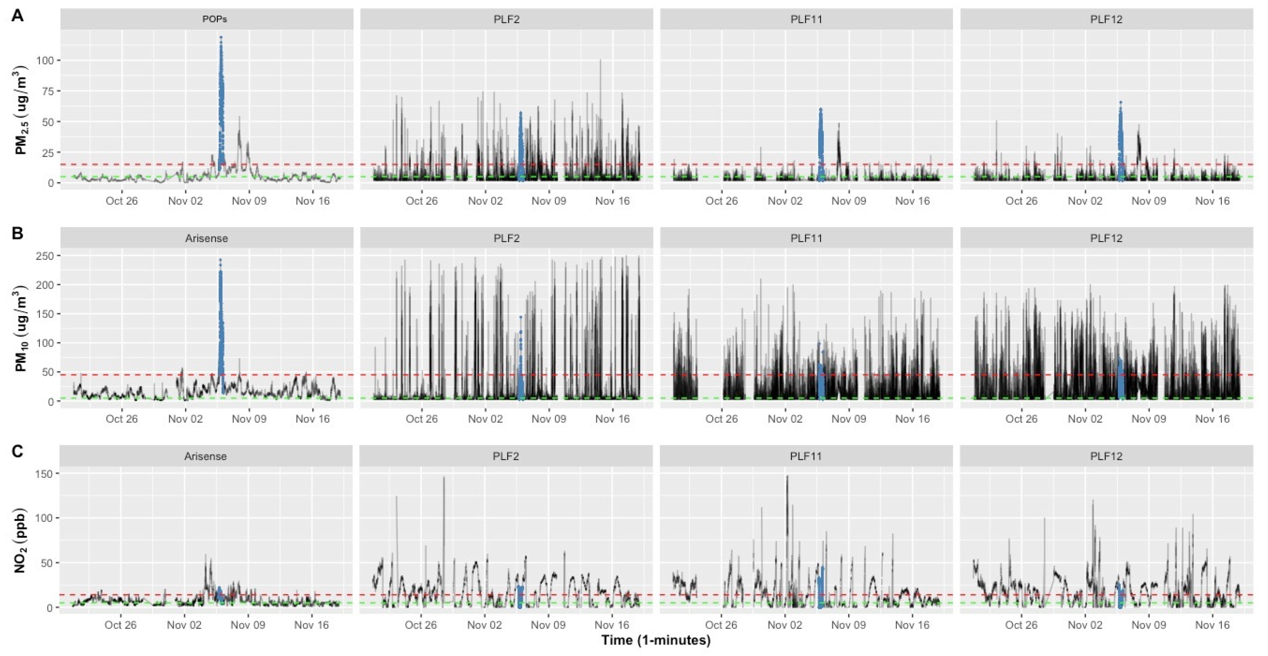
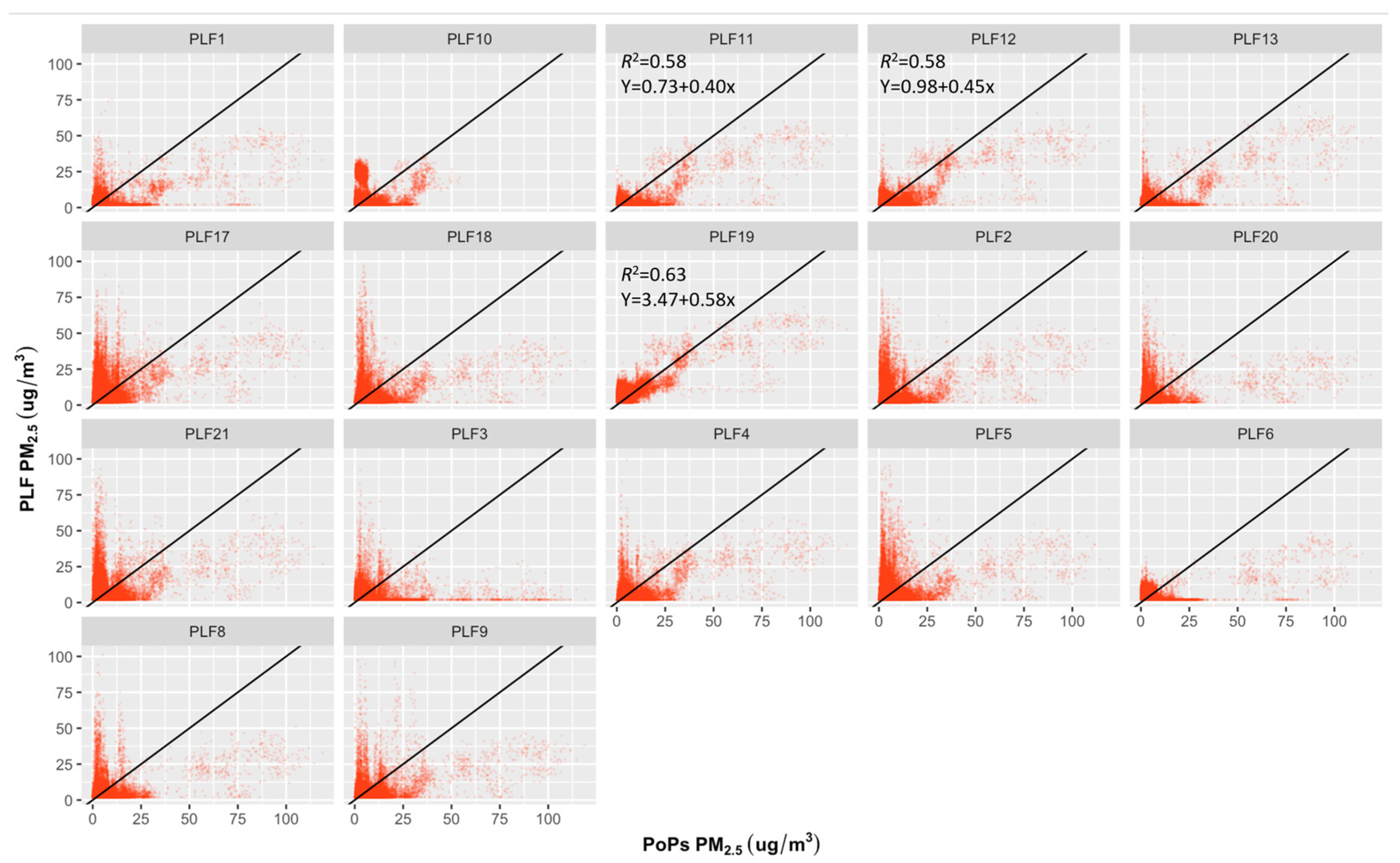
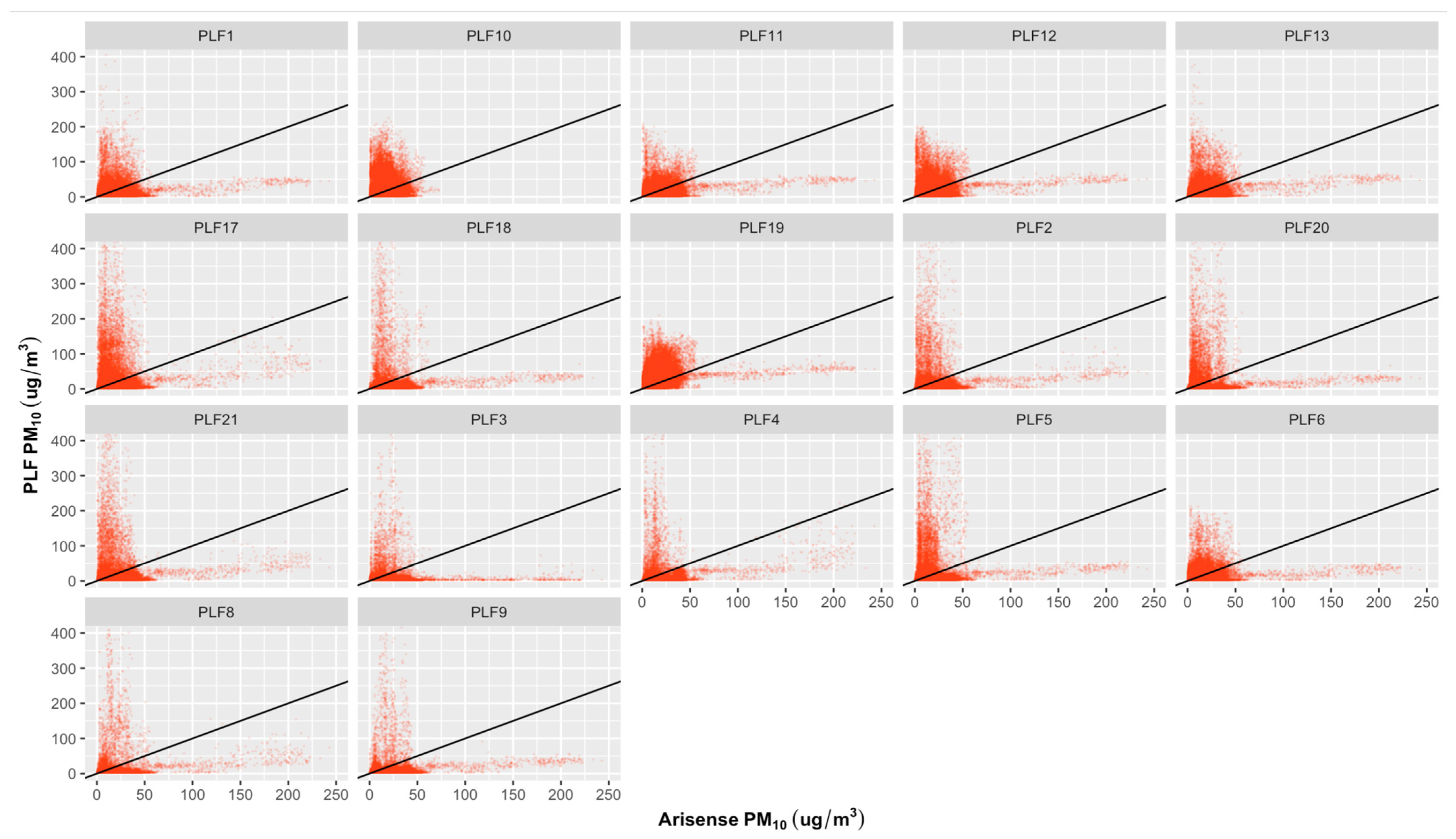
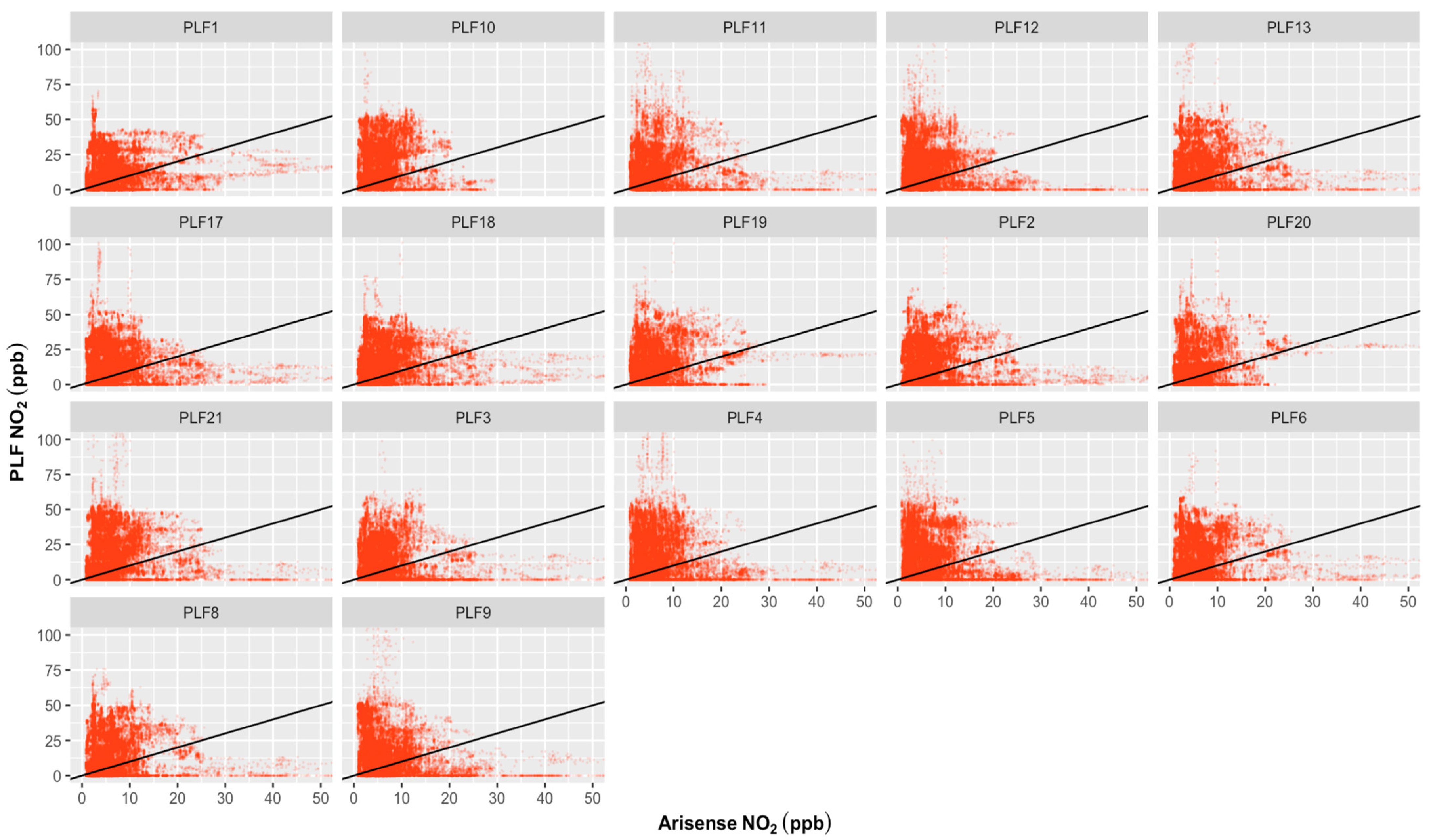
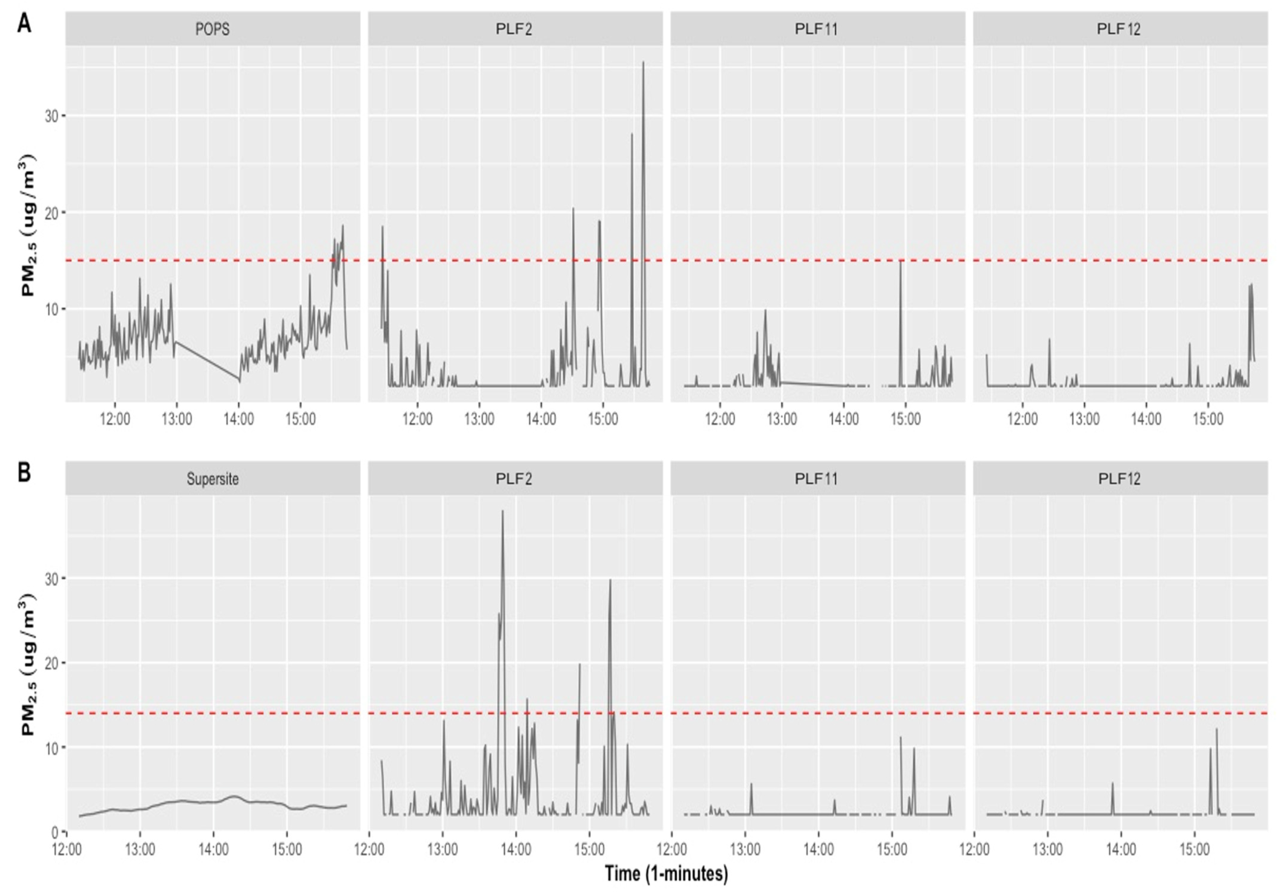
3.2. Outdoor Roadside and Supersite Intercomparison

PM_2.5 pollution levels were measured only at the roadside with the POPS instrument, and PM_2.5, PM₁₀, and NO₂ levels were measured at the outdoor Supersite. Due to the short time period of the measurements, only descriptive and correlation coefficient analyses for each site were conducted. At the time of measurements, the air quality measurements at both sites (road and Supersite locations) showed concentrations lower than the WHO 24 h mean limit value (see Figures S2 and S3). An elevated concentration of PM_2.5 was observed for periods between 3:30 p.m. and 3:41 p.m. (13 November 2020), as detected by POPS at the roadside location for PM_2.5, with the maximum level reaching 18.60 μg/m³ (see Figure 5A).

Tables S2 and S3 provide a summary of the roadside and Supersite pollutants measured by the PLFs, and reference POPS and Supersite instruments. The roadside mean concentration of PM_2.5 recorded by PLFs ranged between 2.4 and 18.54 μg/m³ (maximum of 12.54–75.18 μg/m³), with a mean concentration of 7.12 μg/m³ (maximum of 18.6 μg/m³) with measurements taken by POPS. Findings from the Supersite location showed that the mean concentration of PM_2.5, PM₁₀, and NO₂ recorded by PLFs ranged between 2.12 and 7.72 μg/m³ (maximum of 11.25–78.91 μg/m³), 8.14 and 27.59 μg/m³ (maximum of 115.41–572.93 μg/m³), and 1.8 and 23.89 ppb (maximum of 15.97–183.3 ppb), respectively, while the mean concentration was 3.05 μg/m³, 6.48 μg/m³, and 9.92 ppb (maximum of 4.13 μg/m³, 8.8 μg/m³, and 18.38 ppb) for PM_2.5, PM₁₀, and NO₂, respectively, with measurements taken by the Supersite monitors.

The measured pollutant levels obtained from the PLFs (n = 15 units) do not show a good correlation (r < 0.4) with the concentrations measured by the POPS and Supersite instruments at both locations. Exceptional results were seen with two PLFs (PLF2 and PLF17) that showed moderate correlation (0.4 < r < 0.6) when measuring PM_2.5 at the roadside location. The correlation tables for the road and Supersite locations are given in the Supplementary Material (see Tables S8 and S9). These results were obtained using short measurement periods in the outdoor environments, but monitoring devices perform less well in outdoor locations than in indoor locations. Given that our indoor results showed that data from PLFs did not correlate well with those of reference instruments and the resulting limitations and uncertainties associated with the data, collecting more measurements over a longer period of time may not have altered our conclusions regarding their worth in assessing outdoor air pollution.

Our field evaluation results show, at best, a weak correlation between the majority of the PLF devices (n = 16) and the reference instruments for all measured pollutants. Only one PLF showed a moderate correlation with the reference data. Our results are in agreement with another field evaluation reported by the South Coast AQMD [23]. Their R² for PM_2.5 measurement was between 0.02 and 0.15 for three PLF units and a Federal Equivalent Monitor GRIMM (FEM GRIMM) over an hour period, and was stronger over 24 h of observation (0.02 < R² < 0.72) compared to 5 min (0.01 < R² < 0.09) [22].

4. Conclusions

There is increasing adoption of commercial low-cost air quality monitors by health researchers and public authorities. The body of literature assessing the accuracy of these devices is continuously expanding, but little is reported on commercially available personal exposure monitors. In our study, we conducted a comprehensive assessment of the market-leading real-time air quality exposure monitor, the Plume Lab Flow2, which included events with highly variable pollution levels. Our study serves a specific purpose in highlighting the performance characteristics and limitations of these widely used low-cost sensors under real-world conditions. Their performance was evaluated by comparing their air pollutant measurements (PM_2.5, PM₁₀, and NO₂) against readings from several high-quality air pollution monitors (ARISense, POPS, and Manchester Air Quality Supersite monitoring sites) under field conditions at indoor, outdoor, and roadside locations.

Our indoor study demonstrated little or no correlation between results from different PLFs and between PLFs and reference instruments, suggesting that these instruments are of little value in assessing indoor air quality. Given that most people spend more time indoors than outdoors, it is unlikely that these PLFs would provide an accurate estimate of human exposure to indoor air pollutants; hence, their value for epidemiological studies would be limited. Our outdoor study provided some evidence that the PLFs did not provide comparable data nor respond in the same way, but this conclusion is based upon a short measurement period, which is a limitation of the present work. Longer measurement periods can generally provide a more comprehensive understanding of instrument performance, but monitoring devices perform less well in outdoor locations than in indoor locations (e.g., Rai et al. “End-user perspective of low-cost sensors for outdoor air pollution monitoring” Sci Total Env 2017; 607-608, 691-705 [34]). The available evidence suggests that these PLFs would also have little value in assessing outdoor air pollution given the poor performance of PLFs in indoor locations.

Our evidence from the indoor studies also suggests that these PLFs do not necessarily perform better at higher pollutant levels, given the high variability in response to a known high pollution event (Guy Fawkes night). It is thus currently not possible to identify any circumstance where these monitors could be used to accurately assess pollution levels (especially indoors). Rather, this study suggests the importance of assessing PLF performance against the use of reference instruments so as to assess, in particular, the accuracy of PLFs. Utilizing reference instruments and established facilities can enable the evaluation of PLF performance in a controlled and standardized manner. Another limitation arises from the use of multiple different reference instruments, which may introduce a potential bias that is challenging to quantify. Further studies should examine whether PLFs maintain their performance over extended durations to accurately represent their potential real-world applications. Accordingly, a comparison of personal monitoring devices with corresponding reference methods should be a routine quality assurance to continue developing more efficient sensors, to guarantee the reliability of the data.

References

1. Li, X.; Huang, S.; Jiao, A.; Yang, X.; Yun, J.; Wang, Y.; Xue, X.; Chu, Y.; Liu, F.; Liu, Y.; et al. Association between Ambient Fine Particulate Matter and Preterm Birth or Term Low Birth Weight: An Updated Systematic Review and Meta-Analysis. Environ. Pollut. 2017, 227, 596–605. [Google Scholar] [CrossRef]
2. Manisalidis, I.; Stavropoulou, E.; Stavropoulos, A.; Bezirtzoglou, E. Environmental and Health Impacts of Air Pollution: A Review. Front Public Health 2020, 8, 14. [Google Scholar] [CrossRef]
3. Cohen, A.J.; Brauer, M.; Burnett, R.; Anderson, H.R.; Frostad, J.; Estep, K.; Balakrishnan, K.; Brunekreef, B.; Dandona, L.; Dandona, R.; et al. Estimates and 25-Year Trends of the Global Burden of Disease Attributable to Ambient Air Pollution: An Analysis of Data from the Global Burden of Diseases Study 2015. Lancet 2017, 389, 1907–1918. [Google Scholar] [CrossRef] [PubMed]
4. Lin, X.; Luo, J.; Liao, M.; Su, Y.; Lv, M.; Li, Q.; Xiao, S.; Xiang, J. Wearable Sensor-Based Monitoring of Environmental Exposures and the Associated Health Effects: A Review. Biosensors 2022, 12, 1131. [Google Scholar] [CrossRef] [PubMed]
5. Hoek, G. Methods for Assessing Long-Term Exposures to Outdoor Air Pollutants. Curr. Environ. Health Rep. 2017, 4, 450–462. [Google Scholar] [CrossRef] [PubMed]
6. Zou, B.; Wilson, J.G.; Zhan, F.B.; Zeng, Y. Air Pollution Exposure Assessment Methods Utilized in Epidemiological Studies. J. Environ. Monit. 2009, 11, 475–490. [Google Scholar] [CrossRef] [PubMed]
7. Monn, C. Exposure Assessment of Air Pollutants: A Review on Spatial Heterogeneity and Indoor/Outdoor/Personal Exposure to Suspended Particulate Matter, Nitrogen Dioxide and Ozone. Atmos. Environ. 2001, 35, 1–32. [Google Scholar] [CrossRef]
8. Duan, N.; Mage, D.T. Combination of Direct and Indirect Approaches for Exposure Assessment. J. Expo. Anal. Environ. Epidemiol. 1997, 7, 439–470. [Google Scholar] [PubMed]
9. Watson, A.Y.; Bates, R.R.; Kennedy, D. Assessment of Human Exposure to Air Pollution: Methods, Measurements, and Models; National Academies Press (US): Cambridge, MA, USA, 1988. [Google Scholar]
10. Wu, J.; Jiang, C.; Liu, Z.; Houston, D.; Jaimes, G.; McConnell, R. Performances of Different Global Positioning System Devices for Time-Location Tracking in Air Pollution Epidemiological Studies. Environ. Health Insights 2010, 4, 93–108. [Google Scholar] [CrossRef] [PubMed]
11. Liu, M.; Barkjohn, K.K.; Norris, C.; Schauer, J.J.; Zhang, J.; Zhang, Y.; Hu, M.; Bergin, M. Using Low-Cost Sensors to Monitor Indoor, Outdoor, and Personal Ozone Concentrations in Beijing, China. Environ. Sci. Process. Impacts 2020, 22, 131–143. [Google Scholar] [CrossRef]
12. Borghi, F.; Spinazzè, A.; Rovelli, S.; Campagnolo, D.; Del Buono, L.; Cattaneo, A.; Cavallo, D.M. Miniaturized Monitors for Assessment of Exposure to Air Pollutants: A Review. Int. J. Environ. Res. Public Health 2017, 14, 909. [Google Scholar] [CrossRef]
13. Chambliss, S.E.; Pinon, C.P.R.; Messier, K.P.; LaFranchi, B.; Upperman, C.R.; Lunden, M.M.; Robinson, A.L.; Marshall, J.D.; Apte, J.S. Local- and Regional-Scale Racial and Ethnic Disparities in Air Pollution Determined by Long-Term Mobile Monitoring. Proc. Natl. Acad. Sci. USA 2021, 118, e2109249118. [Google Scholar] [CrossRef]
14. Gaskins, A.J.; Hart, J.E. The Use of Personal and Indoor Air Pollution Monitors in Reproductive Epidemiology Studies. Paediatr. Perinat. Epidemiol. 2020, 34, 513–521. [Google Scholar] [CrossRef]
15. Ong, H.; Holstius, D.; Li, Y.; Seto, E.; Wang, M. Air Pollution and Child Obesity: Assessing the Feasibility of Measuring Personal PM2.5 Exposures and Behaviours Related to BMI in Preschool-Aged Children in China. Obes. Med. 2019, 16, 100149. [Google Scholar] [CrossRef]
16. Chen, L.-W.A.; Olawepo, J.O.; Bonanno, F.; Gebreselassie, A.; Zhang, M. Schoolchildren’s Exposure to PM2.5: A Student Club–Based Air Quality Monitoring Campaign Using Low-Cost Sensors. Air Qual. Atmos. Health 2020, 13, 543–551. [Google Scholar] [CrossRef]
17. Mead, M.I.; Popoola, O.A.M.; Stewart, G.B.; Landshoff, P.; Calleja, M.; Hayes, M.; Baldovi, J.J.; McLeod, M.W.; Hodgson, T.F.; Dicks, J.; et al. The Use of Electrochemical Sensors for Monitoring Urban Air Quality in Low-Cost, High-Density Networks. Atmos. Environ. 2013, 70, 186–203. [Google Scholar] [CrossRef]
18. Cattaneo, A.; Garramone, G.; Taronna, M.; Peruzzo, C.; Cavallo, D.M. Personal Exposure to Airborne Ultrafine Particles in the Urban Area of Milan. J. Phys. Conf. Ser. 2009, 151, 012039. [Google Scholar] [CrossRef]
19. Castell, N.; Dauge, F.R.; Schneider, P.; Vogt, M.; Lerner, U.; Fishbain, B.; Broday, D.; Bartonova, A. Can Commercial Low-Cost Sensor Platforms Contribute to Air Quality Monitoring and Exposure Estimates? Environ. Int. 2017, 99, 293–302. [Google Scholar] [CrossRef] [PubMed]
20. Snyder, E.G.; Watkins, T.H.; Solomon, P.A.; Thoma, E.D.; Williams, R.W.; Hagler, G.S.W.; Shelow, D.; Hindin, D.A.; Kilaru, V.J.; Preuss, P.W. The Changing Paradigm of Air Pollution Monitoring. Environ. Sci. Technol. 2013, 47, 11369–11377. [Google Scholar] [CrossRef]
21. Morawska, L.; Thai, P.K.; Liu, X.; Asumadu-Sakyi, A.; Ayoko, G.; Bartonova, A.; Bedini, A.; Chai, F.; Christensen, B.; Dunbabin, M.; et al. Applications of Low-Cost Sensing Technologies for Air Quality Monitoring and Exposure Assessment: How Far Have They Gone? Environ. Int. 2018, 116, 286–299. [Google Scholar] [CrossRef]
22. Crnosija, N.; Levy Zamora, M.; Rule, A.M.; Payne-Sturges, D. Laboratory Chamber Evaluation of Flow Air Quality Sensor PM2.5 and PM10 Measurements. Int. J. Environ. Res. Public Health 2022, 19, 7340. [Google Scholar] [CrossRef] [PubMed]
23. South Coast. Air Quality Management District Sensors. Available online: https://www.aqmd.gov/aq-spec/sensors (accessed on 18 March 2023).
24. Leung, D.Y.C. Outdoor-Indoor Air Pollution in Urban Environment: Challenges and Opportunity. Front. Environ. Sci. 2015, 2, 69. [Google Scholar] [CrossRef]
25. Cross, E.S.; Williams, L.R.; Lewis, D.K.; Magoon, G.R.; Onasch, T.B.; Kaminsky, M.L.; Worsnop, D.R.; Jayne, J.T. Use of Electrochemical Sensors for Measurement of Air Pollution: Correcting Interference Response and Validating Measurements. Atmos. Meas. Tech. 2017, 10, 3575–3588. [Google Scholar] [CrossRef]
26. Manchester Air Quality Super Site at the Firs Environmental Research Station, Fallowfield Campus. Available online: http://www.cas.manchester.ac.uk/restools/firs/ (accessed on 3 October 2023).
27. Flow 2 Pocket-Sized Pollution Revolution. Available online: https://plumelabs.com/en/flow/ (accessed on 3 October 2023).
28. Gao, R.S.; Telg, H.; McLaughlin, R.J.; Ciciora, S.J.; Watts, L.A.; Richardson, M.S.; Schwarz, J.P.; Perring, A.E.; Thornberry, T.D.; Rollins, A.W.; et al. A Light-Weight, High-Sensitivity Particle Spectrometer for PM2.5 Aerosol Measurements. Aerosol Sci. Technol. 2016, 50, 88–99. [Google Scholar] [CrossRef]
29. Barker, P.A.; Allen, G.; Flynn, M.; Riddick, S.; Pitt, J.R. Measurement of Recreational N2O Emisions from an Urban Environment in Manchester, UK. Urban Clim. 2022, 46, 101282. [Google Scholar] [CrossRef]
30. Bittner, A.S.; Cross, E.S.; Hagan, D.H.; Malings, C.; Lipsky, E.; Grieshop, A.P. Performance characterization of low-cost air quality sensors for off-grid deployment in rural Malawi. Atmos. Meas. Tech. 2022, 15, 3353–3376. [Google Scholar] [CrossRef]
31. Dales, R.; Liu, L.; Wheeler, A.J.; Gilbert, N.L. Quality of Indoor Residential Air and Health. CMAJ 2008, 179, 147–152. [Google Scholar] [CrossRef] [PubMed]
32. The R Project for Statistical Computing. Available online: https://www.r-project.org/ (accessed on 3 October 2023).
33. Diez, S.; Lacy, S.E.; Bannan, T.J.; Flynn, M.; Gardiner, T.; Harrison, D.; Marsden, N.; Martin, N.A.; Read, K.; Edwards, P.M. Air pollution measurement errors: Is your data fit for purpose? Atmos. Meas. Tech. 2022, 15, 4091–4105. [Google Scholar] [CrossRef]
34. Rai, A.C.; Kumar, P.; Pilla, F.; Skouloudis, A.N.; Di Sabatino, S.; Ratti, C.; Yasar, A.; Rickerby, D. End-user perspective of low-cost sensors for outdoor air pollution monitoring. Sci. Total Environ. 2017, 607–608, 691–705. [Google Scholar] [CrossRef]
Figure 1. Time series of POPS and ARISense devices (reference) and three PLF tools for (A) PM2.5, (B) PM10, and (C) NO2 concentrations carried out over a three-week period at the indoor monitoring site. To provide a reference point, the red dashed line represents the WHO limited value (45 µg/m3 for 24 h mean PM10, 15 µg/m3 for 24 h mean PM2.5, and 25 µg/m3 (13.3 ppb) for 24 h mean NO2). The green dashed line represents the WHO limit value (15 µg/m3 for annual mean PM10), (5 µg/m3 for annual mean PM2.5, and 10 µg/m3 (5.314 ppb) for annual mean NO2). The black line represents the concentration levels. The Guy Fawkes event is colored with a blue line. The PLF2 was chosen because it best captures the characteristics of the other plumes. PLF11 and PLF12 were selected as the best-performing sensors.
Atmosphere 15 00315 g001
Figure 2. Regression plots for PLFs and POPS reference device for the 1 min PM2.5 concentrations carried out over a three-week period at the indoor monitoring location. X-axis represents POPs reference instrument; Y-axis represents PLFs tools; ----: Black line represents the 1:1 line. For those associations between the measured PM2.5 concentrations from PLFs and POPS with an R2 > 0.5, the equation for linear regression is included.
Atmosphere 15 00315 g002
Figure 3. Regression plots for PLFs and ARISense reference device for the 1 min PM10 concentrations carried out over a three-week period at the indoor monitoring location. X-axis represents ARISense reference instrument; Y-axis represents PLFs tools; ----: Black line represents the 1:1 line. No linear associations between the measured PM10 concentrations from PLFs and ARISense were observed. The density plot for this figure can be seen in Figure S5.
Atmosphere 15 00315 g003
Figure 4. Regression plots for PLFs and ARISense reference device for the 1 min NO2 concentrations carried out over a month at the indoor monitoring location. X-axis represents ARISense reference instrument; Y-axis represent PLFs tools; ----: Black line represents the 1:1 line. No linear associations between the measured NO2 concentrations from PLFs and ARISense were observed. The density plot for this figure can be seen in Figure S6.
Atmosphere 15 00315 g004
Figure 5. Time series of POPS and Supersite monitors (reference) and three PLF tools for PM2.5, 1 min concentrations carried out for over three hours at the (A) roadside and (B) Manchester Air Quality Supersite. To provide a reference point, the red dashed line represents the WHO limited value (15 µg/m3 for 24 h mean PM2.5).
Atmosphere 15 00315 g005