3.1. General Description of Visibility, Meteorology and Air Pollution
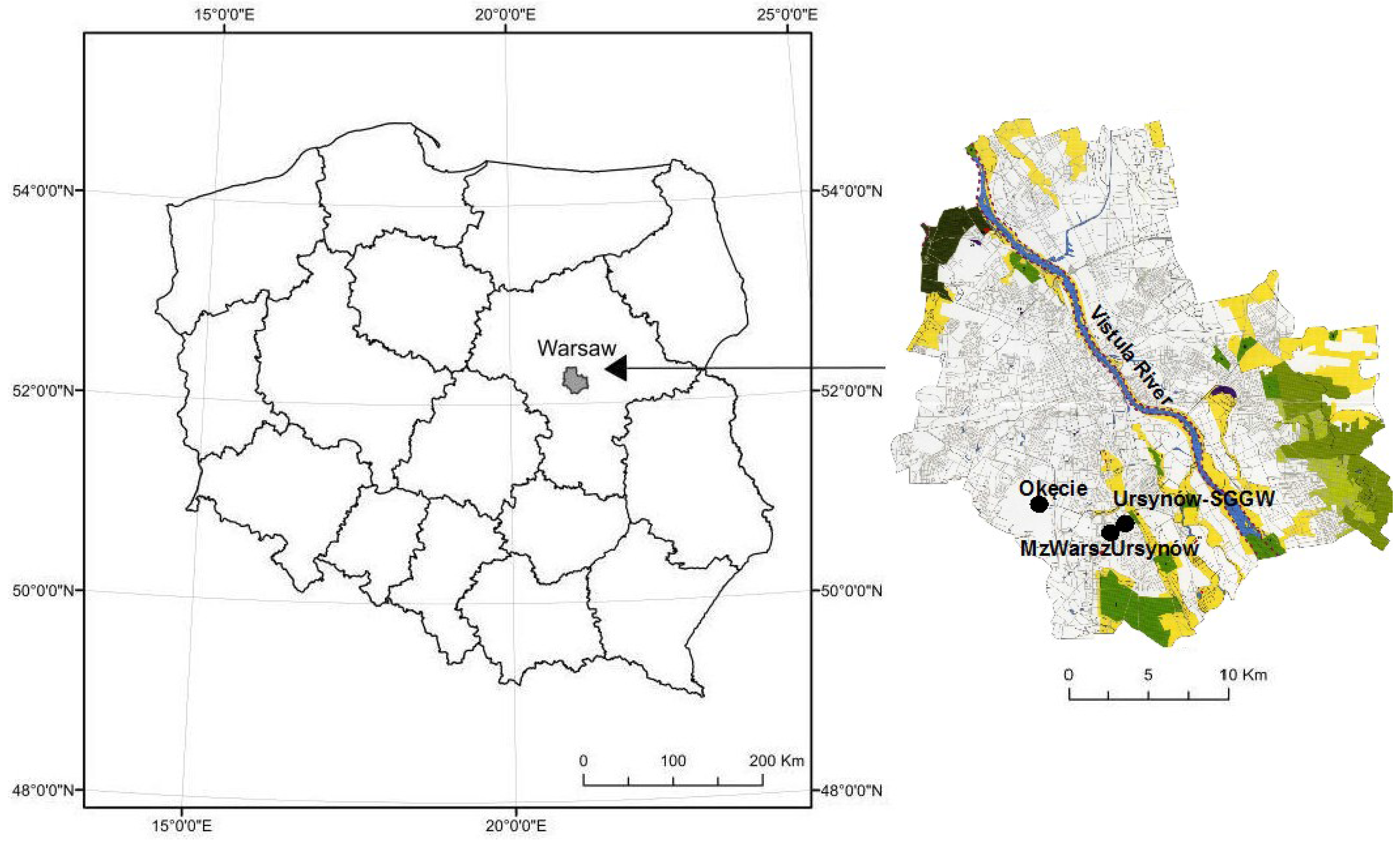
The yearly course of the air temperature (average in the period 2004–2013) was typical for the temperate and transitional climate in Poland. July was the warmest month (mean air temperature = 20.5 °C). January was the coldest month (mean air temperature = −2.1 °C). The lowest wind speed values were measured in August and September (approx. 2.1 m/s), whereas the highest ones were observed in March (3.1 m/s)—
Figure 2.
Figure 2.
Monthly variations of meteorological parameters over Warsaw in 2004–2013.
Figure 2.
Monthly variations of meteorological parameters over Warsaw in 2004–2013.
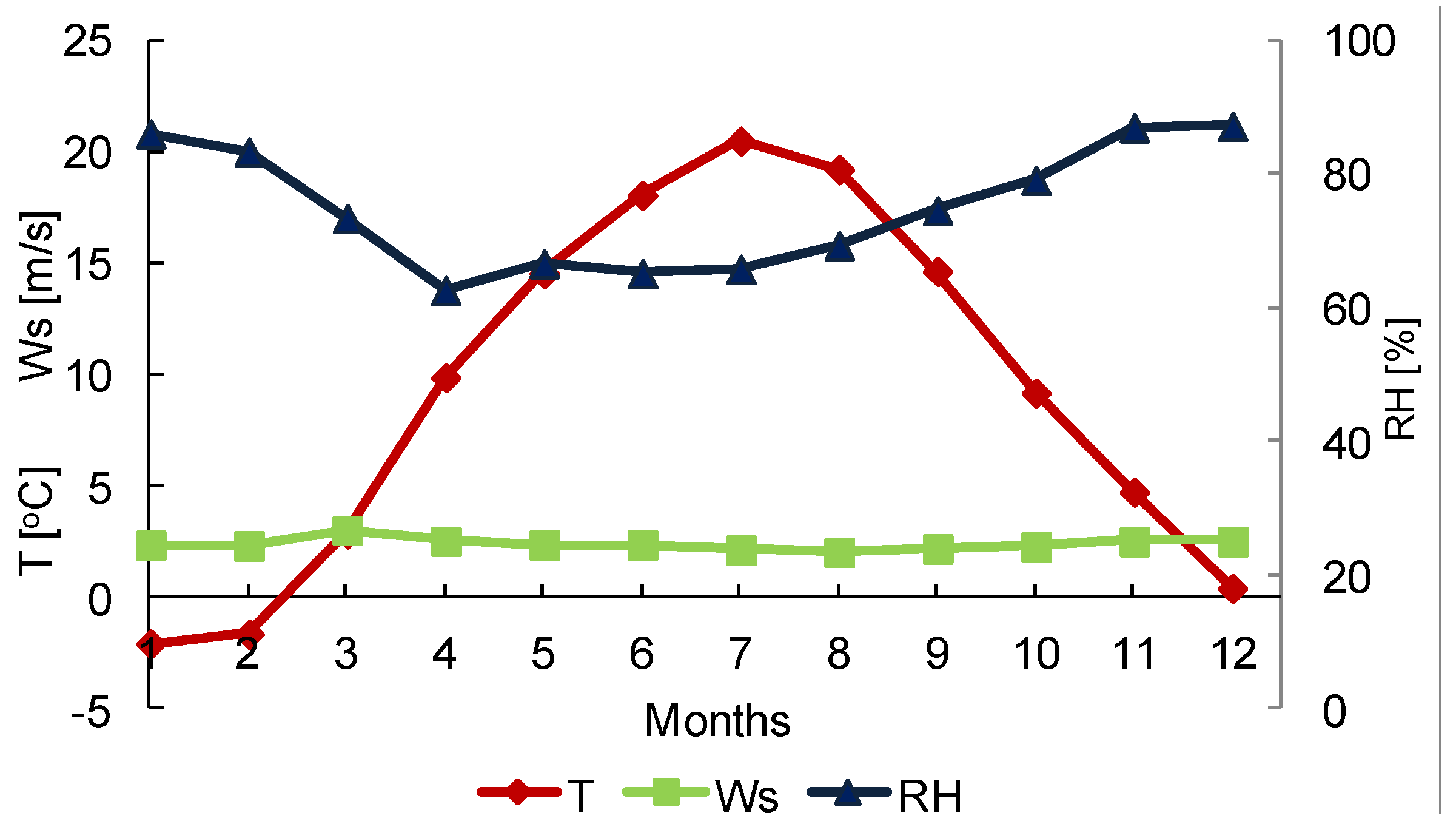
Figure 3 presents the diurnal patterns of visibility for the period 2004–2013. Visibility shows an obvious diurnal variation in each season of the year. In spring (March, April, May) and summer (June, July, August), a valley appears in early morning, from 04:00 to 06:00, while in autumn (September, October, November) and spring it is observed slightly later, between 06:00 and 07:00. The peak appears generally in the afternoon, from 13:00 to 15:00, except for winter (December, January, February), for which the peak is slightly later, at about 18:00. Visibility shows stronger diurnal cycles in summer and autumn, while it exhibits a much weaker variation in winter. Apart from this, the diurnal patterns during different seasons are desynchronized, which is attributed to the difference in weather patterns and stability of atmospheric boundary layer. The diurnal variation of visibility, characteristic for the city of Warsaw, is similar to that over several cities in China, however, hourly visibility values are found to be three times higher than those recorded in the Chinese cities [
19].
Figure 3.
Diurnal variations of visibility over Warsaw for winter (December, January, February), spring (March, April, May), summer (June, July, August) and autumn (September, October, November) in 2004–2013.
Figure 3.
Diurnal variations of visibility over Warsaw for winter (December, January, February), spring (March, April, May), summer (June, July, August) and autumn (September, October, November) in 2004–2013.
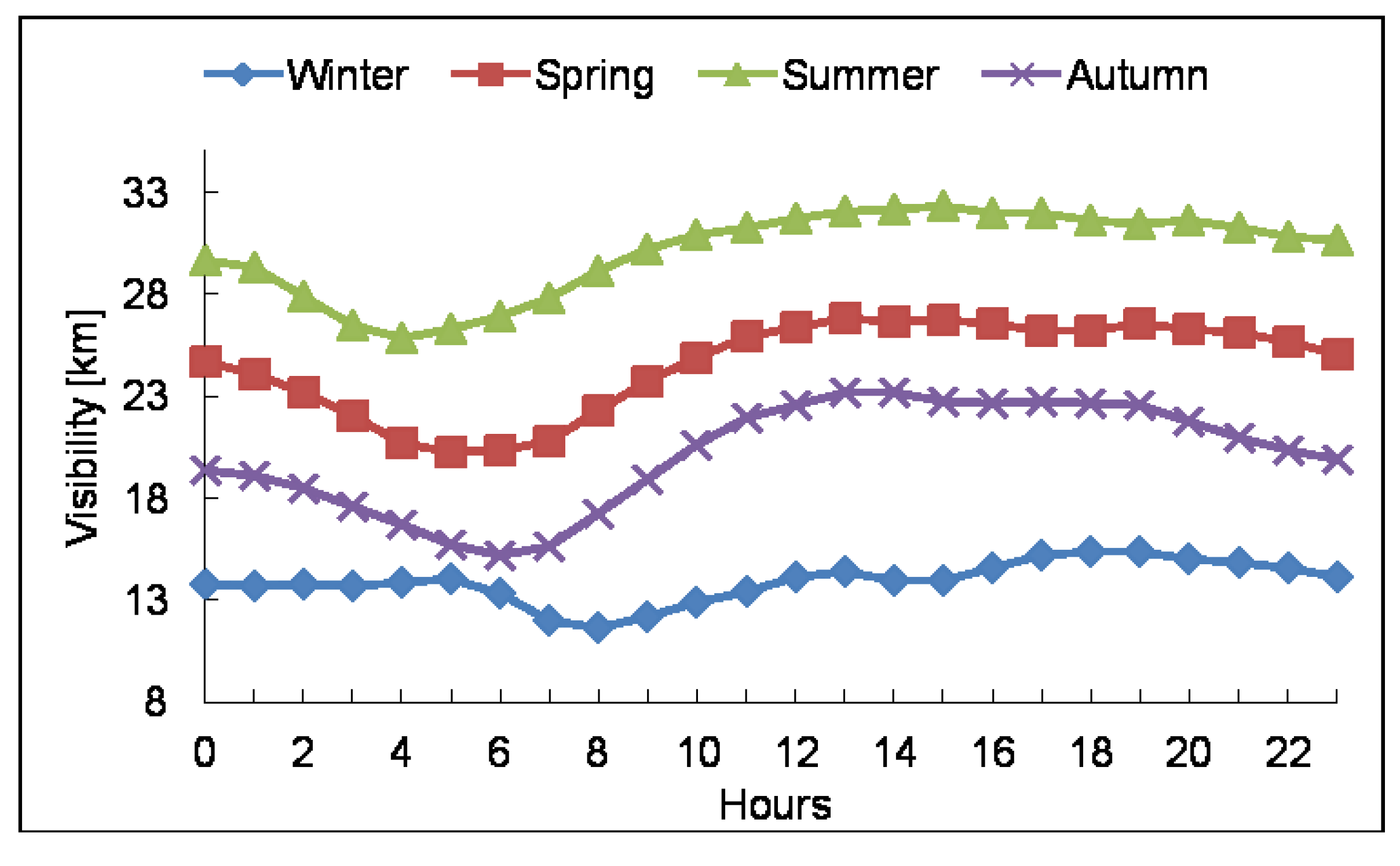
For the whole research period (2004–2013) monthly visibility was in a wide range of 6.7–34.1 km (
Figure 4). Within the researched period, noticeable seasonal changes in visibility were found. Visibility was generally higher in summer and lower in late autumn and winter. The average seasonal visibilities were 24.5, 30.1, 20.1, and 13.9 km in spring, summer, autumn, and winter, respectively (
Figure 4).
Figure 4.
Descriptive statistics of monthly and seasonal visibility over Warsaw in 2004–2013.
Figure 4.
Descriptive statistics of monthly and seasonal visibility over Warsaw in 2004–2013.
Monthly visibility in Warsaw exhibited, in general, a considerable winter period variation (January–March, October–November) from 2004–2013. The summer period was characterized by much lower variation.
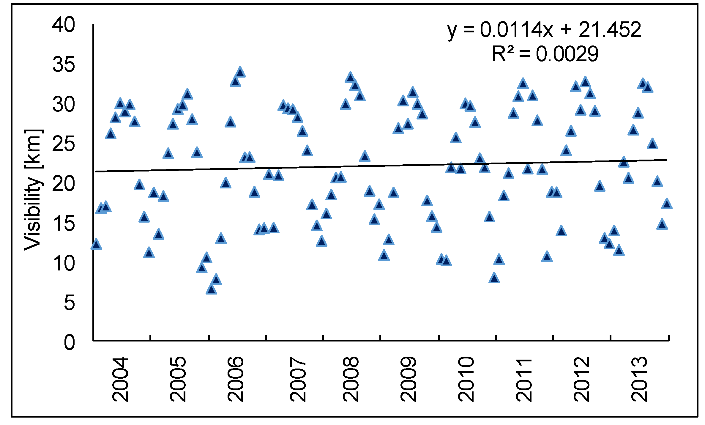
The mean yearly visibilities were in the range of 19.8–23.7 km (
Figure 5). This proves that it did not show significant variability year by year. However, monthly values exhibit an increasing trend throughout the research period, but are statistically insignificant;
p < 0.05 (
Figure 6). Average visibility for the whole period 2004–2013 was equal to 22.1 km and is from 5.3 km to over 13.1 km higher than the one over large, highly urbanized cities of China [
1,
19].
Figure 5.
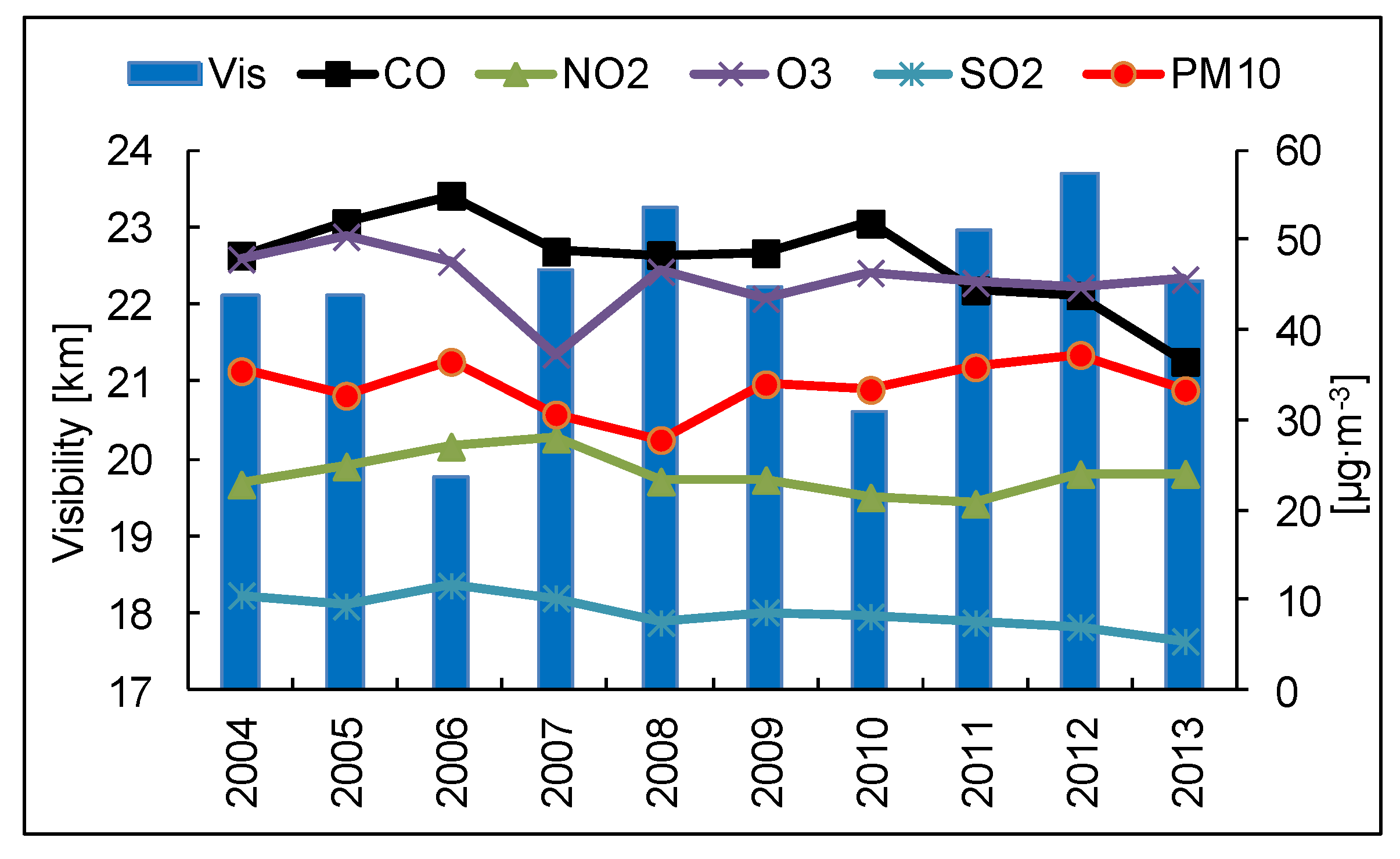
Yearly variations of visibility and ambient concentrations of NO2, O3, SO2, PM10 and CO (divided by 10 in the figure) over Warsaw in 2004–2013.
Figure 5.
Yearly variations of visibility and ambient concentrations of NO2, O3, SO2, PM10 and CO (divided by 10 in the figure) over Warsaw in 2004–2013.
Figure 6.
Visibility time series of monthly mean and its’ linear regression trend over Warsaw in 2004–2013.
Figure 6.
Visibility time series of monthly mean and its’ linear regression trend over Warsaw in 2004–2013.
From 2004–2013 yearly air pollutants concentration didn’t show much variation, alike visibility. In the analysed years, the mean yearly concentrations of NO
2 were 21.4–28.0 μg·m
−3, which made 53.6%–70% of the permissible value (40 μg·m
−3)—
Figure 5. The mean yearly concentrations of SO
2 were 5.5–11.5 μg·m
−3 (the permissible value; 20 µg·m
−3), and the mean yearly concentrations of CO were 365.7–549.5 μg·m
−3. The mean yearly concentrations of PM
10 did not exceed the permissible value as well (40 µg·m
−3) and were in the range of 28.0–37.2 µg·m
−3. The only pollutant, that, according to the Polish applicable laws, exceeded the permissible limit, was the ozone O
3. The mean yearly concentrations of O
3 were 43.5–50.4 µg·m
−3. The permissible level of the 8-h O
3 concentration is 120 µg·m
−3 and can be exceeded about 25 days in each year. The biggest number of days with the exceeded value was observed in 2005. In the research area, there was no steady trend in the changes for O
3, which is a secondary pollutant. The changes in its concentration mainly resulted from the changes in the weather conditions (insolation intensity, air temperature) and the participation of the O
3 precursors (e.g., nitrogen oxides, hydrocarbons and other pollutants participation in the O
3 formation) in the atmospheric air [
30,
39].
Since the visibility is strongly affected by air pollutants [
1,
40,
41], the presence of its’ weaker variation over Warsaw from 2004–2013 is found. In Poland, considerable changes in air pollution were observed from 1980–2000 [
42]. In that period, political and economical transformation was related with a sudden decrease of industrial emission due to large factories closure and limited production in remaining ones [
43,
44]. On the other hand, such transformation contributed to the knowledge on negative consequences of air pollution, and for this reason in 1980s industrial emissions were largely restricted in Poland. Unfortunately, no reliable air pollution measurements were then performed within the research area.
Figure 7.
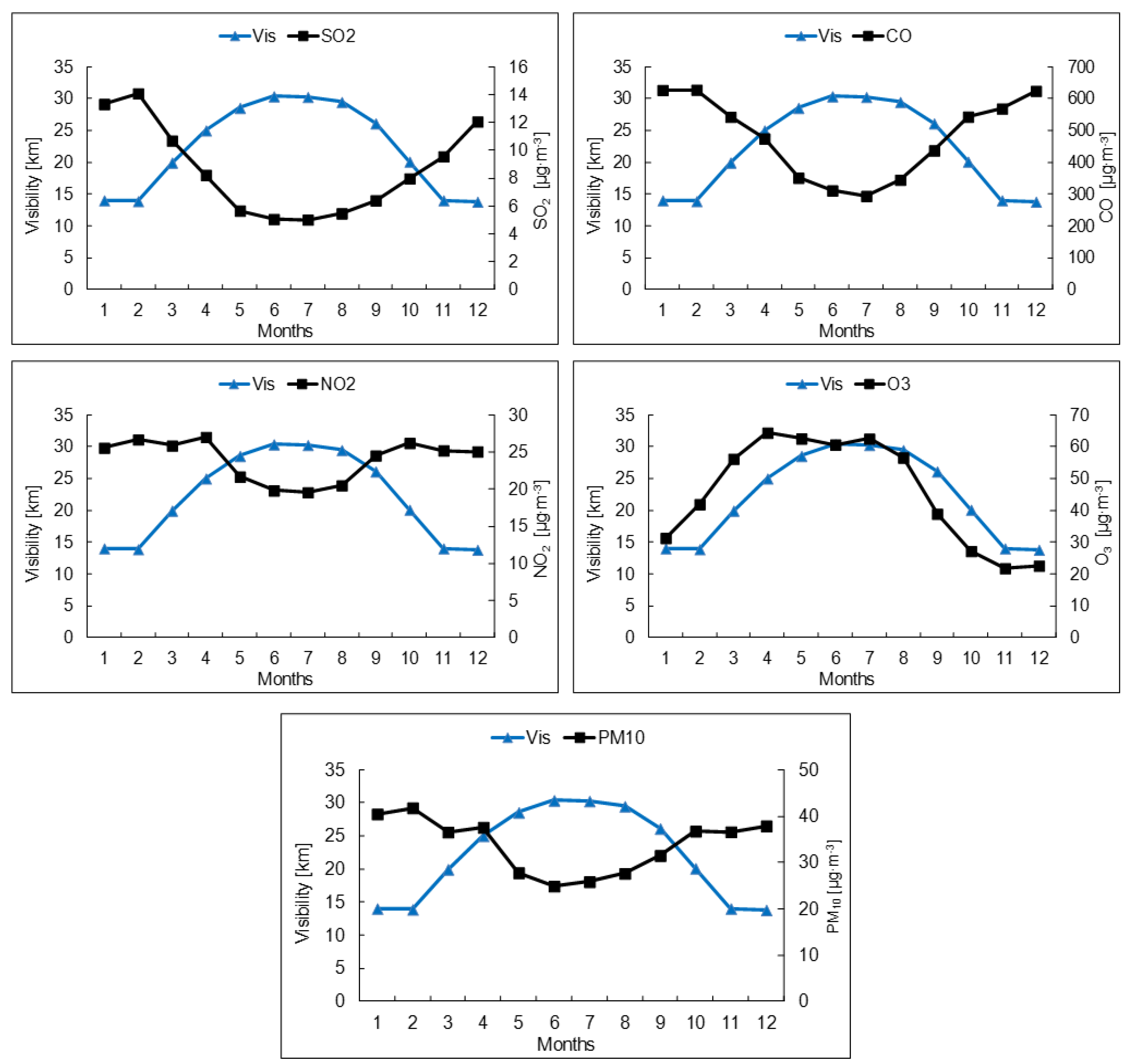
Monthly variations of visibility and ambient concentrations of air pollutants over Warsaw in 2004–2013.
Figure 7.
Monthly variations of visibility and ambient concentrations of air pollutants over Warsaw in 2004–2013.
Monthly visibilities and monthly ambient concentrations of air pollutants (averages for the whole period 2004–2013) are shown in
Figure 7. Comparing the maximum and minimum values for the monthly concentrations shows that O
3, CO and SO
2 have the largest variability; while much lower variability was shown by PM
10 and NO
2. Visibility values were inversely proportional to all analysed pollutants, except for O
3. Ambient concentrations of PM
10, SO
2, NO
2 and CO tend to be strongly affected by the emission from fuel combustion for heating purposes [
31,
45]. It is obvious that their concentration is higher in winter months, while the visibility becomes lower (
Figure 7). Except for the higher winter emission in Poland, the increase of air pollution is also attributed to meteorological conditions (lowering of air mixing layer, stagnant air) that deteriorate ventilation and ability of self-cleaning [
46]. The fact that concentrations of CO, NO
2 and SO
2 are higher in the cold season (
Figure 7) is attributed to increased emissions—however, the atmospheric lifetime of these compounds is also generally longer in the winter and this is likely to explain some of the increase as well.
The mean NO
2 concentration was slightly higher in the cold season than in the warm one. Such a situation was related to the low variation of the yearly NO
2 emission. Typically, the data indicated two daily peaks in the ambient concentrations of both NO
x forms (NO and NO
2), which pointed to the traffic-related pollution [
30,
39]. Emission from the traffic contributes also to ambient concentrations of volatile organic compounds (VOCs). VOCs and NO react with O
3 giving a loss of O
3 near to pollution sources. On the other hand, higher O
3 in summer is probably because of higher solar insolation, and visibility is lower because of the lack of cold season emissions and boundary layer effects. For those reasons, the course of monthly ozone concentrations is different from NO
2 and other pollutants, and resembles the course of visibility.
3.3. Weekend/Weekday Differences in Visibility and Air Pollution
When referring to the visibility and air quality studies, there is a phenomenon known as the
weekend effect, Studies on this phenomenon can help to better understand the emission characteristics of air pollutants in urban areas and the weekend effect has been reported in America since the 1970s [
47,
48]. Contemporary research is especially focusing on visibility variations and the effect of air quality on visibility on weekdays compared with weekend days. In order to investigate potential weekend effect over Warsaw, mean weekend and weekday levels of visibility as well as air pollutants were calculated and subjected to Fisher–Snedecore test. Visibilities on weekends were slightly better than on weekdays, and the differences were statistically significant. Mean hourly visibility was equal to 22.61 ± 12.57 km at weekends and slightly over 22.02 ± 12.71 on weekdays (
Table 2). For PM
10, slightly higher and statistically significant weekday concentrations were observed, as well as for SO
2, which was slightly lower during weekends. We also found CO concentrations to become lower on weekends (statistically significant differences) and, moreover, mean weekend and weekday NO
2 concentrations over Warsaw showed statistically significant differences, with NO
2 concentration higher on weekdays. This is probably due to less vehicular emission on weekends.
All concentrations of airborne pollutants were higher during weekdays, (statistically significant differences), except ozone. O
3 concentration was higher at weekends even though the O
3 pollutant precursor concentrations (such as NO
x and volatile organic compounds) are lower on weekends [
47,
48]. The weekend effect in the O
3 concentrations is the most likely to be attributable to decreased O
3 destruction by NO
x, as there are lower emissions from its’ main source—communication and vehicular transportation [
48,
49]. The result of this study, concerning lower concentrations of airborne pollutants on weekends, excluding ozone, is similar to that obtained by Tsai [
17].
Table 2.
Visibility and air pollutant concentrations calculated as arithmetic means on the basis of the hourly values from 2004–2013 for two different periods—weekends and week days.
Table 2.
Visibility and air pollutant concentrations calculated as arithmetic means on the basis of the hourly values from 2004–2013 for two different periods—weekends and week days.
| | Vis | PM10 (μg·m−3) | SO2 (μg·m−3) | CO (μg·m−3) | NO2 (μg·m−3) | O3 (μg·m−3) |
|---|
| Weekend | 22.61 ± 12.57 | 32.03 ± 24.20 | 8.08 ± 6.95 | 456.45 ± 327.25 | 20.20 ± 15.74 | 48.94 ± 29.46 |
| | (n = 25,044) | (n = 23,652) | (n = 24,485) | (n = 23,782) | (n = 24,585) | (n = 24,444) |
| Weekday | 22.02 ± 12.71 | 34.66 ± 25.38 | 8.75 ± 8.15 | 485.49 ± 340.51 | 25.50 ± 17.60 | 44.51 ± 29.94 |
| | (n = 62,590) | (n = 59,364) | (n = 60,931) | (n = 59,495) | (n = 61,400) | (n = 60,704) |
| Fisher test | 62,590 | 59,364 | 60,931 | 59,495 | 61,400 | 60,704 |
| p-value | 0.0000 | 0.0000 | 0.0000 | 0.0000 | 0.0000 | 0.0000 |
3.4. Correlations between Pollutants, Meteorological Variables and Visibility
Total correlations found between the results of the visibility measurements and other measurements (mean hourly values) in the whole research period are shown in
Table 3. The visibility measurement results were negatively correlated with CO, PM
10, SO
2 and NO
2. Therefore, the increase in CO and SO
2 concentrations corresponds with visibility decrease, and PM
10 and NO
2 are those species, that can directly contribute to visual range limitations.
Table 3.
Correlation matrix for total parameters measured for the entire period of 2004–2013 (correlations calculated for hourly values) and arithmetic means and standard deviations of the hourly value sets for the measured parameters.
Table 3.
Correlation matrix for total parameters measured for the entire period of 2004–2013 (correlations calculated for hourly values) and arithmetic means and standard deviations of the hourly value sets for the measured parameters.
| | A | SD | PM10 | SO2 | CO | NO2 | O3 | T | Ws | RH | Rad | P |
|---|
| Vis (km) | 22.19 | 12.67 | −0.33 | −0.27 | −0.37 | −0.21 | 0.47 | 0.52 | 0.14 | −0.60 | 0.37 | −0.10 |
| PM10 (μg·m−3) | 33.91 | 25.07 | 1.00 | 0.37 | 0.66 | 0.56 | −0.26 | −0.23 | −0.25 | 0.05 | −0.13 | −0.04 |
| SO2 (μg·m−3) | 8.56 | 7.83 | | 1.00 | 0.34 | 0.25 | −0.15 | −0.38 | −0.10 | 0.10 | −0.07 | −0.03 |
| CO (μg·m−3) | 477.20 | 337.03 | | | 1.00 | 0.62 | −0.41 | −0.38 | −0.28 | 0.21 | −0.25 | −0.03 |
| NO2 (μg·m−3) | 23.98 | 17.26 | | | | 1.00 | −0.52 | −0.19 | −0.36 | 0.15 | −0.31 | −0.03 |
| O3 (μg·m−3) | 45.78 | 29.87 | | | | | 1.00 | 0.47 | 0.22 | −0.71 | 0.56 | 0.02 |
| T (°C) | 9.33 | 9.33 | | | | | | 1.00 | 0.03 | −0.52 | 0.48 | 0.05 |
| Ws (m/s) | 2.42 | 1.68 | | | | | | | 1.00 | −0.08 | 0.16 | 0.04 |
| RH (%) | 74.97 | 18.82 | | | | | | | | 1.00 | −0.58 | 0.06 |
| Rad (W/m2) | 117.77 | 200.98 | | | | | | | | | 1.00 | −0.03 |
| P (mm) | 0.07 | 0.52 | | | | | | | | | | 1.00 |
Visibility was positively correlated with the O
3 concentrations. The atmospheric O
3 is a secondary air pollutant formed in photochemical reactions. Hence, summer is the period of the most intense O
3 formation. It resulted from the high insolation intensity during this season. The observed correlation was caused by the fact that both parameters (visibility and O
3 concentrations) increased and decreased in the same periods (
Figure 7).
In addition to their impact on visibility via changing the concentration of pollutants, meteorological variables can affect the visibility more directly - as humidity increases, hygroscopic aerosols increase in size and thus the scattering of light by them increases. At some point, aerosols activate and become fog [
50,
51]. This transition is very complex and has a very large impact on visibility [
50,
51].
Hourly visibility exhibited low, negative correlation with precipitation (
Table 3). Generally, the precipitation lowered the air pollutant concentrations through the precipitation scavenging. Thereby, visibility increased [
52]. However, the air purification effect and related visibility improvement appears with a delay after rainy days. During heavy precipitation visibility will be reduced. However, after the precipitation has stopped, the aerosols concentration are likely to be lower, thus giving two opposite impacts with a visibility increase following rain. In fact, the visibility reduction is more likely caused by the scattering of light by the hydrometeors. There is a negative correlation between precipitation and the primary pollutants, but this is weak and may relate to improved boundary layer ventilation when there is precipitation rather than scavenging. This is suggested by the fact that the relatively insoluble CO and NO
2 have a negative correlation with precipitation, which is the same size as that of the more soluble SO
2.
Visibility was positively correlated with the three remaining meteorological parameters, air temperature, insolation intensity, and wind speed. Most likely under clear sky conditions, the temperatures increase, the relative humidity falls and so the aerosols shrink, thus increasing the visibility.
3.5. Principal Component Analysis (PCA)
PCA served to extract four principal components (new variables: PC1, PC2, PC3 and PC4) with eigenvalues >1.0, which accounted for 73% of the total variance (
Table 4). PC1, PC2, PC3 and PC4 can be interpreted as major factors that control visibility [
1,
6,
17,
40]. Visibility (Vis), O
3 concentration (O
3), NO
2 concentration (NO
2), CO concentration (CO), air temperature (T), relative air humidity (RH), PM
10 concentration (PM
10) and insolation intensity (Rad) were most strongly correlated with PC1. Knowing the research area and the influence of various emission sources in this region, it can be assumed that PC1 could be related to fuel combustion for heating (mainly hard coal, wood/biomass and heating/crude oil) [
31,
44]. The emission increased over the year along with the T drop and Rad decrease. At the same time, the pollutant concentrations (
i.e., PM
10, NO
2, CO, or SO
2) in the air increased. Simultaneously, the photochemical pollutant concentrations (represented by O
3) decreased. Visibility was reduced in periods of high air pollution, related with heating (opposite signs for Vis/PC1 correlation and PM
10, NO
2, CO, SO
2/PC1 correlation).
The PCA performed only for the cold season data (
Table 5) confirmed the same correlations between PC1 and the air pollution with NO
2, SO
2 and CO, and the inverse (opposite signs) correlation between PC1 and visibility, O
3 concentration, air temperature and insolation. For the warm season, the PCA revealed a very strong correlation between PC1 and NO
2 and an inverse strong correlation (opposite signs) between PC1 and visibility, O
3 concentration and insolation. Most likely, in those periods when there is less pollution from heating, and temperature rises, air pollution is mainly shaped by traffic emissions [
31]. Then, the increase of NO
2 is observed, which reacts with O
3 and in consequence the concentration of O
3 in the air decreases. The reaction intensity becomes higher when the insolation intensity is stronger (O
3 concentrations and insolation were correlated with PC1 in the same way). Under such conditions, visibility may be improved (contrary signs of Vis/PC1 and NO
2/PC1). Nonetheless, it is not possible to discuss the cause-and-effect correlation between the traffic emission (and the related photochemical reactions) and the visibility increase or decrease. Most probably, visibility increased because the air pollution with PM was lower and the temperature and insolation were higher in summer.
Table 4.
Correlations between the principal components (PC1, PC2, PC3, PC4) and measured parameter values. The PCA was performed for the hourly data collected in 2004–2013.
Table 4.
Correlations between the principal components (PC1, PC2, PC3, PC4) and measured parameter values. The PCA was performed for the hourly data collected in 2004–2013.
| Component | PC1 | PC2 | PC3 | PC4 |
|---|
| Vis | 0.7 | 0.3 | 0.2 | 0.2 |
| PM10 | −0.6 | 0.6 | −0.1 | −0.1 |
| SO2 | −0.4 | 0.3 | −0.6 | 0.0 |
| CO | −0.7 | 0.5 | 0.0 | −0.1 |
| NO2 | −0.7 | 0.5 | 0.3 | 0.0 |
| O3 | 0.8 | 0.3 | −0.3 | −0.1 |
| T | 0.7 | 0.3 | 0.4 | −0.2 |
| Ws | 0.4 | −0.3 | −0.5 | 0.0 |
| RH | −0.7 | −0.6 | 0.1 | 0.0 |
| Rad | 0.6 | 0.4 | −0.3 | −0.1 |
| P | 0.0 | −0.2 | 0.0 | −0.9 |
| eigenvalue | 4.06 | 1.79 | 1.12 | 1.02 |
| % total variance | 37 | 16 | 10 | 9 |
| Cumul. % variance | 37 | 53 | 63 | 73 |
Table 5.
Correlations between the principal components (PC1, PC2, PC3) and measured parameter values. The PCA was performed for the hourly data collected in 2004–2013, separately for the cold (January–March and October–December) and warm (April–September) seasons.
Table 5.
Correlations between the principal components (PC1, PC2, PC3) and measured parameter values. The PCA was performed for the hourly data collected in 2004–2013, separately for the cold (January–March and October–December) and warm (April–September) seasons.
| Component | Season | PC1 | PC2 | PC3 | Season | PC1 | PC2 | PC3 |
|---|
| Vis. | cold | −0.7 | 0.3 | −0.1 | warm | −0.5 | −0.3 | −0.5 |
| PM10 | 0.7 | 0.5 | −0.1 | 0.4 | −0.7 | 0.2 |
| SO2 | 0.4 | 0.4 | 0.4 | 0.1 | −0.4 | 0.5 |
| CO | 0.8 | 0.4 | −0.1 | 0.6 | −0.5 | 0.1 |
| NO2 | 0.7 | 0.3 | −0.3 | 0.7 | −0.5 | −0.1 |
| O3 | −0.7 | 0.4 | 0.4 | −0.8 | −0.2 | 0.2 |
| T | −0.4 | −0.1 | −0.8 | −0.6 | −0.4 | 0.0 |
| Ws | −0.6 | 0.0 | 0.0 | −0.4 | 0.3 | 0.4 |
| RH | 0.5 | −0.8 | 0.1 | 0.7 | 0.6 | 0.0 |
| Rad. | −0.4 | 0.6 | −0.1 | −0.7 | −0.2 | 0.2 |
| P | 0.0 | −0.3 | 0.0 | 0.0 | 0.2 | 0.6 |
| Eigen value | 3.59 | 1.84 | 1.12 | 3.46 | 1.99 | 1.14 |
| % total variance | 33 | 17 | 10 | 31% | 18% | 10% |
PC2 was most strongly but differently (opposite signs) correlated with the PM
10 concentrations and relative air humidity (
Table 4). Visibility, pollutant concentrations, temperature and insolation were correlated with PC2 in the same way as PM
10 but to a lesser extent. Thus, PC2 reflected the situation when the concentrations of all the observed pollutants and visibility decreased whereas the relative air humidity and precipitation increased. While humidity increases, hygroscopic aerosols increase in size and thus the scattering of light by them increases, so visibility drops. Air humidity concentration in the air was high due to precipitation at high temperature. During precipitation, concentrations of all the pollutants decreased due to leaching. The situation concerned PM
10 to the largest extent.
3.6. Generalized Regression Model (GRM)
The GRM identification was performed to finally confirm the influence of the analysed factors on visibility. It concerned the observations of the measured parameters and other defined factors, such as the influence of a season or specific year or combination of these factors. It was assumed that a given factor would be introduced into the model, if the value
F (
F—Fischer-Snecedor distribution) characterizing the significance of the factor contribution into the dependable variable forecasting (visibility) was higher than
F1. The factor was removed if its
F was lower than
F2 (
Table 6).
Table 6.
Generalized Regression Model (GRM) summary: Variables introduced into the model due to estimation.
Table 6.
Generalized Regression Model (GRM) summary: Variables introduced into the model due to estimation.
| Variable | Model Steps | Degrees of Freedom | F2 for out | p2 for out | F1 for in | P1 for in | Effect |
|---|
| RH | 16 | 1 | 1594.25 | 0.00000 | | | In model |
| lnPM10 | | 1 | 389.95 | 0.00000 | | | In model |
| Season | | 1 | 64.60 | 0.00000 | | | In model |
| Precipitation Y|N | | 1 | 233.19 | 0.00000 | | | In model |
| O3 | | 1 | 66.46 | 0.00000 | | | In model |
| lnCO | | 1 | 92.79 | 0.00000 | | | In model |
| T | | 1 | 24.39 | 0.00000 | | | In model |
| Rad | | 1 | 41.06 | 0.00000 | | | In model |
| Ws | | 1 | 36.40 | 0.00000 | | | In model |
| YEAR | | 9 | 6.42 | 0.00000 | | | In model |
| Year * Season | | 9 | 5.78 | 0.00000 | | | In model |
| lnSO2 | | 1 | 21.37 | 0.00000 | | | In model |
| Year * Prec.Y|N | | 9 | 3.68 | 0.00013 | | | In model |
| Season * Prec.Y|N | | 1 | 13.53 | 0.00023 | | | In model |
| lnNO2 | | 1 | 10.67 | 0.00109 | | | In model |
| Year * Season * Prec.Y|N | | 9 | | | 0.629 | 0.773 | Out of model |
Before the identification, the variables underwent necessary analyses and transformations. The variables that were at least in the interval scales were submitted to the quality assessment and logarithming (Box-Cox transformation with the Lambda parameter = 0.5). The precipitation variable was taken to the nominal scale, where 0 and 1 meant the hours without and with precipitation, respectively (variable: Prec.Y|N).
Table 6 presents the results of the stepwise estimation for the GRM. The variables, seasonal factors and their interactions marked “in model” turned out to be significantly affecting visibility. Hence, they were introduced into the model.
Table 7 presents the adjustment of the model that was finally selected as the best one with consideration for the maximum adjustment criterion and minimum number of the independent variables.
Table 7.
Assessment of the GRM adjustment.
Table 7.
Assessment of the GRM adjustment.
| | Multipl.—R | Multipl.—R2 | Correct.—R2 | SS—Model | df—Model | MS—Model | SS—Rest | Df—Rest | MS—Rest | F | p |
|---|
| Vis | 0.75 | 0.56 | 0.56 | 6499948 | 39 | 166665.3 | 5033049 | 71764 | 70.133 | 2376.4 | 0.00 |
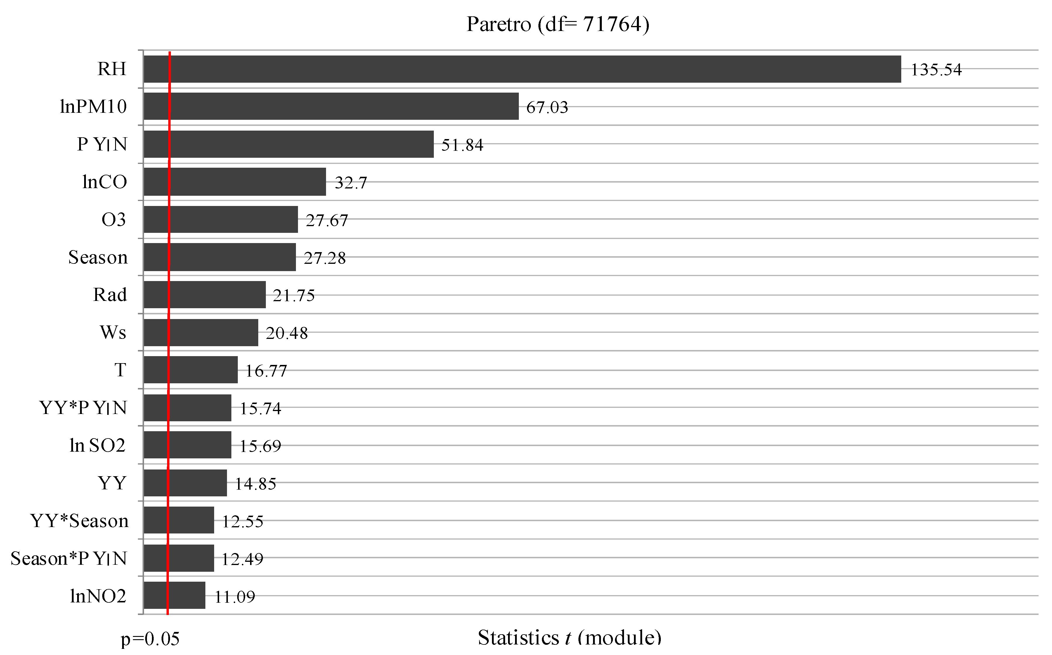
To picture the significance of the variables, they were ordered following the values of the Student’s
t-distribution for the assessment of the model parameter significance (
Figure 8—Pareto chart). The higher the
t-value was, the more important the significance of the factor was for explaining its influence on visibility. Relative air humidity and PM
10 were two most important factors affecting visibility on the basis of the identified model. The influence exerted by SO
2 and NO
2 on visibility was much lower from the impact that other analysed pollutants had. The results also show the influence of the seasonality, atmospheric precipitation (its presence or lack; variable: Prec.Y|N) and interactions between the periods (e.g., season * month) on visibility.
Figure 8.
Pareto chart for the significance of factors affecting visibility in the GRM.
Figure 8.
Pareto chart for the significance of factors affecting visibility in the GRM.
Table 8 presents estimated parameter values for the selected GRM (
Table 6 and
Table 7), together with estimations for the parameter errors,
t-distribution and p-value indicating the variable significance and coincidence with visibility. In a statistical sense, it was shown that the relative air humidity and wind speed variations corresponded with visibility more than the temperature. It was also revealed that visibility was most likely sensitive to the changes in the PM
10 and CO concentrations. Specifically, a 50% drop in the PM
10 concentration could be associated with visibility improvement by 2.9 km. On the other hand, a drop in the CO concentration by 50% corresponded with the visibility being increased by 2.2 km, however, there was no evidence for a direct cause-and-effect relationship. The 50% decrease in the O
3 concentration might only slightly affect the visibility increase, as suggested by the performed regression analyses.
Table 8.
Estimated parameter values for the selected GRM with estimations of parameter errors, t-distribution and p-value indicating the variable significance.
Table 8.
Estimated parameter values for the selected GRM with estimations of parameter errors, t-distribution and p-value indicating the variable significance.
| Regression Coefficien |
Level/Effect
|
Estimated Regression Coefficient
|
Estimated Standard Deviation
| t | p Value
|
|---|
| Intercept | | 82.615 | 0.633 | 130.468 | 0.000 |
| lnSO2 | | −0.902 | 0.057 | −15.692 | 0.000 |
| lnNO2 | | 0.827 | 0.075 | 11.089 | 0.000 |
| lnCO | | −3.122 | 0.095 | −32.699 | 0.000 |
| O3 | | −0.054 | 0.002 | −27.673 | 0.000 |
| T | | 0.097 | 0.006 | 16.766 | 0.000 |
| Ws | | 0.450 | 0.022 | 20.479 | 0.000 |
| RH | | −0.395 | 0.003 | −135.537 | 0.000 |
| Rad | | −0.005 | 0.000 | −21.751 | 0.000 |
| lnPM10 | | −4.220 | 0.063 | −67.032 | 0.000 |
| YY | 2004 | 0.727 | 0.163 | 4.467 | 0.000 |
| YY | 2005 | −0.736 | 0.164 | −4.495 | 0.000 |
| YY | 2006 | −1.829 | 0.168 | −10.867 | 0.000 |
| YY | 2007 | 0.880 | 0.175 | 5.024 | 0.000 |
| YY | 2008 | 0.913 | 0.165 | 5.540 | 0.000 |
| YY | 2009 | 2.028 | 0.137 | 14.847 | 0.000 |
| YY | 2010 | −1.619 | 0.162 | −9.997 | 0.000 |
| YY | 2011 | 1.174 | 0.115 | 10.182 | 0.000 |
| YY | 2012 | −0.287 | 0.142 | −2.016 | 0.044 |
| Season | warm | 1.695 | 0.062 | 27.284 | 0.000 |
| Prec.Y|N | Non-raining | 2.698 | 0.052 | 51.837 | 0.000 |
| Year * Season | 1 | 0.197 | 0.096 | 2.048 | 0.041 |
| Year * Season | 2 | −0.857 | 0.095 | −9.028 | 0.000 |
| Year * Season | 3 | −1.132 | 0.093 | −12.119 | 0.000 |
| Year * Season | 4 | −0.189 | 0.104 | −1.815 | 0.070 |
| Year * Season | 5 | −1.052 | 0.105 | −10.023 | 0.000 |
| Year * Season | 6 | −0.276 | 0.092 | −3.010 | 0.003 |
| Year * Season | 7 | 0.814 | 0.101 | 8.036 | 0.000 |
| Year * Season | 8 | 0.531 | 0.093 | 5.730 | 0.000 |
| Year * Season | 9 | 1.121 | 0.089 | 12.555 | 0.000 |
| Year * Prec.Y|N | 1 | 0.433 | 0.162 | 2.675 | 0.007 |
| Year * Prec.Y|N | 2 | 0.714 | 0.163 | 4.386 | 0.000 |
| Year * Prec.Y|N | 3 | −0.081 | 0.167 | −0.487 | 0.626 |
| Year * Prec.Y|N | 4 | 0.368 | 0.173 | 2.127 | 0.033 |
| Year * Prec.Y|N | 5 | −0.136 | 0.161 | −0.843 | 0.399 |
| Year * Prec.Y|N | 6 | 0.132 | 0.137 | 0.964 | 0.335 |
| Year * Prec.Y|N | 7 | 1.426 | 0.161 | 8.880 | 0.000 |
| Year * Prec.Y|N | 8 | −1.756 | 0.112 | −15.736 | 0.000 |
| Year * Prec.Y|N | 9 | −0.045 | 0.140 | −0.319 | 0.750 |
| Season * Prec.Y|N | 1 | 0.624 | 0.050 | 12.487 | 0.000 |
The results of the GRM analysis, performed herein, correspond with previous, abundant research, pointing that visibility degradation is due to particulate matter, as well as relative humidity, that can greatly enhance degradation in the presence of hygroscopic aerosols [
6,
17,
53].


 ,
, 


