1. Introduction
Atmospheric convection is involved in many of the central problems in meteorology and climate science [
1,
2]. Investigation and understanding of atmospheric convection is of great importance for the development and improvement of global weather and climate prediction [
3,
4]. Convection interacts with the larger-scale dynamics of planetary atmospheres in ways that remain poorly represented in global models [
5,
6]. The important role in the convective instability is played by the release of latent heat of condensation during phase transitions of water vapor in the moist saturated air [
7]. Many experimental and theoretical works, reviews and textbooks have been devoted to the thermal convection [
8,
9,
10,
11,
12]. Even so, we currently have not a complete understanding of this phenomenon.
According to Alekseev and Gusev [
13], the free convection can be of the two main types: The Rayleigh convection conditioned by the hypercritical vertical temperature gradient, and the lateral convection resulting from the temperature heterogeneity in horizontal plane. The interlatitude and the monsoonal type air circulations belong to the lateral convection. As for the classic Rayleigh vertical convection, the examples are the convection resulting in formation of the clouds distributed in space in form of cellular structures (Benard cells). Here, the vertical convection will be studied. For the analysis of a convective stability, the linearized system of equations describing thermal convection in a vertical plane has been solved by Rayleigh [
14]. It is valid to say that the Rayleigh theory is non-stationary two-dimensional linear analytical model of convection. The study of nonhydrostatic models commonly involves extensive numerical integrations. Such an approach was used by Ogura [
15], who studied the development of an axially symmetric moist convective cell toward the steady state. The numerical studies have been further developed by many authors (as, for example, in [
16,
17]). Much insight into the problem can be gained by using highly truncated models. Saltzman [
18] and Lorenz [
19] studied dry convection by only taking a few spectral components of the motion and temperature fields into account. They have developed the Rayleigh theory by considering the system of non-linear equations. However, they solved the obtained system of equations numerically. These studies have been followed by many others [
20,
21,
22]. When moist processes are considered, the formulation of a “low-order” model presents some special difficulties. These are due to the complex expressions for latent heat release and the asymmetric properties of condensation with respect to upward and downward motion. One simplified approach of the physics of condensation has been proposed by Shirer and Dutton [
23]. In their model, the condensation processes have the effect of modifying the critical Rayleigh number,
i.e., the critical vertical temperature gradient needed for the onset of convection. This model has been developed by Huang and Källén [
24] by considering the hysteretic effects. The effect of moisture is only introduced via condensational heating in [
24]. Low-order models of the atmosphere were also used to study specific problems such as blocking [
25]. Several particular solutions for inviscid non-heat-conducting atmosphere have been analyzed in [
26,
27,
28].
Currently, the numerical methods of analysis of nonstationary two- and three-dimensional non-linear models of convection with the use of high-performance computers are widely applicable in theoretical studies. On the other hand, because of their relative simplicity, low-order models present considerably more qualitative insight into the problem than the complicated numerical computations. In spite of this, it is of interest to obtain the analytical solution of stationary two-dimensional model of convection. It will allow us to understand better the fundamental nature of the atmospheric structures and dynamics. The obtained solution can be an effective tool at forecasting of convection parameters. Previously we have reported on the two-dimensional analytical model of dry air thermal convection [
29]. Here we present the further development of the two-dimensional analytical convection model which takes into account the atmospheric humidity. Hence, the purpose of this article is to define the conditions of the moist saturated air free convection occurrence within the framework of the two-dimensional convection model. Here we extend the classical parcel-based linear stability analysis to the case with a finite displacement.
2. Basic Equations of Moist Saturated Air Convection
Consider the ideal fluid equation of motion, in
x–z plane, in Eulerian form, in inertial reference system, neglecting the Earth rotation, in projections onto coordinates axes [
30,
31,
32]:
In equilibrium (statics):
Here ρi is the moist air parcel density; ρe the air parcel surrounding atmosphere density; and g the free fall acceleration. We accept the parameters of the surrounding atmosphere as an undisturbed state. Hence, the pressure may be written as: , here p′ is the pressure disturbance relative to the statics state.
In the moist atmosphere the air density equation in the Boussinesq approximation will be [
13]
where α = 1/
T0 is the air thermal expansion coefficient;
T0 = 273 K; Δ
T(
z) =
Ti(
z)–
Te(
z); Δ
T(
z) the overheat function;
Ti,
Te the air parcel internal and external temperatures;
s the water vapor mass fraction (also called specific humidity or moisture content); Δ
s=
si–
se the supersaturation function; β ≡
Md/
Mv–1 = 0.608;
Md = 29 g/mol the dry air molar mass;
Mv = 18 g/mol the water vapor molar mass. In other words, we assume that the density depends on temperature and vapor mass fraction and not depends on pressure [
33]. Here we do not consider the water loading.
The temperature change of the surrounding atmosphere will be considered to follow the law:
where γ is the surrounding air temperature gradient; and
Tec the surrounding air temperature at the condensation level (
zc). The moist saturated air temperature gradient is determined by [
34]
where γ
a is the dry-adiabatic temperature gradient;
L the specific heat of condensation;
cp the specific heat capacity at constant pressure;
sm the saturated vapor mass fraction. The quantity d
sm/d
z appearing in Equation (6) is a complicated function of temperature and pressure [
34]; this is why Equation (6) is usually analyzed numerically. To obtain an analytical solution, we should propose an adequate parametrization for the quantity d
sm/d
z. We specify the saturated vapor mass fraction change with altitude parametrically by expanding in a Taylor series:
here
K is some function of saturated vapor mass fraction at the condensation level (
smc).
Then for the moist-adiabatic temperature gradient we have the parametrical form:
here γ
mac is the moist-adiabatic temperature gradient at the condensation level [
34] (this is the known function of temperature and pressure).
Note that Equation (8) presents a linear approximation to the lapse rate. Analyzing and approximating the table values of the moist-adiabatic temperature gradient [
34], for the quantity ε we can get: ε =
LK/
cp ≈ 3·10
–7 °C/m
2.
Then we have that the temperature of the adiabatically rising moist saturated air parcel follows the law:
where
Tic is the rising air parcel temperature at the condensation level. The function
Ti(
z) graph presents the ’state curve’; the family of such curves is displayed on aerological diagrams. The table values of air temperature obtained from the state curve demonstrates the satisfactory agreement with the values calculated by Equation (9) within the convection layer of interest
zw –
zc ≤ 5 km. Here
zw is the convection level. Taking into account Equations (5) and (9) the overheat function will be:
where Δ
cT is the overheat function at the condensation level; Δγ
mac = γ – γ
mac is the difference of the ambient air temperature gradient and the rising air parcel temperature gradient at the condensation level. The quantity Δγ
mac determines the angle between the state curve and the stratification curve at the condensation level on the aerological diagram.
For the adiabatically rising air parcel the saturated vapor mass fraction follows the law:
Assume that the vapor mass fraction decreases linearly with altitude in the surrounding atmosphere:
where
sec is the water vapor mass fraction in the surrounding atmosphere at the condensation level;
b the vapor mass fraction gradient. Then for the supersaturation function we get
where Δ
cs =
smc –
sec is the supersaturation at the condensation level.
Taking into account Equations (10) and (13), Equation (4) for the air parcel density will be written as:
where
From here the level of equalization of the densities of the rising air parcel and surrounding air can be found:
The level of equalization of the temperatures (the level of neutral buoyancy) is determined by
The steady motion of air parcel is described by the set of equations of the moist saturated air convection:
In Equation (19) the following assumption has been made:
To satisfy Equation (23), in the present study we seek the analytical solution for the pressure disturbance in the form:
where
is some level determined below.
Substituting Equations (20) and (21) into Equation (19), we finally get the set of equations of moist saturated air free convection in the form:
Further we will find the solution of the obtained system of equations.
3. Solution of the Moist Saturated Air Convection Equations
It follows from the continuity Equation (27) that for the shallow convection condition the stream function ψ may be introduced [
30,
31,
32]:
Substituting Equation (28) into Equations (25) and (26), we get:
Equation (30) can be written as
where
is the square of the Brunt–Väisälä frequency for the moist saturated air;
We seek solution of the resulting equations set in the following form:
Substituting Equation (34) into Equation (29), we get:
Substituting Equation (34) into Equation (31), we obtain:
From Equation (36), separating the variables, it follows that:
where
k is the constant requiring determination. The Equation (37) solution has the form:
We seek the Equation (38) solution with the following form:
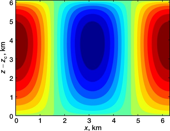
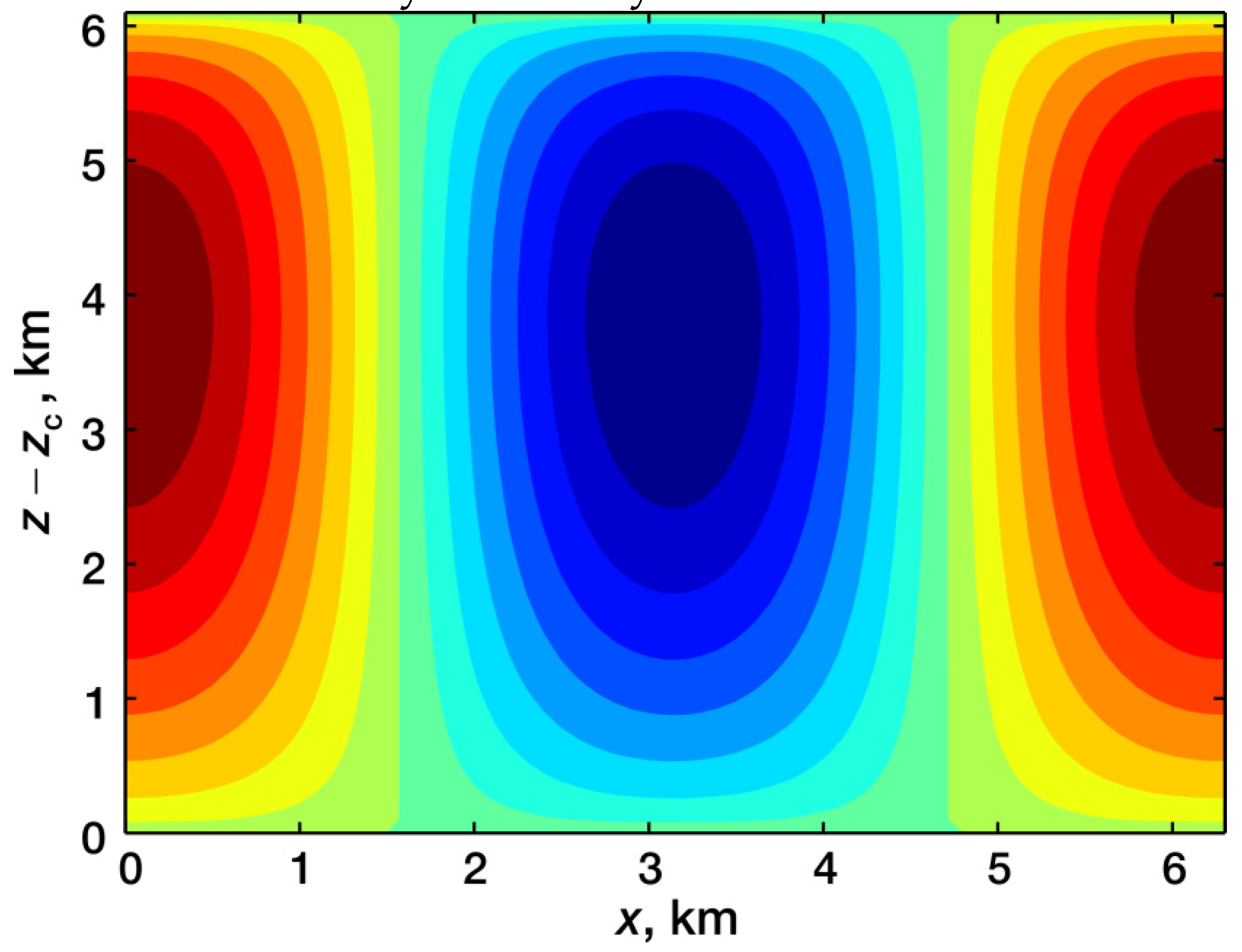
Substituting Equation (41) directly into Equation (38), we see that the solution is valid. Hence, for the stream function, we have the expression:
Figure 1 shows this function graph. As is seen, the stream function is symmetrical in horizontal direction and asymmetrical in vertical direction. The level of maximal vertical velocities is in the upper part of the convective cell contrary to the dry and moist unsaturated air convection [
29].
Figure 1.
Stream function at b = 10–6 m–1, ΔcT = 0.5 °C, Δcs = 0, Δγmac = 5 × 10⁻⁴ °C/m, ε = 3 × 10⁻⁷ °C/m2, k = 10–3 m–1, .
Figure 1.
Stream function at b = 10–6 m–1, ΔcT = 0.5 °C, Δcs = 0, Δγmac = 5 × 10⁻⁴ °C/m, ε = 3 × 10⁻⁷ °C/m2, k = 10–3 m–1, .
From Equations (28) the velocity projections can be written:
From here, using the condition
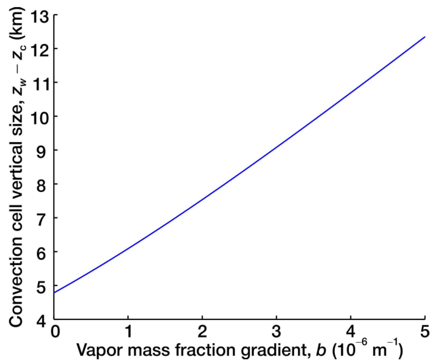
w = 0, we get the expression for the vertical size of convection cell (or cloud size):
Figure 2 shows the dependence of the convection cell vertical size on the water vapor mass fraction gradient. As is seen, the convection cell vertical size rises monotonically with the vapor mass fraction gradient.
Figure 2.
Convection cell vertical size
vs. water vapor mass fraction gradient. The atmospheric parameters are the same as in
Figure 1.
Figure 2.
Convection cell vertical size
vs. water vapor mass fraction gradient. The atmospheric parameters are the same as in
Figure 1.
4. Analysis and Discussion of the Obtained Solution
We find the maximal velocities level from the condition: ∂
w/∂
z = 0. Taking the derivative of Equation (44) with respect to
z, we get:
If
(the overheat Δ
cT and the oversaturation Δ
cs are equal to zero at the condensation level), then for the convection level and for the maximal velocities level we have
From here one can see that the maximal velocities level is not in the center of the convective cell as it has been for the dry air convection. The maximal velocities level for the moist saturated air is at 2/3 of the vertical size of convection cell.
Substituting the expression for
zmax –
zc into Equation (44), we get for the ascending moist saturated air maximal velocity the equation:
If
, then we have
Let us find the pressure spatial distribution. For this, integrating Equation (35), we get:
The constant of integration can be found from the condition that at the maximal velocities level the pressure disturbance is equal to zero at the points meeting the condition cos
2kx = 1. From here we have
Here we take into account that if
, then
From here, taking into account Equation (24) and assuming
, for the pressure disturbance we get
It should be noted that the analytical solution Equation (42) is obtained by integrating only one Equation (36); in so doing we neglected the term in accordance with the condition Equation (23). In such an approach to the problem, Equation (18) plays a role of auxiliary equation for the pressure disturbance determination. To make Equations (18) and (19) agree with condition Equation (23) we were compelled to consider Equation (18) at the point of maximal velocities where the pressure disturbance is equal to zero.
5. Conclusions
Hence, we have obtained the new solution of the equations of moist saturated air convection in the atmospheric cloud layer. The solution is obtained within the framework of the stationary 2D analytical model. It has been shown that the convection parameters in moist atmosphere strongly depend on the water vapor mass fraction gradient. The expression for the convective cell vertical size is obtained.
The obtained solutions can be valuable in the convection parameters forecasting practice. As it can be seen from obtained equations, the important convection parameters, such as convection level, level of neutral buoyancy, maximal velocities level, and maximal velocity itself, are determined by the characteristics which can be calculated from aerological diagrams using radiosounding data. These characteristics are the angle between the state curve and the stratification curve at the condensation level and the water vapor mass fraction gradient.


