Article

Joint Inversion of Atmospheric Refractivity Profile Based on Ground-Based GPS Phase Delay and Propagation Loss

College of Meteorology and Oceanography, PLA University of Science and Technology, Nanjing 211101, China
*
Author to whom correspondence should be addressed.
These authors contributed equally to this work.
Submission received: 23 November 2015 / Revised: 23 December 2015 / Accepted: 13 January 2016 / Published: 21 January 2016

Abstract

:
In this paper, we present a new estimation of the atmospheric refractivity profile combining the scattering signal (electromagnetic wave propagation loss) and the direct signal (phase delay). The refractivity profile is modeled using four parameters, i.e., the gradient of the refractivity profile (c1, c2) and the vertical altitude (h1, h2). We apply the NSGA-II (Non-dominated Sorting Genetic Algorithm II), a multiobjective optimization algorithm, to achieve the goals of joint optimization inversion in the inverting process, and compare this method with traditional individual inversion methods. The anti-noise ability of joint inversion is investigated under the noiseless condition and adding noise condition, respectively. The numerical experiments demonstrate that joint inversion is superior to individual inversion. The adding noise test further suggests that this method can estimate synthesized parameters more efficiently and accurately in different conditions. Finally, a set of measured data is tested in the new way and the consequence of inversion shows the joint optimization inversion algorithm has feasibility, effectiveness and superiority in the retrieval of the refractivity profile.

1. Introduction

The atmospheric duct is a refraction phenomenon that occurs in the atmosphere where there are larger negative refractive gradient values, causing electromagnetic waves to be bent out of the transmitting direction. The atmospheric duct is able to affect the performance of the electromagnetic communication system severely, for example as in a radar system designed and evaluated by the standard model of atmospheric refractivity. Therefore, making full use of the information carried by electromagnetic waves to retrieve the atmospheric duct has become a new subject in the field of inverse problems [1,2]. Krolik and Tabrikian [3] first proposed a method of using radar clutter data to obtain the atmospheric refractivity profile. Since then, many scholars have enriched the inversion method using radar echo to invert the atmospheric duct, including the genetic algorithm [4], the Bayesian-Markov chain Monte Carlo method (MCMC) [5], and the Support Vector Machine (SVM) [6], etc. [7,8,9]. However, these methods have many drawbacks, such as low detecting precision, high equipment costs, vulnerability to electromagnetic interference or electromagnetic exposure, and so on.
With the development of ground-based GPS (Global Positioning System), Lowry et al. [10] and Sheng et al. [11] put forward a new method whereby the ground-based GPS delay was used to retrieve the atmospheric refractivity profile. Even so, the inversion effect was not ideal because it only used delay information. Xue et al. [12] tried to improve the inversion accuracy by increasing the vertical resolution of the inversion model, but the difference between the retrieved results and the observation was still obvious at a low level. These retrieved results were calculated from the single observation. Wu et al. [13] tried using the phase delay and bending angle to retrieve the refractivity profile and obtained a relatively accurate result. However, this method did not highlight the superiority of joint inversion due to the strong correlation between the two observations.
Joint inversion is a method using multiple observations to estimate the synthesized parameters, and it plays an important role in the field of geophysical quantitative analysis, especially in geological exploration, oil and gas exploration, etc. [14,15]. Alekseev et al. [16] described the solution to joint inversion problems and their general characteristics in detail. They concluded that joint inversion has more advantages than a single geophysical data inversion. Lin et al. [17] and Chen et al. [18] demonstrated that the joint inversion method is able to improve the inverting accuracy through comparing retrievals and observations.
There are two types of joint inversion thoughts, generally [19]. The first kind is based on geophysical observation with the same physical characteristics, for example as in the joint inversion with phase delay and bending angle proposed by Wu et al. [13]. The two kinds of information have such a strong relationship that they can be regarded as the same data expressed in two different forms. The other joint inversion thought is based on independent geophysical observation which has different physical characteristics. This inversion thought usually brings good results and is a perfect choice in geophysical inversion. Nevertheless, this thought has not been documented in the field of atmospheric duct retrieval yet. Therefore, in this paper, we will propose a new inversion method to retrieve the atmospheric refractivity profile using independent geophysical observations based on the second inversion thought.
The organization of the remainder of this paper is detailed below. Section 2 outlines the forward model and parameterization schemes. This section focuses on introducing the phase delay and propagation loss model in the forward process, and builds a four-parameter profile model. The selected algorithm is described in Section 3. The analysis and results of the numerical experiments (including the parameter settings) are given in Section 4. Meanwhile, we also present the performance of the novel method in real conditions. The conclusions and the direction of possible future research are presented in Section 5.

2. Forward Model and Parameterization Schemes

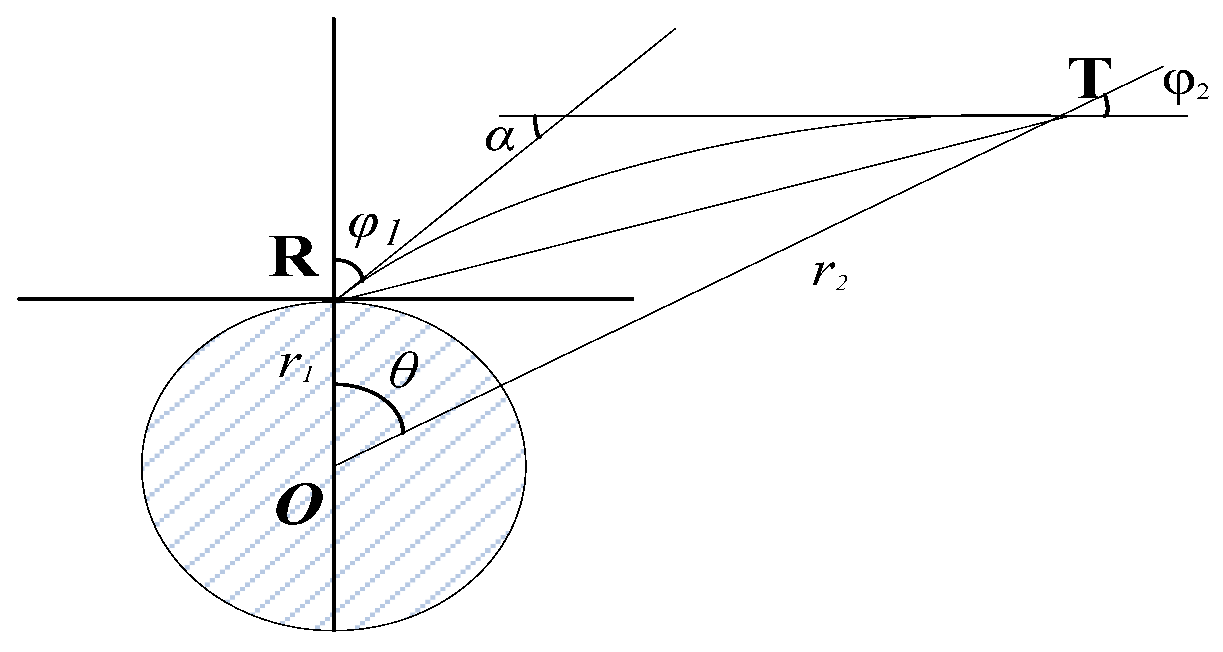
2.1. Forward Model-Excess Phase Delay

In the earth's atmosphere, ground-based GPS signals will delay as a result of the refractivity gradient. According to the refractivity formula proposed by Smith and Weintraub [20]:
N = 77.6 P / T + 3.73 × 10 5 e / T 2 = ( n 1 ) × 10 6
where P and e are the atmospheric and water vapor pressures in hectopascal, T is the atmospheric temperature in Kelvin, and N is the refractivity in N-unit, n is the refractivity index in dimensionless.
d M / d z = d N / d z + 0.157
Here, dN/dz is the refractivity gradient in N-unit/Km and dM/dz is the modified refractivity gradient in M-unit/Km. M and N could be transformed into each other by Equation (2). dN/dz is always regarded as the standard of classifying the atmospheric condition. A region with a positive refractivity gradient is called sub-refraction, where radio waves escape from the Earth’s surface. In these regions with a negative refractivity gradient, rays are always bent toward the Earth. The region with a refractivity gradient of between −76 N-unit/Km and 0 N-unit/Km is defined as normal refraction. When the value of dN/dz is between −76 N-unit/Km and −160 N-unit/Km, this condition is classified as super-refraction. If the gradient value is less than −160 N-unit/Km, the atmospheric duct occurs. The atmospheric duct always leads to rays curving down into the surface at low altitudes.
Using the hypothesis of a spherical, radially symmetrical refractive medium, the ground-based GPS signal delay in neutral atmosphere can be calculated using the means of the path integral [11].
S = r 1 r 2 n ( r ) d l
where dl can be defined as d l = d r 2 + r 2 d θ 2 . As Figure 1 shows, O is the geocenter, R and T represent the receiver and transmitter, r1 and r2 are the distances from the geocenter to receiver and transmitter, respectively. Using Snell's law and substituting dr = dl cosα, the phase delay can be expressed as:
S = x 1 x 2 r 2 n / r 2 n 2 a 2 d r = x 1 x 2 ( 1 x d m d x ) x / x 2 a 2 d x
Here, x = rn(r) denotes the refractive radius and m(x) = ln(n(x)). The propagation path of a ground-based GPS signal in a vacuum can be represented as:
S = r 1 2 + r 2 2 2 r 1 r 2 cos θ
The spherical angle θ is the central angle and can be expressed as θ = ϕ1ϕ2 + α, where ϕ1 and ϕ2 is the zenith of the ray, α is the bending angle. Thus, we can obtain the excess phase delay from the given refractivity index profile n(r):
Δ S = S S
Figure 1. Diagram of GPS radio signal propagation.
Atmosphere 07 00012 g001

2.2. Forward Model-Propagation Loss

The electromagnetic wave propagation equation (Helmholtz equation) is usually replaced by the terrain parabolic equation [5]. Establishing a local rectangular coordinate system where the x-axis is the ground horizontal distance and the z-axis is altitude, the parabolic equation of electromagnetic wave propagation can be expressed as:
z 2 u + 2 i k x u + k 2 ( M 2 1 ) u = 0
Here, k is the wave number in free space; M is the modified refractivity in M-unit; z and x represent the distance from the vertical direction and horizontal direction to the origin, respectively. The boundary condition of the parabolic equation can be reviewed in reference [8]. For a parabolic equation with an initial value, the ‘step by step’ numerical method is suggested to solve the problem, namely to give an efficient solution at a certain distance x0. Using the Fourier ‘split-step’ solution to calculate all the results of x > x0, the following observing formula is obtained:
h ( x , M ) = 2 L ( x , M ) + 10 log 10 ( x ) + C
in which L(x,M) is the single-way propagation loss of the ground-based GPS signal, C represents all the constant parameters and h(x,M) is the receiving power density of ground-based GPS signals. If h(x,M) and other related parameters are known, the propagation loss of electromagnetic wave L(x,M) can be obtained from Equation (8).

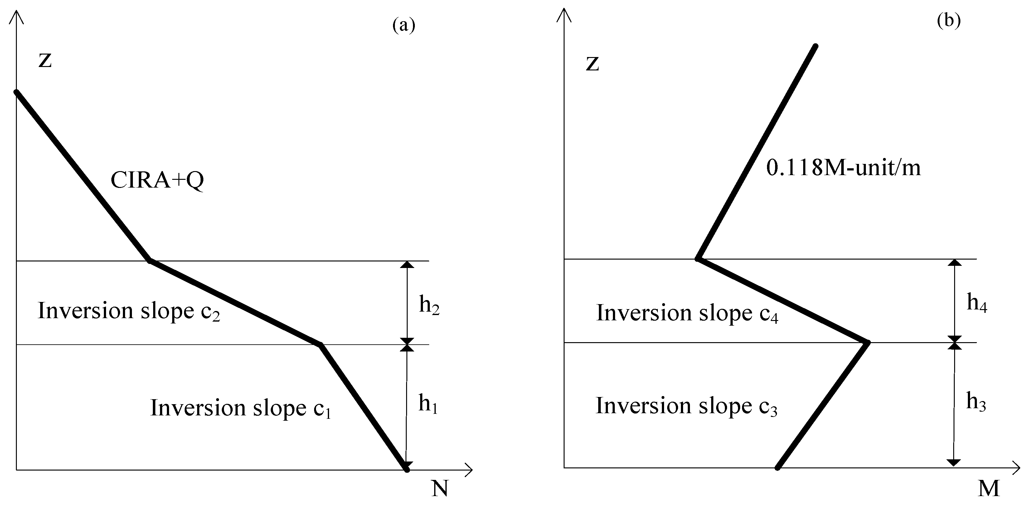
2.3. Four-Parameter Model

As shown in Figure 2a, a coordinate system where the refractivity N is the horizontal axis and the vertical altitude z is the vertical axis is established and the refractivity profile in the phase delay model is constructed [10]. c1 is the gradient of the refractivity profile from the receiver to the altitude h1 which is a variable parameter, and c2 is the gradient of the refractivity profile from the altitude h1 to the altitude h1 + h2 which is always larger than 160 N-unit/Km. The gradient of the refractivity profile from altitude h1 + h2 to an altitude of 6 Km can be obtained from the CIRA + Q model (The CIRA86a with Q_UoG model) [21].
Using the propagation loss model, a coordinate system where the modified refractivity M is the horizontal axis and the vertical altitude z is the vertical axis is established and the refractivity profile is constructed. In Figure 2b, there is a three-section parameter scheme which can be described by a segmented function.
M ( Z ) = M o + { c 3 z c 3 h 3 + c 4 ( z h 3 ) c 3 h 3 + c 4 h 4 + 0.118 z z < h 3 h 3 < z < h 3 + h 4 z > h 3 + h 4
c3 is the gradient of the modified refractivity profile from the receiver to the altitude h3 and c4 is the gradient of the modified refractivity profile from the altitude h3 to the altitude h3 + h4. The atmosphere above h3 + h4 is always regarded as the standard situation.
In order to combine the four-parameter model (phase delay model and propagation loss model) to retrieve the synthesized parameters (c1, c2, h1, h2), Equation (2) will transform M into N and we will change the inputting parameters of the propagation loss model accordingly in the process of joint inversion.
Figure 2. Four-parameter geometric scheme of the atmospheric profile.
Atmosphere 07 00012 g002

3. Inversion Algorithm

The joint inversion with phase delay and propagation loss is a multiobjective optimization process. Therefore, it is necessary to find a multiobjective optimization algorithm to realize this new method. In this paper, the NSGA-II is chosen to achieve this goal. This optimization algorithm is an improved algorithm based on the NSGA (the Non-dominated Sorting Genetic Algorithm) proposed by Srinivas and Deb in 2000 [22,23]. The NSGA-II improves the operation speed and robustness of the algorithm, gradually becoming a benchmark of the other multiobjective optimization algorithm.
It is assumed the vector x = (c1,c2,h1,h2)T, and the cost functions are defined as:
{ J 1 ( x ) = ( Δ S ( x ) obs Δ S ( x ) mod ) 2 = min ! J 2 ( x ) = ( h ( x ) obs h ( x ) mod ) 2 = min !
The NSGA-II is used to globally search the best parameters fitting into Equation (10). For all test problems, the parameter settings of NSGA-II are as follows: the number of iterations is set at 200, the population is 200, the number of the objective function is 2, and the crossover and mutation parameters are set to 20. The variables are treated as real numbers, and we adopt the simulated binary crossover (SBX) and the real parameter operator in the experiment [22].

4. Results

To verify the feasibility and anti-noise ability, two inverted numerical simulations and one real data inversion test are considered. The first simulated condition does not add any disturbance, and the second simulation adds 3%, 5%, 7%, and 10% Gaussian white noise, respectively. Based on the real situation, we designed a series of parameter settings in the simulation. The detailed test processes are as follows.

4.1. Ideal Condition

In order to calculate the fitness of cost functions, the boundary of inverting parameters is set as Table 1 and the antenna is adjusted for 18 m. The elevation angle is 1°. In fact, appropriate boundary setting has a significant influence on the precision of the inversion results. To contrast the performance of joint inversion, this paper uses the traditional general GA (the Genetic Algorithm) [24] to process the single objective optimization inversion. Parameter settings for the GA are as follows: the number of iterations is set at 200, and the population is 200, consistent with the multiobjective inversion setting. The single point crossover rate is set from 0.9 to 0.3 with linear decline, and single point mutation rate is set from 0.01 to 0.1 with linear growth. In order to compare fairly, the upper and lower bounds of each individual inversion parameter are the same as the joint inversion. In Table 1, there are inversion results of synthesized parameters in the ideal condition, namely adding 0% Gaussian noise.
As seen in Table 1, the synthetic parameters inverted by the NSGA-II are better than the compared algorithms in the ideal condition. The established parameters of propagation loss are partly superior to the phase delay in GA, especially the refractivity gradient c1.
Table 1. The value of inversion parameters under noiseless and adding noise condition.
ParametersInversion Slope c1Height h1Inversion Slope c2Height h2
UnitsN-units/mmN-units/mm
Lower Bound−0.150−0.4250
Upper Bound01500350
True Value−0.02100−0.2300
NSGA-II0%−0.0227 (13.5%)99.8246 (−1.75%)−0.199 (−0.5%)298.7839 (−0.4%)
3%−0.0155 (−22.5%)95.9541 (−4.04%)−0.1990 (−0.5%)306.0764 (2.03%)
5%−0.0121 (−39.5%)94.7610 (−5.239%)−0.2008 (0.4%)306.0295 (2.01%)
7%−0.0254 (27%)98.9927 (−1.007%)−0.2007 (0.35%)300.4304 (0.143%)
10%−0.0146 (−27%)89.1687 (−10.83%)−0.1959 (−2.05%)302.2124 (0.74%)
GA-Delay0%−0.0576 (188%)109.5935 (9.59%)−0.1969 (−1.55%)281.8778 (−6.04%)
3%−0.0519 (159.50%)91.2888 (−8.71%)−0.1723 (−13.85%)332.9521 (10.98%)
5%−0.0361 (80.50%)115.5426 (15.54%)−0.1865 (−6.75%)305.7128 (1.90%)
7%−0.0985 (392.50%)140.5176 (40.52%)−0.1665 (−16.75%)328.5602 (9.52%)
10%−0.0618 (209.00%)124.9692 (24.97%)−0.1693 (−15.35%)273.2624 (−8.91%)
GA-Loss0%−0.0208 (4%)96.0873 (−3.91%)−0.1948 (−2.6%)309.6933 (3.23%)
3%−0.0181 (−9.50%)102.2168 (2.22%)−0.2050 (2.50%)296.1529 (−1.28%)
5%−0.0198 (−1.00%)93.3431 (−6.66%)−0.1897 (−5.15%)312.0424 (4.01%)
7%−0.01934 (−3.30%)97.9463 (−2.054%)−0.1905 (−4.75%)307.5467 (2.52%)
10%−0.0293 (46.50%)113.9005 (13.90%)−0.2106 (5.30%)262.6215 (−12.46%)
Figure 3 shows the refractivity profile and the corresponding absolute deviation. The absolute deviation profile reflects the difference between inversion and simulation. First of all, in the near-ground atmosphere, the deviation between joint inverting values and simulation is less by a margin of 1 N-units, and perfect inversion results have been achieved. Secondly, the individual inversion of propagation loss is relatively good, having a maximal absolute deviation of less than 2 N-units, whereas inversion results based on phase delay are the worst. In general, joint inversion contributes to superior performance which individual inversion does not present in the ideal case.
Figure 3. The retrievals with different Gaussian noise: (a) and (b) are the refractivity profile and corresponding refractivity deviation by NSGA-II; (c) and (d) are the refractivity profile and corresponding refractivity deviation by GA-Delay; (e) and (f) are the refractivity profile and corresponding refractivity deviation by GA-Loss.
Atmosphere 07 00012 g003

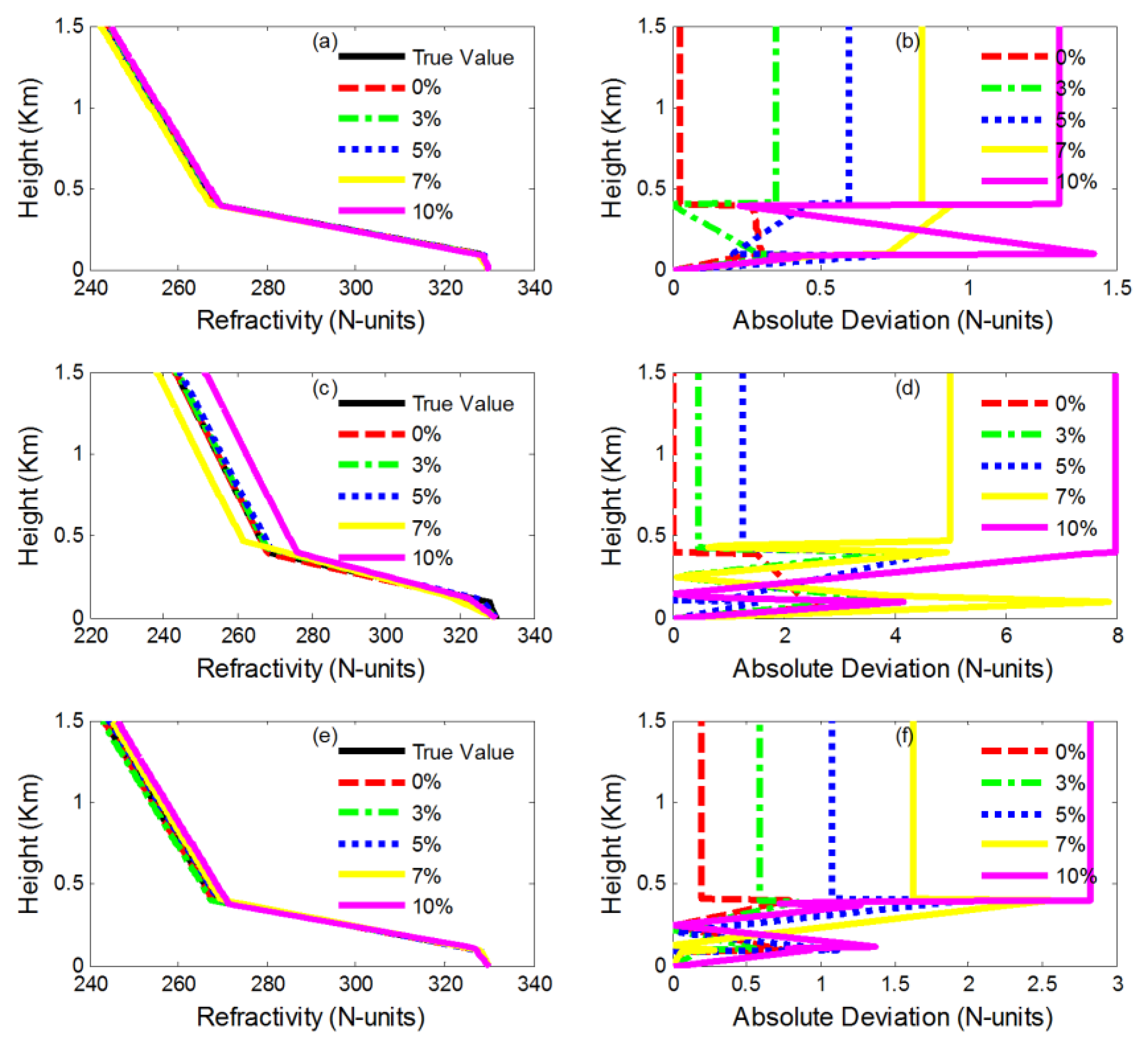
4.2. Adding Gaussian Noise

In the actual observation, ground-based GPS data usually contains a lot of white noise. This section considers the influence of measurement noise to the performance of joint inversion. Here, this paper successively adds 3%, 5%, 7% and 10% random Gaussian noise to simulate real data in the experiments. Table 1 gives the inversion values of parameters in the various noise environments and the percentages of relative deviation are in the parentheses.
As Table 1 shows, retrievals from phase delay by GA (GA-Delay) are greatly influenced by the noise. The inverting parameter is not as good as the estimation of joint inversion and propagation loss by GA (GA-Loss). In contrast, the established parameters of propagation loss are obviously better than other methods except for when adding the 10% noise condition, in which the NSGA-II shows the best performance. However, optimal parameter inversion does not mean the inverting profile converges to the real profile more closely. In fact, as seen from the refractivity profile of Figure 3, the joint inversion possesses the best convergence in all the adding noise conditions, and the difference between the retrieval of the phase delay by GA and the true value is the largest. Thus, we can conclude joint inversion has strong noise immunity according to the performance of different inversion methods.

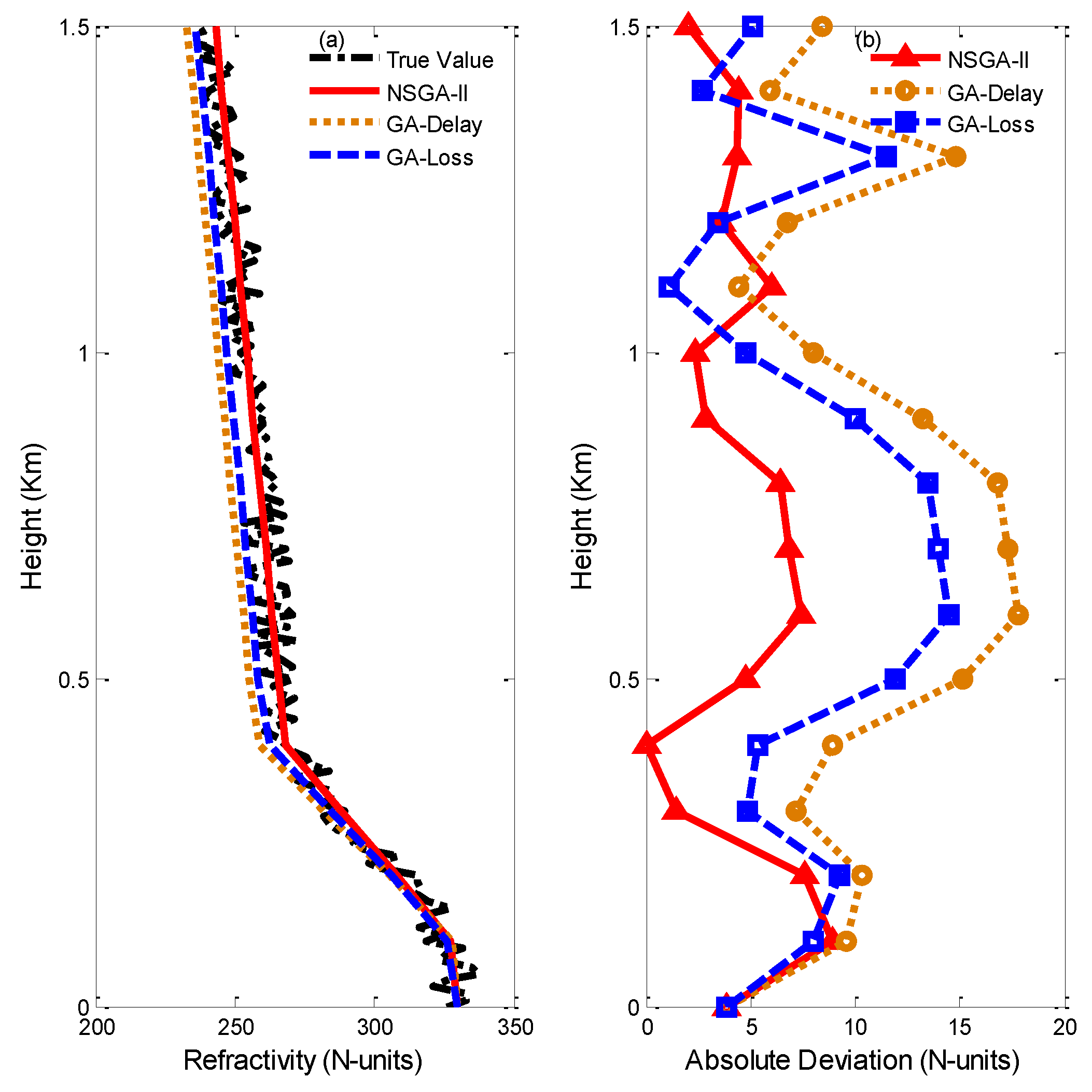
4.3. Real Data Testing

In order to further test the performance of joint inversion, real GPS data is used. True ground-based GPS observation data from the observation at Jiangxi Poyang Lake (115.27°E, 29.11°N), the corresponding sounding data from the meteorological rocket detection data (~4 m sampling at altitudes < 1.5 Km) and low resolution radiosondes (~50 m sampling at altitudes < 6 Km) were obtained, and the observation time was 17 April 2009. There is one observation in total. The excess phase is estimated using a modified version of Bernese v5.0 software in a precise point positioning mode [11], and the propagation loss is calculated according the receiving power density of the antenna. Table 2 depicts the results of inversion parameters by different inverting methods.
Table 2. The value of inversion parameters by different inversion methods.
ParametersInversion Slope c1Height h1Inversion Slope c2Height h2
UnitsN-units/mmN-units/mm
NSGA-II−0.0281105.0418−0.2013293.8846
GA-Delay−0.0212102.3759−0.2313304.9078
GA-Loss−0.0374110.5404−0.2187298.8363
Figure 4. Inversion results of NSGA-II and GA. (a) The refractivity profile. (b) The corresponding refractivity deviation.
Atmosphere 07 00012 g004
It is shown in Figure 4 that when real GPS data are used, because real data contain some observation deviations, the inversion effect is not as perfect as that of simulated data. Nevertheless, the absolute deviation is still kept within modest bounds. Since the model of four parameters and the observations have defects, there is a deviation between real sounding data and inversion, and the inverting profile still has a low ability to depict the real atmospheric refractivity environment. Therefore, the next focus of our study is improving the model and providing a better algorithm. Overall, based on the results of inversion, we can know that the joint inversion is relatively successful, and the refractivity structure and characteristics aremanifested well.

4.4. Feasibility

To examine the feasibility of joint inversion at a higher antenna altitude, the antenna altitude is adjusted to 400 m or 600 m. The elevation angle is set to 1°. Table 3 gives the inversion results. As shown in Table 3, some parameters inverted by NAGA-II are obviously worse than those inverted by GA, while the others are inverted perfectly by NSGA-II. In other words, it is difficult to determine which method is superior if we only estimate from the inverting parameters. Due to this reason, Figure 5 gives the absolute deviation profile.
Table 3. The value of inversion parameters.
ParametersInversion Slope c1Height h1Inversion Slope c2Height h2
UnitsN-units/mmN-units/mm
True Value−0.051100−0.3300
400 mNSGA-II−0.0501 (0.20%)1058.2 (−3.80%)−0.35 (16.67%)312.6988 (4.23%)
GA-Delay−0.05 (0.0%)1053.1 (−4.26%)−0.3029 (0.97%)309.7630 (3.25%)
GA-Loss−0.0503 (0.60%)1148.4 (4.40%)−0.2723 (−9.23%)304.0592 (1.35%)
600 mNSGA-II−0.05 (0.0%)1028.82 (−6.40%)-0.41 (36.70%)289.8588 (−3.38%)
GA-Delay−0.044 (-12.00%)1012.1 (−7.99%)-0.4659 (−55.30%)293.7786 (−2.07%)
GA-Loss−0.05 (0.0%)1029.8588 (−6.38%)-0.2508 (−16.40%)311.7714 (3.92%)
Figure 5. Refractivity absolute deviation under different antenna height: (a) 400 m antenna height. (b) 600 m antenna height.
Atmosphere 07 00012 g005
As Figure 5 shows, obviously, the joint inversion results are not ideal and the difference between the two profiles is larger. In contrast, the results of individual inversion based on a single observation are relatively good and properly depict the real structure of the atmospheric refractivity. This phenomenon further illustrates that joint inversion has some limitations in the higher antenna condition.
In fact, combining Figure 5 with Figure 3, it is also easily found that the result of individual inversion is worse than that of low height. That means the antenna altitude has a profound effect on the inversion indeed.

5. Conclusions

In this paper, an improved retrieval method is proposed combining GPS scattering signals and GPS direct signals to estimate the synthesized parameters of atmospheric refractivity. The inverting refractivity profile can be more perfectly estimated by joint inversion than by using a single observation to retrieve it. In the estimation, traditional GA is chosen to test the performance of joint inversion in the ideal condition, the Gaussian noise case, and the real situation, respectively. Under different noise conditions, the estimated results demonstrate that joint inversion has a higher accuracy and the inverting profile converges to the simulated value more closely than the compared methods. Although a large deviation exists, the measured data testing shows joint inversion is qualified for depicting a real refractivity profile. Nevertheless, joint inversion still has some limitations in the case of a higher antenna which may be attributed to the suitable altitude of the propagation loss model. Finally, this paper does not consider the effect of elevation angle on joint inversion. This problem will be one direction of the future research work.

Acknowledgments

This research was supported by National Natural Science Foundation of China (41375028). We are grateful to the editors and anonymous reviewers for their constructive comments on the earlier version of the manuscript.

Author Contributions

Zheng Sheng and Hanqing Shi conceived and designed the research; Qixiang Liao performed the experiments; Zheng Sheng and Hanqing Shi analyzed the data and Qixiang Liao wrote the manuscript.

Conflicts of Interest

The authors declare no conflict of interest.

Abbreviations

The following abbreviations are used in this manuscript:
GA:
The traditional general genetic algorithm
GA-Delay:
Retrieval from phase delay by GA
GA-Loss:
Retrieval from propagation loss by GA

References

  1. Zhao, X. Source localization in the duct environment with the adjoint of the PE propagation model. Atmosphere 2015, 6, 1388–1398. [Google Scholar] [CrossRef]
  2. Zhang, J.P.; Wu, Z.S.; Zhao, Z.W.; Zhang, Y.S.; Wang, B. Propagation modeling of ocean-scattered low-elevation GPS signal for marine tropospheric duct inversion. Chin. Phys. B 2012, 21. [Google Scholar] [CrossRef]
  3. Krolik, J.L.; Tabrikian, J. Tropospheric refractivity estimation using radar clutter from the sea surface. SPAWAR Sys. Command. Tech. Rep. 1997, 2989, 635–642. [Google Scholar]
  4. Gerstoft, P.; Rogers, L.T.; Krolik, J.L.; Hodgkiss, W.S. Inversion for refractivity parameters from radar sea clutter. Radio Sci. 2003, 38. [Google Scholar] [CrossRef]
  5. Sheng, Z. The estimation of lower refractivity uncertainty from radar sea clutter using the Bayesian-MCMC method. Chin. Phys. B 2013, 22. [Google Scholar] [CrossRef]
  6. Douvenot, R.; Fabbro, V.; Gerstoft, P.; Bourlier, C.; Saillard, J. A duct mapping method using least squares support vector machines. Radio Sci. 2008, 43. [Google Scholar] [CrossRef] [Green Version]
  7. Wen, D.B.; Yuan, Y.B.; Ou, J.K.; Zhang, K. Ionospheric response to the geomagnetic storm on 21 Augus 2003 over China using GNSS-based tomographic technique. IEEE Trans. Geosci. Remote Sens. 2010, 48, 3212–3217. [Google Scholar]
  8. Yardim, C.; Gerstoft, P.; Hodgkiss, W.S. Tracking refractivity from clutter using Kalman and particle filters. IEEE Trans. Antennas Propag. 2008, 56, 1058–1070. [Google Scholar] [CrossRef]
  9. Sheng, Z.; Wang, J.; Zhou, S.; Zhou, B.H. Parameter estimation for chaotic systems using a hybrid adaptive cuckoo search with simulated annealing algorithm. Chaos 2014, 24. [Google Scholar] [CrossRef] [PubMed]
  10. Lowry, A.R.; Rocken, C.; Sokolovskiy, S.V.; Anderson, K.D. Vertical profiling of atmospheric refractivity from ground-based GPS. Radio Sci. 2002, 37. [Google Scholar] [CrossRef]
  11. Sheng, Z.; Fang, H.X. Monitoring of ducting by using a ground-based GPS receiver. Chin. Phys. B 2013, 22, 575–579. [Google Scholar] [CrossRef]
  12. Wu, X.; Wang, X.; Lü, D. Retrieval of vertical distribution of tropospheric refractivity through ground-based GPS observation. Adv. Atmos. Sci. 2014, 31, 37–47. [Google Scholar] [CrossRef]
  13. Wu, Y.Y.; Hong, Z.J.; Guo, P.; Zheng, J. Simulation of atmospheric refractive profile retrieving from low-elevation ground-based GPS observation. Chin. J. Geophys. 2010, 53. [Google Scholar] [CrossRef]
  14. Miller, E.L.; Abriola, L.M.; Aghasi, A. Environmental remediation and restoration: Hydrological and geophysical processing methods. IEEE Signal Process. Mag. 2012, 29, 16–26. [Google Scholar] [CrossRef]
  15. Liu, J.; Liu, Q.H.; Li, J.; Ma, H.Z.; Yang, L.; Du, H.J. Radiant directionality modeling of joint thermal infrared and microwave for typical crops. J. Remote Sens. 2014, 18. [Google Scholar] [CrossRef]
  16. Alekseev, A.S. Quantitative statement and general properties of solutions of cooperative inverse problems (integral geophysics). In Proceedings of the 1991SEG Annual Meeting, Houston, TX, USA, 10–14 November 1991.
  17. Lin, W.; Xiao, P.K.; Houtse, H.; Jian, F.; Cheng, Y.X.; Yong, W. Joint gravity and gravity gradient inversion for subsurface object detection. IEEE Geosci. Remote Sens. Lett. 2013, 10, 865–869. [Google Scholar] [CrossRef]
  18. Chen, H.G.; Li, J.X.; Wu, J.S.; Yu, P. Study on simulated-annealing MT-gravity joint inversion. Chin. J. Geophys. 2012, 55, 663–670. [Google Scholar]
  19. Yang, H.; Dai, S.K.; Song, H.B.; Huang, L.P. Overview of joint inversion of integrated. Geophys. Pro. Geophy. 2002, 17, 262–271. [Google Scholar]
  20. Guo, P.; Kuo, Y.H.; Sokolovskiy, S.V.; Lenschow, D.H. Estimating atmospheric boundary layer depth using COSMIC radio occultation data. J. Atmos. Sci. 2011, 68, 1703–1713. [Google Scholar] [CrossRef]
  21. Kirchengast, G.; Hafner, J.; Poetzi, W. The CIRA86aQ_UoG Model: An Extension of the CIRA-86 Monthly Tables Including Humidity Tables and a Fortran95 Global Moist Air Climatology Model; IMG/UoG technical report; ESA/ESTEC: Graz, Austria, September 1999. [Google Scholar]
  22. Deb, K.; Agrawal, S.; Pratap, A.; Meyarivan, T. A fast elitist non-dominated sorting genetic algorithm for multi-objective optimization: NSGA-II. IEEE Trans. Evolut. Comput. 2002, 6, 182–197. [Google Scholar] [CrossRef]
  23. Deb, K. Multi-objective genetic algorithms: Problem difficulties and construction of test Functions. Evolut. Comput. 1999, 7, 205–230. [Google Scholar] [CrossRef]
  24. Weber, L.; Wallbaum, S.; Broger, C.; Gubernator, K. Optimization of the biological activity of combinatorial compound libraries by a genetic algorithm. Angew. Chem. Int. Edit. Eng. 1995, 34, 2280–2282. [Google Scholar] [CrossRef]

