Article

Natural Gas Fugitive Leak Detection Using an Unmanned Aerial Vehicle: Measurement System Description and Mass Balance Approach

1
Department of Earth and Atmospheric Sciences, University of Houston, Houston, TX 77004, USA
2
Institute for Climate and Atmospheric Science, University of Houston, Houston, TX 77004, USA
3
Physical Sciences Inc., Andover, MA 01810, USA
4
Department of Civil and Environmental Engineering, Princeton University, Princeton, NJ 08540, USA
5
Heath Consultants Inc., Houston, TX 77061, USA
*
Author to whom correspondence should be addressed.
Submission received: 13 July 2018 / Revised: 27 September 2018 / Accepted: 28 September 2018 / Published: 1 October 2018
(This article belongs to the Special Issue Atmospheric Measurements with Unmanned Aerial Systems (UAS))

Abstract

:
Natural gas is an abundant resource across the United States, of which methane (CH4) is the main component. About 2% of extracted CH4 is lost through leaks. The Remote Methane Leak Detector (RMLD)-Unmanned Aerial Vehicle (UAV) system was developed to investigate natural gas fugitive leaks in this study. The system is composed of three major technologies: miniaturized RMLD (mini-RMLD) based on Backscatter Tunable Diode Laser Absorption Spectroscopy (TDLAS), an autonomous quadrotor UAV and simplified quantification and localization algorithms. With a miniaturized, downward-facing RMLD on a small UAV, the system measures the column-integrated CH4 mixing ratio and can semi-autonomously monitor CH4 leakage from sites associated with natural gas production, providing an advanced capability in detecting leaks at hard-to-access sites compared to traditional manual methods. Automated leak characterization algorithms combined with a wireless data link implement real-time leak quantification and reporting. This study placed particular emphasis on the RMLD-UAV system description and the quantification algorithm development based on a mass balance approach. Early data were gathered to test the prototype system and to evaluate the algorithm performance. The quantification algorithm derived in this study tended to underestimate the gas leak rates and yielded unreliable estimations in detecting leaks under 7 × 10 6 m3/s (~1 Standard Cubic Feet per Hour (SCFH)). Zero-leak cases can be ascertained via a skewness indicator, which is unique and promising. The influence of the systematic error was investigated by introducing simulated noises, of which Global Positioning System (GPS) noise presented the greatest impact on leak rate errors. The correlation between estimated leak rates and wind conditions were investigated, and steady winds with higher wind speeds were preferred to get better leak rate estimations, which was accurate to approximately 50% during several field trials. High precision coordinate information from the GPS, accurate wind measurements and preferred wind conditions, appropriate flight strategy and the relative steady survey height of the system are the crucial factors to optimize the leak rate estimations.

1. Introduction

Global energy demand will increase by 28% between 2015 and 2040 [1]. Natural gas is the world’s fastest growing fossil fuel, with usage increasing by 1.4%/year [1]. Natural gas combustion produces about half as much carbon dioxide (CO2) per unit of energy compared with coal [2]. Thus, natural gas has been touted as an alternative to coal for producing electricity. Despite its efficiency, natural gas leaks to the atmosphere from the extraction process to the consumption sectors tend to reduce its climate benefits over coal [3] and produce significant environmental and economic consequences. Methane (CH4) is the main constituent of processed natural gas, a powerful greenhouse gas that traps 32-times more heat than CO2 over a horizon of 100 years [4]. In addition to its global warming impact, CH4 can reduce atmospheric cleansing capacity through interaction with hydroxyl radicals [5] and can also lead to background tropospheric ozone production [6,7]. At sufficiently high mixing ratios, natural gas leaks can create an explosion hazard and pose significant economic and safety threats. A natural gas explosion in San Bruno, CA, in 2010 [8], and a blowout from a natural gas storage well in Aliso Canyon, CA, in 2015 [9,10], for instance, led to catastrophic effects on the local communities.
The U.S. is now the world’s leading natural gas producer due to the development of horizontal drilling and hydraulic fracturing. According to the U.S. EPA national Greenhouse Gas (GHG) inventory released in 2017, CH4 total emissions were 26.23 Million Metric Tons (MMT) in 2015, of which about 25 percent of CH4 emissions were from natural gas systems (6.50 MMT) [11]. The distribution of CH4 emissions from gathering and processing facilities [12] and production sites [13] are skewed, of which a small number of sites disproportionally contribute to overall emissions. For example, 30% of gathering facilities contribute 80% of the total emissions [14].
To counteract the deleterious effects of natural gas leaks, gas utility companies have been actively seeking efficient and low-cost leak detection technology. Considerable effort regarding voluntary and regulatory programs has been invested during the last decade [15]. Multiple independent and complementary gas leak detecting techniques have been designed and reported [16,17,18]. Several criteria are considered for classifying the available leak detection techniques, including [19,20]: (1) the amount of human intervention needed, (2) the physical quantity measured and (3) the technical nature of the methods. Common platforms for detecting gas leaks and assessing air quality include ground-based fixed monitoring sites [21], portable detectors, mobile laboratories equipped with high-time resolution instruments [14,22], manned aircraft equipped with airborne instruments [23,24,25] and satellites [10,26,27,28]. However, some shortcomings of these traditional platforms cannot be overlooked. First, the use of these platforms is restricted to either continuous, but localized routine monitoring (e.g., fixed monitoring sites) or “snapshot-in-time” sporadic regional measuring provided by aircraft, satellite or mobile labs because of the high operating cost. Fugitive emissions from natural gas facilities, which can be episodic and spatially variable [29], require quick, continual and region-wide monitoring to be recognized. Traditional emission detection approaches for well pads and compressor stations are normally done through infrequent surveys utilizing relatively expensive instrumentation. Besides, most of the existing CH4 monitoring devices have limited ability to cost-effectively and precisely locate and quantify the rate of fugitive leaks. Thus, there is a need for a reduced-cost sampling system that could detect emissions and that can be deployed at every well pad, compressor station and other unmanned facilities. Besides, some leak sources require site access and safety considerations, such as inaccessible wellhead sites or flooded leaking areas after meteorological disasters, which are hard or dangerous for manned detectors or roving vehicle surveyors to access to realize accurate detections. Furthermore, the spatial and temporal resolutions of data from these traditional measurements are relatively low and often inadequate for local and regional applications due to the complexity of sites, moving sources or physical barriers [30]. Typically, increased spatial resolution can be achieved at the cost of decreased spatial range. Small UAVs equipped with multiple sensors have been developed and are able to hover with no minimum operating height requirement. They can provide measurements with high spatial resolution at the expense of relatively small monitoring coverage. Thus, the small UAV systems introduce new approaches to fill gaps of traditional platforms and offer research opportunities in studying ambient air quality compositions. Several previous studies have applied UAVs in various aspects such as atmospheric aerosols sensing [31,32,33], greenhouse gases measuring [34,35,36,37] and in situ air quality and atmosphere state analyzing [38,39,40]. One of the demonstrated applications of UAVs is to patrol around industrial areas to investigate fugitive gas leakage in open-pit mines [41], interrogation of oil and gas transmission pipelines [42] and around the compressor stations [43] and to monitor local gas emissions [44,45]. These UAV applications allow for measurements on spatial scales complimentary to satellite-, aircraft- and tower-derived fluxes. The measurements from UAVs will also help inform policymakers, researchers and industry, providing information about some of the sources of CH4 emissions from the natural gas industry, and will better inform and advance national and international scientific and policy discussions with respect to natural gas development and usage [46].
While the application and the potential of the combined CH4 sensors and UAVs system have been studied [33,37], there is a need for a fully-integrated system where the performance of RMLD and small UAV are characterized in-flight and the resulting data tested for specific applications. The handheld RMLD has been a commercial product since 2005 and is widely used for the surveys of natural gas transmission and distribution networks [47]. In order to develop an advanced UAV-based sampling system, the size of the traditional RMLD needed to be reduced to meet the payload limitation of a small UAV. The details are described in Section 2 of this paper.
Regardless of the technique or platform used, revealing the presence of a gas leak is not sufficient to define an efficient counteracting measure, and other information needs to be known to decide on corrective actions, such as the location and the emission rate of the source. Corresponding to the forward problem of atmospheric pollutant emissions, which refers to the process of determining downwind gas concentrations given source leak rates and locations, this study tends to solve the inverse problem in which the gas concentrations are sampled and known, and the goal is to obtain the information about the location and leak rate of a particular source. In the ground-level gas leak quantification cases [29,48,49,50,51], a combination approach of analytical and numerical methods was normally implemented by consolidating the atmospheric dispersion models (e.g., Gaussian plume model, American Meteorological Society-Environmental Protection Agency Regulatory Model (AERMOD)) and the computational approaches (e.g., Bayesian inversion, statistical approach); while in the top-down aircraft-based sampling systems, the basic mass balance approach is the prevalent gas emission quantification method [24,52,53,54]. However, both of the two common approaches encounter some limitations. The combination approach relies on consistent and favorable meteorological conditions for transporting the plume to the detector; knowledge of leak locations is essential; background gas concentrations need to be optimized to limit aliasing of background uncertainty onto leak rate estimates. The aircraft-based mass balance approach needs to consider the boundary layer height and the vertical turbulent dispersion of the plume along the high altitude. As a low altitude (<10 m) path-integrated detecting system, RMLD-UAV needs a robust algorithm that is capable of estimating emission sources and dealing with all the drawbacks. One focus of this study is to derive a modified and simplified mass balance quantification algorithm based on the RMLD-UAV system with a reasonable degree of accuracy.
This research is part of the Advanced Research Project Agency of the U.S. Department of Energy (ARPA-E) Methane Observation Networks with Innovative Technology to Obtain Reductions (MONITOR) program. The goal of the MONITOR program is to address the shortcomings of traditional methods by introducing and developing innovative technologies that can estimate CH4 emission flow rates, provide continuous monitoring, localize the leak source and improve the reliability of CH4 detection. This study is composed of two companion papers to investigate fully a system for monitoring natural gas fugitive leaks using the advanced RMLD-UAV system. As the first part of the study, this manuscript describes the system instrumentation and integration, the miniaturization of RMLD, system establishment and configuration, derivation of the quantification algorithm and preliminary results from several field tests. The main objectives of this paper are to identify the state-of-the-art gas leak detection techniques, assess the potential of the RMLD-UAV system to meet the measurement need, present quantification capabilities, as well as other important features. The leak localization investigation and alternative quantification algorithms are the subjects of a companion paper [55].

2. System Description and Quantification Algorithm

In this section, we describe the RMLD-UAV platform utilized, the sensor payloads, system operating and data acquisition and derivation of the quantification algorithm.

2.1. RMLD-UAV

The RMLD-UAV system we developed is a complete measurement system that can realize advanced CH4 fugitive leak monitoring. As a semi-autonomous system with a pilot in the loop, as required by current FAA regulations, it initiates and terminates motors upon mission execution and completion, respectively. The key components of the RMLD-UAV sampling system are fast response CH
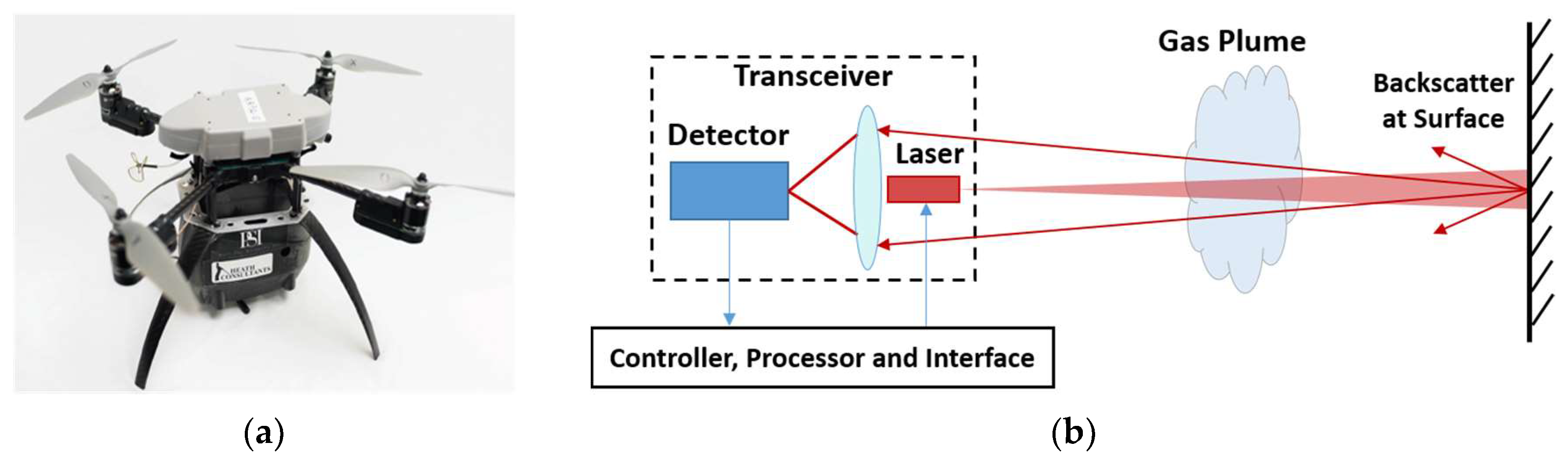
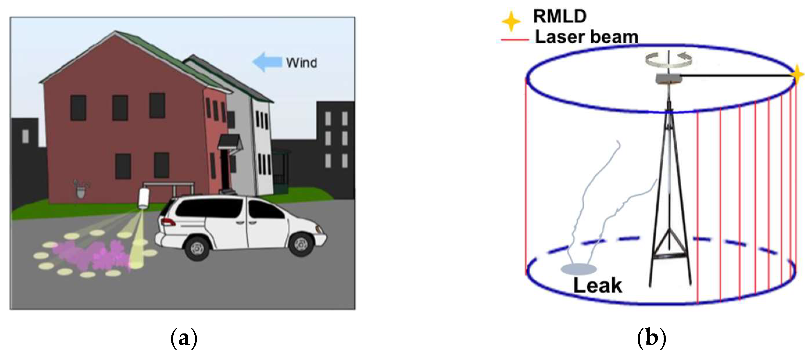
4 laser sensors, a custom small UAV, which is shown in Figure 1a, Global Positioning System (GPS) navigation, a semi-autonomous control unit and data acquisition and processing software. Table 1 shows the specifications of the RMLD-UAV system.
The RMLD-UAV system is centered on the RMLD technology, which is widely deployed worldwide for natural gas leak surveying. This eye-safe laser-based CH4 detector that surveys natural gas infrastructure complies with EN 60825-1 MPE for an eye-safe Class 1 laser at 1650 nm with a 0.01-W output. RMLD detects CH4 with 5-ppm-m sensitivity at a distance from 0–15 m compared with the 200-ppm-m sensitivity of the Pergam Laser Methane Copter (LMC) [56]. The basic RMLD operating principle is shown in Figure 1b [57,58]: An infrared laser beam exits a transceiver unit and is projected to a surface. A fraction of the beam is scattered from the surface and is captured and focused onto a photodetector. The received laser power is converted to an electronic signal. The wet mixing ratio of CH
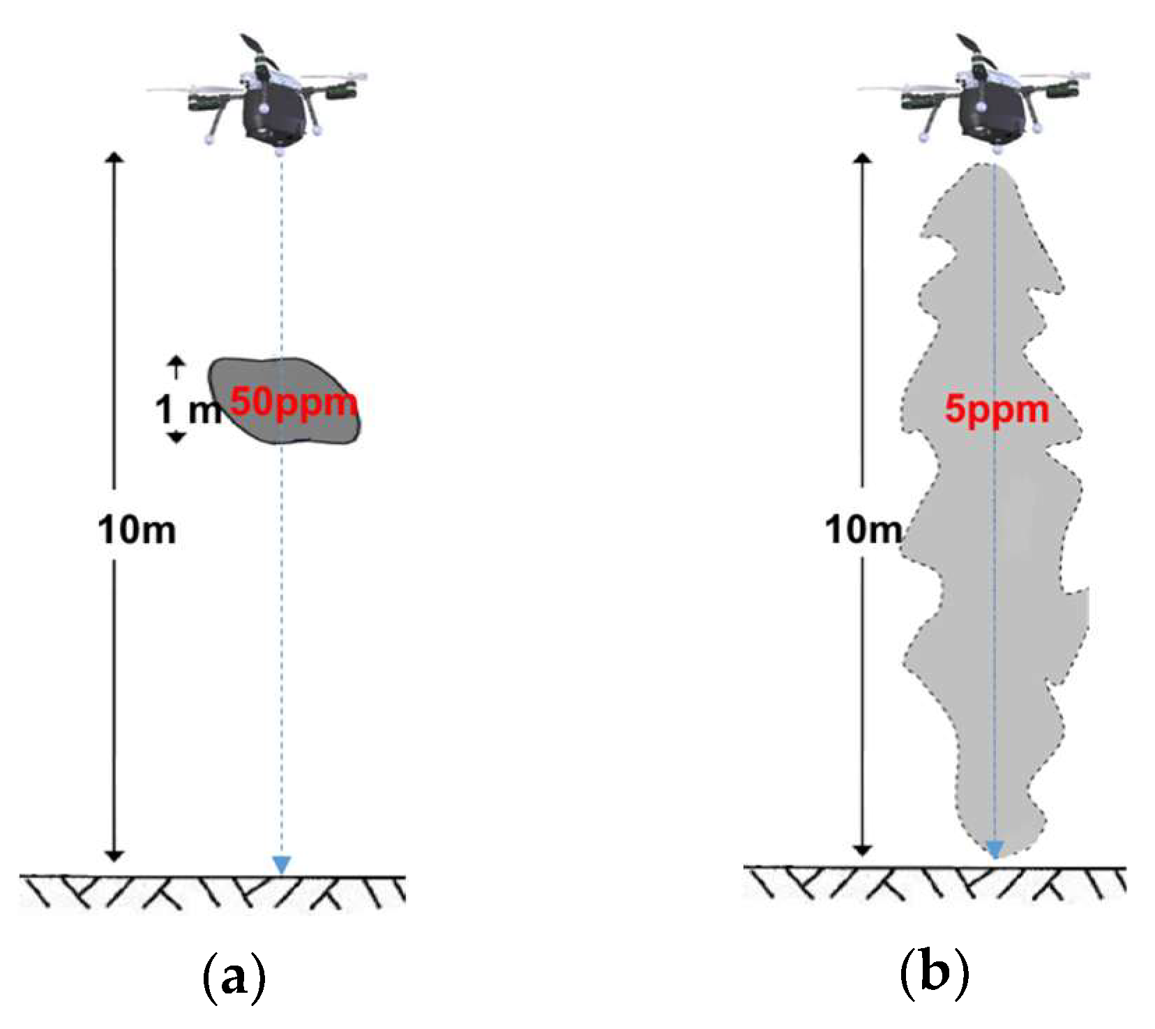
4 is obtained by processing received signals. Scanning the laser beam across gas plumes results in rapid gas analysis. The laser beam width is 1 cm at the transceiver and about 15 cm at 10 m. Operating as an open path sensor, the RMLD-UAV laser beam aims at the ground from the UAV and measures column-integrated wet CH4 mixing ratios that average the variations in the vertical CH4 distribution, as shown in Figure 2. The temperature and pressure over the laser path are assumed constant due to the low survey altitude (<10 m). The CH4 readings are reported in parts per million meters (ppm-m).
The system calibration includes two parts, zero calibration and span calibration, which are the common routines in gas analyzers. The zero point is measured with the laser projected over a short path length (~1 m). Span is measured by projecting the laser through a sealed glass cell containing the equivalent of 900 ppm-m CH4. The slope of the line connecting the two points is the calibration constant that converts measured raw signals to ppm-m. The calibration is conducted when the sampling site is changed or under some other circumstances, which may result in the change of general sampling elevation or meteorological conditions.
Sensor technology is a limitation for the use of small lightweight UAVs. Until recently, there were few high precision CH4 instruments suitable for such a platform. Backscatter Tunable Diode Laser Absorption Spectroscopy (TDLAS) is the main technology of the RMLD to deduce column-integrated CH4 mixing ratios over the straight laser path. The measurement principle is absorption spectroscopy. Most simple gas-phase molecules have a near-infrared to mid-infrared absorption spectrum, which consists of a series of narrow, well-resolved, lines, each at a characteristic wavelength. Because these “absorption lines” are well spaced and their wavelengths are well known, the mixing ratio of any species can be determined by measuring the magnitude of this absorption as a laser beam passes through a gas cloud. In the TDLAS system, a diode laser emits light at a well-defined, but tunable wavelength corresponding to a specific absorption line of the target gas, which is free of the spectral interferences from ambient gases. TDLAS has low cross-sensitivity and is able to detect single gases [59]. The wavelength centers on 1.6 µm when CH4 is the targeted gas and other gases in the ambient air are invisible. Active TDLAS sensor has several attractive features, such as reliable laser sources, low power consumption (<1 W), ambient temperature resistance (−20 °C~50 °C), highly compact, continuously operating, minimal maintenance and acceptable cost [60]. There are also some adverse conditions that may affect the leak detection, such as precipitation or other obstructions in the line of the targeted sources.
The laser’s fast tuning capability is exploited by the sensor to rapidly modulate the wavelength. The response to the wavelength modulation is an amplitude modulation at the detector. The amplitude modulation arises from two sources: (1) the transmitted laser power sinusoidally modulating at frequency ωm and (2) the absorption due to target gas occurring at precisely twice the modulation frequency 2ωm since the target gas absorption line is swept twice in each modulation cycle. The average values of the amplitude modulations at ωm and 2ωm are analyzed by the signal processor, which are Signals 1 and 2, respectively. Signal 1 (F1) is proportional to the received laser power, while Signal 2 (F2) is proportional to the combination of the received laser power and the path-integrated concentrations of the target gas. Therefore, the ratio F2 over F1 can be taken to reflect the analyte abundance, which is independent of the received laser power [61]. This feature enables the sensor to properly track mixing ratios despite changes in laser power transmitted across the optical path. The laser power change can appear, for instance, due to the variability in reflectance of illuminated backscatter surfaces or dust in the optical path. This feature is critical in RMLD-UAV applications since the reflectance of the targeted surface from which the backscatter signal is received changes continually in a mobile system. The phase demodulation and lock-in amplification technique in the RMLD is called Wavelength Modulation Spectroscopy (WMS). The laser is initially “tuned” to the center of the absorption line via temperature. The laser wavelength is then scanned repeatedly across a portion of the spectral absorption line via its injection current, thus producing an amplitude-modulated signal of the laser power received at the detector. Radio receiver technology is used to process or demodulate the small signal to yield an output indicating a molecular concentration in target gas. WMS measures the absorbance of 10−5 or less with 1 s or faster response and has a highly sensitive and fast capability to realize spectroscopic gas analysis. It can provide a sub-ppm chemical detection limit with sub-second or faster response time.
There are several limitations that constrain the application of the UAV system. Small UAVs are subject to significant payload restrictions, short flight endurance, network communication limits and FAA flight restrictions compared to larger manned aircraft. Despite these limitations, small UAVs have distinct advantages over their manned counterparts in terms of relatively low platform cost, operation flexibility and capability to perform autonomous flight operations from take-off to landing. The UAV we used is a customized rotary wing drone with the electric quadcopter motor model propulsion system, MT 2216-9 KV 1100. This miniaturized UAV has a relatively low operating speed, but it allows hovering status for close proximity inspection. The composition of the UAV includes plastic, carbon composite and aluminum frame elements and electronic circuit boards. The UAV is equipped with a small size, lightweight visible-spectrum camera (NTSC RS-170, 5.8-GHz analog transmission), providing a view of the area interrogated by the laser.
The commercial RMLD product is a two-component device comprising a 2.7-kg control unit carried by a shoulder strap attached by an umbilical cable to a 1.4-kg handheld transceiver. Traditional RMLD’s portable, battery-powered configuration is designed and developed for walking investigations, which simplifies the work of surveyors compared to the traditional flame ionization detectors. Traditional RMLD is a manually-operated gas analyzer without a positioning system and can only detect the gas leak and measure the gas path-integrated mixing ratio in ppm-m without locating the leak position. In order to develop the sensor to be mounted onboard a UAV and match the current capabilities of the UAV while maintaining CH4 detection sensitivity, the decade-old technology has been improved and the sensor has been scaled down to an appropriate Size, Weight and Power (SWaP) with respect to the manageable payload. Some technical developments have been achieved to realize the miniature integrated devices serving the RMLD-UAV, such as opto-mechanical design, detailed electronics design, power consumption, integrated circuit electronics and wireless transmitters. Specifically, the original near-IR Distributed Feedback (DFB) laser was replaced by a 3.34-µm DFB-Interband Cascade Laser (ICL); the transceiver size was reduced while still allowing flight up to a 10-m altitude; the circuit board was reduced to 77 cm2 from the previous 232 cm2 to fit the miniature UAV footprint; and a 2.4-GHz encrypted radio link for wireless data exchange with the ground control station was added. Mini-RMLD is a single compact unit weighing approximately 0.45 kg and shares its battery with the UAV. It includes GPS and Bluetooth, which can realize real-time data acquisition and transmission. Coupled with the preprogrammed quantification and localization software, the semi-autonomous RMLD-UAV system can provide estimations of leak rate and source location, as will be described in the following sections.

2.2. System Operation and Data Acquisition

As a semi-autonomous system, on the one hand, a pilot initiates the launch of the UAV and controls the recovery via the UAV-side mission controller. On the other hand, the drone can be flown autonomously with preprogrammed electronic flight plans using the laptop-based custom Ground Control Station (GCS).
The mission controller displays the flight information and status derived from flight instrumentation. The UAV can be navigated visually using the controller unit and return to taking-off and landing automatically. Recent advances in control have made unstable platforms such as small UAVs more reliable and easier to operate, reducing the risk of payload damage and accidents in general. RMLD-UAV has a redundant system, and emergency procedure commands are immediately available to the UAV pilot. The pilot can take control at any time and manually pilot the UAV. Alternatively, the UAV pilot can also select the “Return to Home” function on the remote, and the UAV will return to its starting position. A built-in GPS supplies position information that is used by the UAV system to realize waypoint navigation, as well as to synchronize the RMLD data. The waypoints describe the three-Dimensional (3D) location of the drone at that point in the flight path, with a latitude, longitude and altitude. In the field tests, the intended survey altitude is around 10 m, at which height the signal of the background level CH4 is relatively stable and low, and RMLD-UAV endeavored to maintain at the steady flight height during a sampling mission in order to subtract the background column and offset the influence of the ambient signal. The influence of the background CH4 signal increases notably with flight altitude above 10 m, which will be discussed in detail in Section 3. Flight plan updates can be issued while in flight. The mission controller handles the receipt of target waypoints and emits telemetry and mission status packets to the GCS.
The GCS is full-featured for the autopilot platform with a custom mission planner software. It provides an intuitive and simple Graphical User Interface (GUI) and Google Maps Application Program Interface (API) with which waypoint missions can be defined and autonomous flight paths can be planned, saved and uploaded into the UAV. In addition, this GCS is deployed with software that can process the collected data and analyze the leak rate and leak location in several seconds. In the future, the system will continually and autonomously monitor targeted sources via the combination of two approaches: fence area monitoring and daily routine detection.
However, the RMLD sensor cannot directly supply the information of source location and the leak rate of gas emissions. Leak localization and quantification procedures and algorithms are required. The RMLD-UAV system acquires data during a 15–20-min flight mission, and then, the measurements are processed in near-real-time (several minutes within landing) by leak localization and quantification algorithms to provide estimations.

2.3. Quantification Algorithm

Besides the RMLD-UAV technologies, an accurate quantification algorithm is also a crucial factor to estimate the leak rates and guide the further investigation. The mass flux is broadly defined as the flow rate of a species per unit area of a defined cross-sectional plane downwind of the source. For most atmospheric calculation cases, the spatial gas density and wind are not homogeneous within a source domain. Thus, the standard calculus approach needs to be applied to solve problems by dividing the cross-surface into pieces, finding the flux at each segmented surface and integrating the small units to get the total flow rate. Therefore, in the mass balance approach, the flow rate (q) of gas through a vertical plane downwind of a source domain is estimated as [62]:
q = 0 H W / 2 W / 2 u × ( X X b ) d x   d z
where H and W are the vertical and lateral dimensions of the gas plume, u is the wind component perpendicular to the plane and ( X X b ) is the enhancement of the gas mixing ratio above the background, and the full integration over the limits of the plane yields an emission rate. In the current RMLD-UAV sampling system, the horizontal wind is measured at one fixed location supplying an approximate uniform wind speed to each segment. The direction of the wind component of each segment can be obtained according to the angle between the mean wind direction and the orientation of the vertical plane deriving from the laser track.
In the common analytical and numerical quantification approaches, the atmospheric transport model needs to be implemented due to the distance away from the source, and the background gas concentration needs to be known. In the aircraft-based mass balance approach, the measurements of the point gas analyzer (e.g., CRDS) at multiple altitudes need to be integrated. As an open path monitor, RMLD-UAV measures the vertical total amount of a specific gas parcel in the path of the laser beam, indicated as 0 H X   d z in ppm-m. Besides, the RMLD-UAV system can be close to the leak source (several meters), eliminating the atmospheric dispersion and buoyancy effects. Typically, a fugitive plume emitted from a point source travels in the direction of the mean wind and disperses vertically and horizontally due to the mixing of turbulent eddies. Furthermore, the sampling system is designed to scan a surface that encloses the leak source, creating an arbitrarily-shaped laser curtain (e.g., cylinder). By convention, positive flux leaves a closed area, and negative flux enters a closed area. Therefore, the upwind gas plume entering the laser path yields negative flux, and the downwind plume leaving the laser curtain yields positive flux. During the computational process, the positive or negative flux is determined along with the geometry operation. Combining the mass conservation principle, the integration of all the positive fluxes and negative fluxes can counteract the influence of the ambient CH4 signal, and only CH
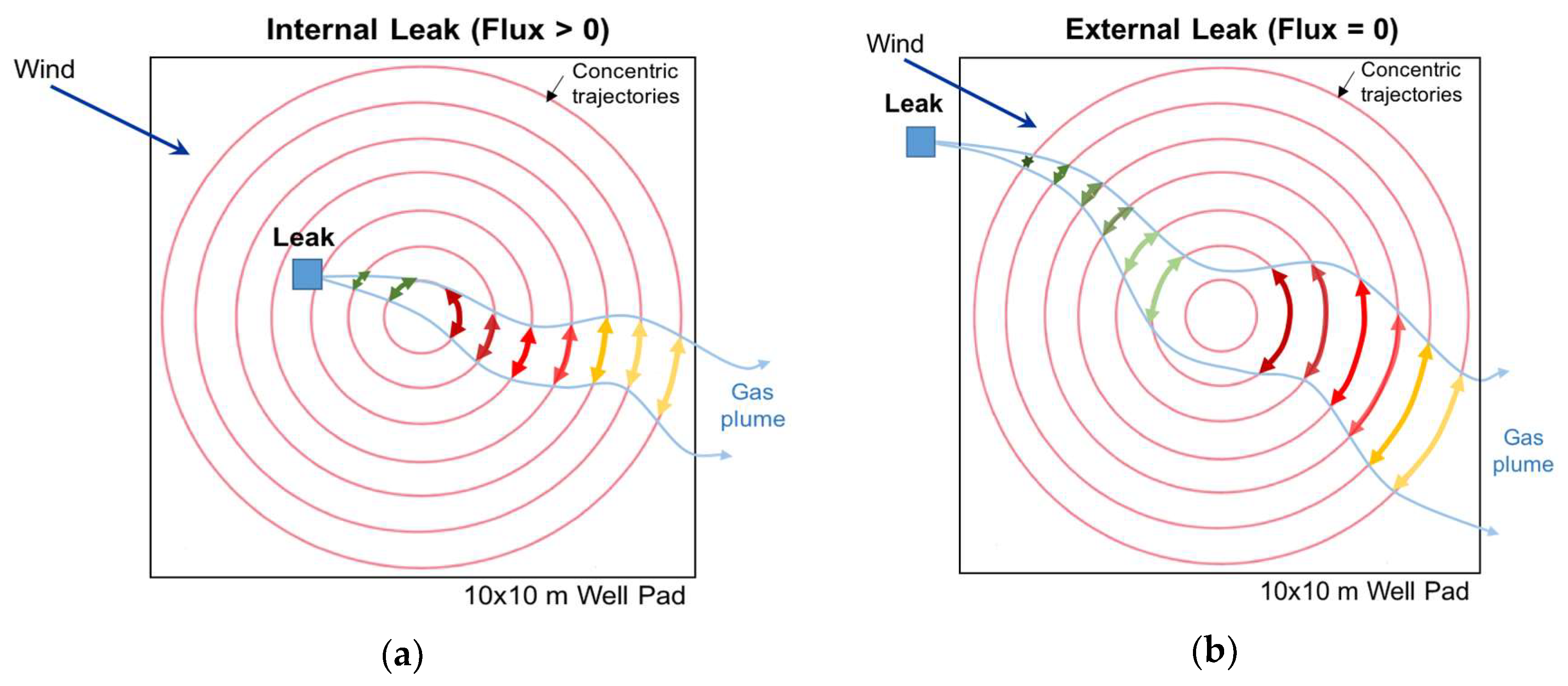
4 emitted from within the enclosed area yields a non-zero net flux. An imbalance between the positive and negative fluxes indicates the existence of a leak. Furthermore, due to the mass balance, fluxes of a series of concentric shapes that encircle the leak source should yield the same leak rate results. The error contributions of unsteady winds on the leak rate estimations can be diminished by averaging the multiple results from each cycle. Figure 3 shows the two sampling examples of the internal leak source and external leak source of a well pad. Multiple concentric trajectories were conducted within the well pad area. By integrating the negative fluxes (greenish arcs) and positive fluxes (reddish arcs) of each circle and averaging the net flux of each circle, the leak rate ( Q ) of the targeted source can be estimated as:
  Q = i = 1 n q i n  
where 
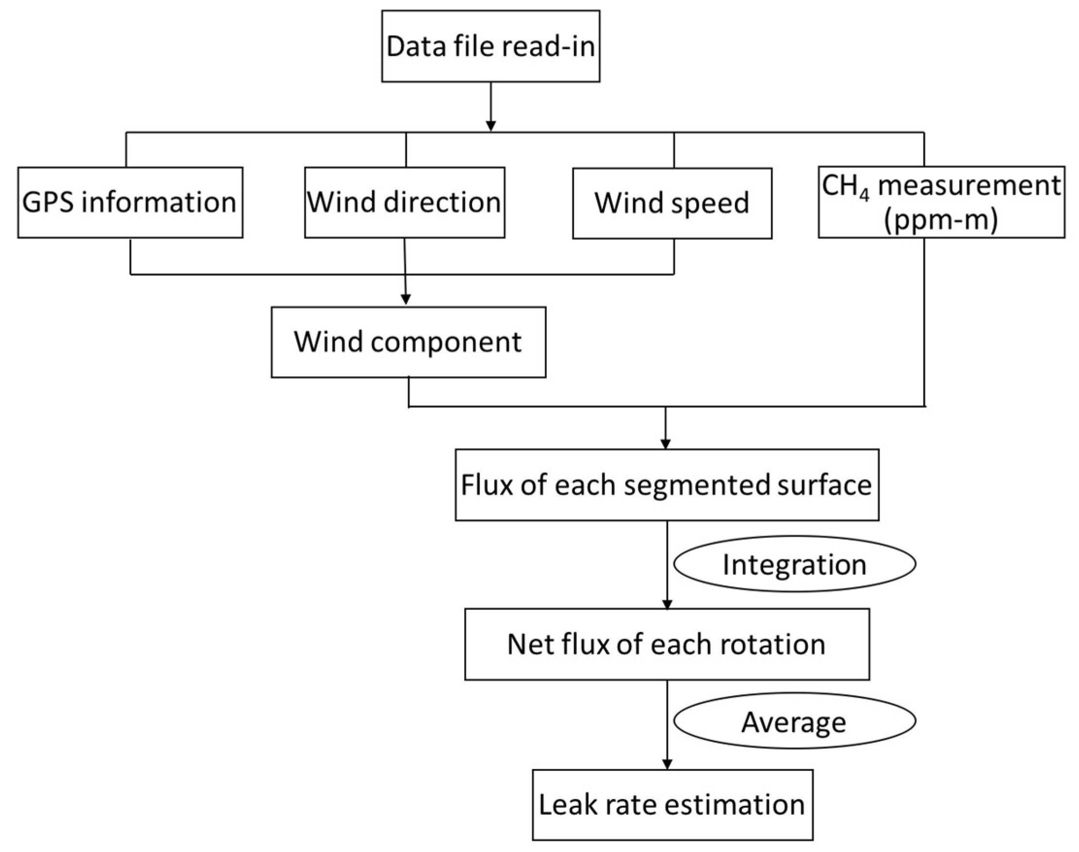
n is the number of shapes that enclose the leak and q is the total flux of each enclosed path. The flowchart of the basic calculation algorithm is shown in Figure 4.

3. Sampling Strategy Attempts and Quantification Results

We conducted several field tests and iterated through several stages of sampling strategies depending on the development progress of the system since May 2015. A series of field tests was conducted at five test sites: (1) New Jersey site, PSE&G Edison Training facility; (2) Texas Site 1, Blimp Base Interests in Hitchcock; (3) Plaistow site in New Hampshire; (4) Texas Site 2, Heath consultants /Physical Sciences Inc. validation platform site in Houston; (5) Colorado site, Methane Emission Technology Evaluation Center (METEC). At the New Jersey site, Plaistow site and Texas sites, controlled emissions were from 99.5% pure CH4 and metered by a Dwyer RMB-52 flowmeter. A specific gravity correction factor was used since the meter was calibrated for air. The correction factor equation is:
Q 2 = Q 1 × 1 / S . G .
where Q 2 is the standard flow rate, Q 1 is the observed reading of flow rate and S . G . is the specific gravity of CH4, which is 0.5537. At the Colorado METEC site, the release was pipeline gas, and flow rates were controlled by orifices.
In the early stages, several trials were designed and implemented to test the feasibility of the first-generation mini-RMLD to evaluate the performance of the calculation algorithm. These introductory tests were conducted at the New Jersey site and Texas Site 1 during May 2015–May 2016. In these trials, the RMLD or mini-RMLD was fixed on two rotating devices aiming down to the ground below. The conceptual sketch of both example systems is shown in Figure 5. The average wind speed was obtained from a local anemometer. These preliminary tests have led to multiple combinations of sampling strategies and flux calculation algorithms and provided valuable lessons. It was found that the signal of elevated CH4 was more obvious in the larger leaks, and the influence of background noise was more crucial in small leak cases. Besides, the largest errors were associated with extremely small leak rates. Furthermore, multiple rotations improved final leak rate estimation under the steady wind conditions. The initial measurements validated the performance of the quantification algorithm and the practicability of using mini-RMLD in a rotating system.
After verifying the capability of traditional RMLD and mini-RMLD using several rotating devices, the RMLD-UAV system was integrated, and the semi-autonomous system has been available for measuring CH4 leaks since June 2016. 
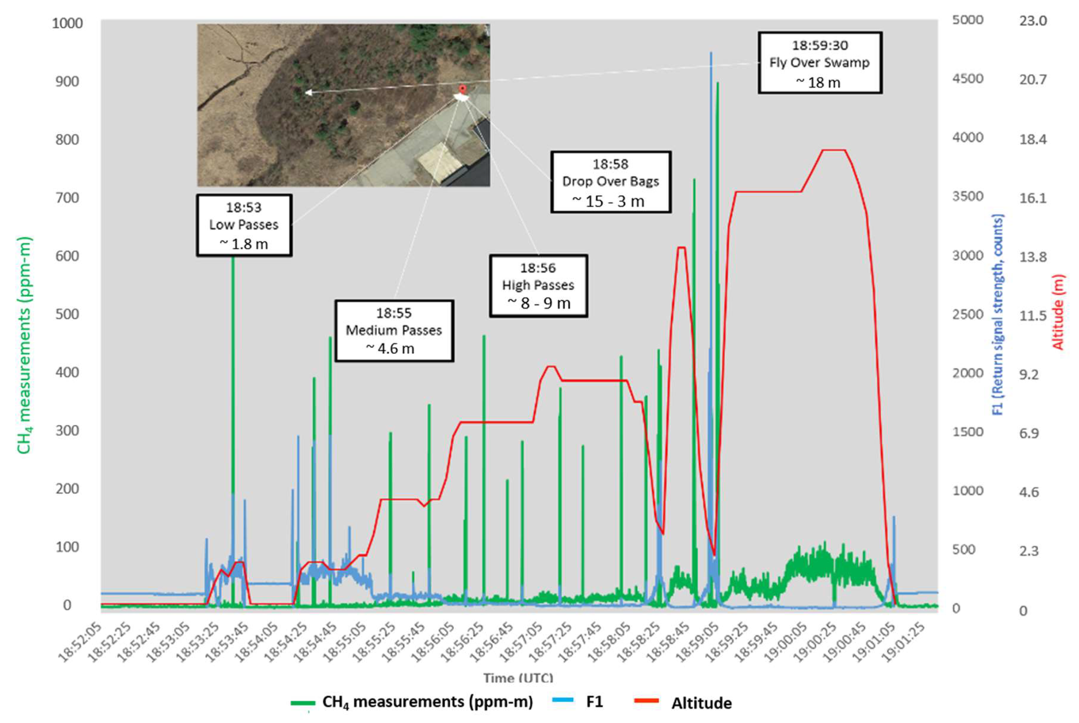
Figure 6 shows the first test flight conducted in Plaistow, New Hampshire. Several transparent CH4-filled plastic bags (30 cm × 30 cm, 100% CH4 with a thickness of about 1 cm) were fixed on the ground as the simulated leak sources. Viewed from the on-board camera with superimposed flight data, it was demonstrated that each pass over a leak source yielded a large CH4 measurement spike. At low altitudes, passes over bags also increased F1 signals due to the increased reflectance of the bag surface. From 18:59:05–19:01:25, the RMLD-UAV flew over a swamp showing the largest background level CH4 signals due to both swamp gas CH4 and noise of rather low laser power (low F1). In this test, multiple passes at various heights over source bags illustrated the detecting capability of the RMLD-UAV system. CH4 and F1 signals vs. height demonstrated the operating range and sensitivity of the system. One thing noted was that, under the designed survey altitude (<10 m), the detected background CH4 signal by RMLD-UAV maintained at a steady lower level; whereas the background level path-integrated CH4 mixing ratio increased markedly with a flight altitude above 10 m. Compared with the signal of the simulated CH4 sources with extremely high concentration, the background path-integrated CH4 mixing ratios seemed too high (the green line of the CH4 signal was noisier and as high as around 100 ppm-m at an 18-m height). By checking the raw signals of the mini-RMLD, an increase of mini-RMLD noise with the movement was discovered. The noise source was traced to an optical component that failed to meet specifications. The situation of excess noise was improved for the next-generation mini-RMLD in the following field tests.
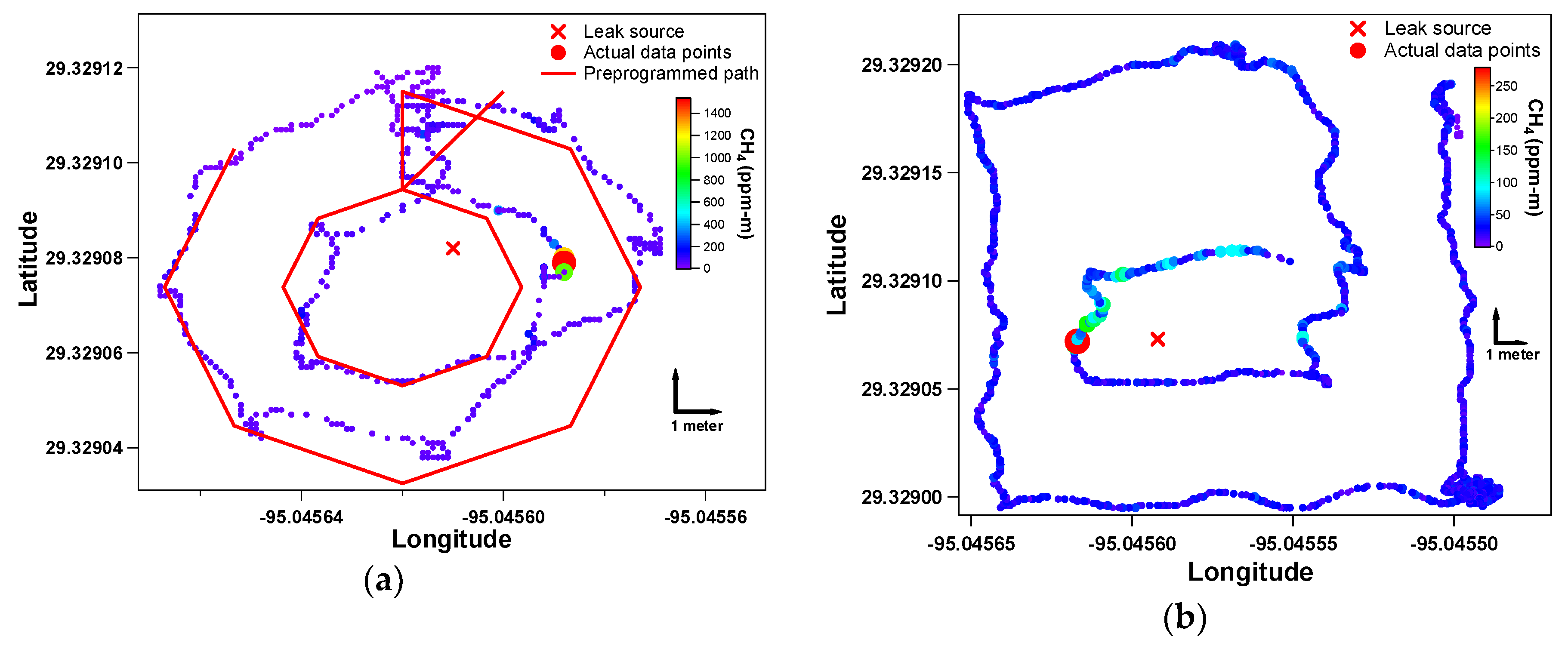
Some follow-up flight tests were deployed at Texas Site 1 to estimate the system performance and to find the optimal flight pattern. The simulated leak point was set manually in the field. Due to the restrictions of system manipulation (waypoint navigation) and data acquisition needs, some regular geometric sampling shapes with relatively few waypoints were tested. The flight height was around 5–10 m. The particular flight patterns were preprogrammed, and the synchronized GPS data indicated the exact data points and flight path of the RMLD-UAV. Flight cases of a series of boxes and octagons are illustrated in Figure 7, with controlled CH4 flow rates of 1.59   × 10 4 standard cubic meters per second (m3/s) and 2.12   × 10 4 m3/s, respectively. The calculated leak rate was 2.33   × 10 4 m3/s in the octagon case, and the estimation of box case was 3.22   × 10 4 m3/s. It is easy to observe that the actual flight path did not perfectly follow the preprogrammed path. In addition, there were roving behaviors near waypoints in both flight patterns. The vehicle maneuvered typically up to several minutes until it was within 1 m of a particular waypoint. The redundancy of data points near waypoints added error to the result estimation due to the error in the surface integral calculation. This indicated that an alternative flight pattern was needed to overcome the imperfect sampling system and to improve the accuracy of the quantification results.
From March–July 2017, multiple further field tests were conducted at two Texas sites (Site 1 and Site 2) and the Colorado METEC site to optimize the flight strategy and evaluate the system performance when surveying simulated natural gas infrastructure. RMLD-UAV flew at the maximum design altitude (10 m). The anemometer was set near the sites. Table 2 shows the specific deployment information for each test.
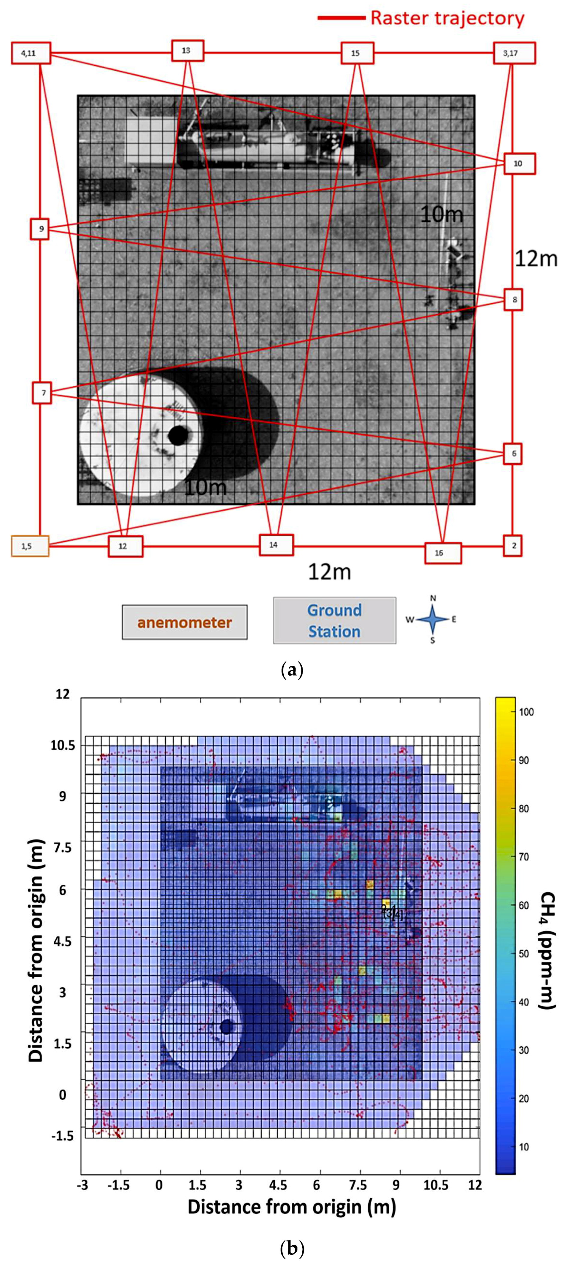
Several months of testing led to various flight track attempts and different iterations of flux algorithms. Flight pattern and sampling strategies investigated included series of boxes (a series of concentric squares of flight path formed around the leak source), downwind screen (a sampling conducted in the downwind of the leak source), random full coverage (a random flight covering the whole test field), zigzag (a jagged flight pattern, which is made up of small corners at variable angles between the field boundaries), perimeter zigzag (a zigzag flight pattern plus a perimeter sampling around the field boundary), roving near leaks, random hovering and raster scan (a pattern in which the flight path sweeps horizontally left-to-right and then retraces vertically up-to-down). Some lessons can be learned from the flights and data: simple flight patterns (e.g., series of boxes) were irregular and imprecise under unsteady wind conditions; more data, especially near the leak source, were better to enable an averaging process and convergence to an acceptable accuracy upon collecting sufficient statistics. Based on these tests, the raster-scan flight track, which covered the whole test field, was found to be the optimal strategy for operating the system and quantifying the emission leak rate, as shown in 
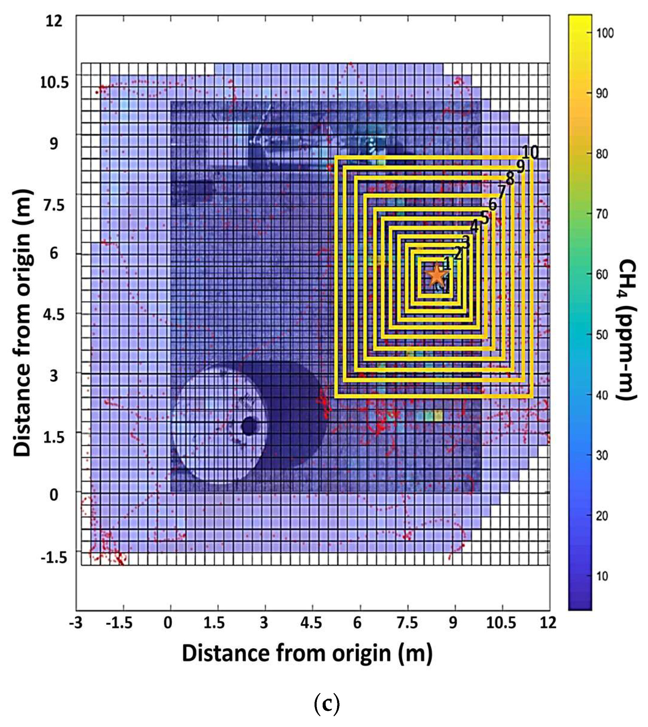
Figure 8a. The field needed to be fully scanned, and no specific flight pattern was required, which was easier to implement. After executing a coarse scan of the test field, measurements from RMLD-UAV were processed via a MATLAB routine. The inputs included CH4 measurements, wind information and 3D (latitude, longitude and altitude) locations of each data point. The program output an array of uniformly-spaced pixels with interpolated values from the original randomly-spaced data points. The interpolation method we used was the triangulation-based natural neighbor interpolation, which was an efficient tradeoff between linear and cubic. The generated interpolated heat map is shown in Figure 8b. By conducting several tests, the leak localization method based on finding maximum CH4 measurement pixel was proven to have the most reliable performance [55]. Thus, the max-CH4 measurement pixel was considered as the leak source position. In Figure 8c, multiple concentric boxes are traced and developed around the max-CH4 pixel center to calculate the leak rate. The averaged wind speed and wind direction during one particular case period were used to eliminate the influence of wind variation. The final leak rate estimation was calculated by averaging the total flux of 10 boxes in this case.
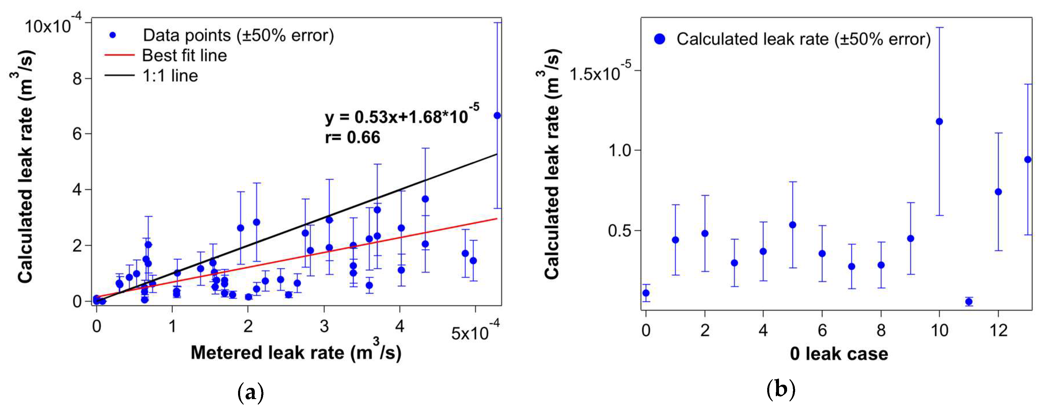
The performance of this approach is illustrated in Figure 9. The estimations were obtained from all the datasets shown in Table 2. It can be ascertained that this mass balance-based algorithm on average tended to underestimate leak rate, as shown in 
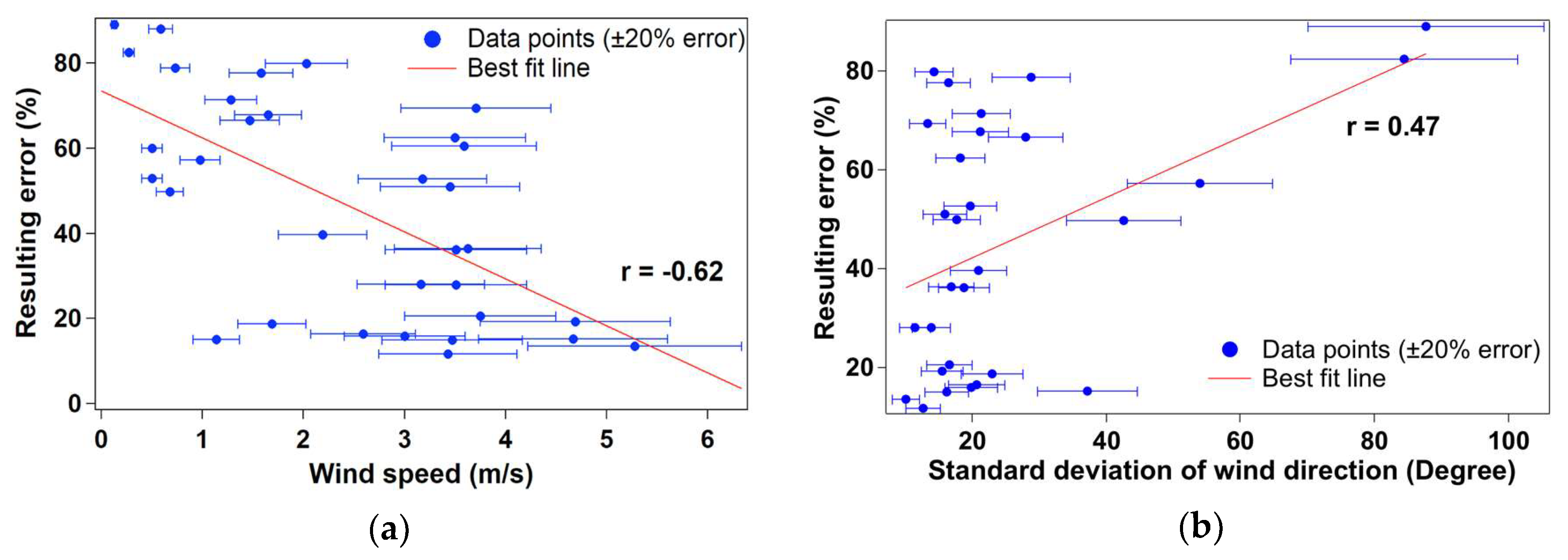
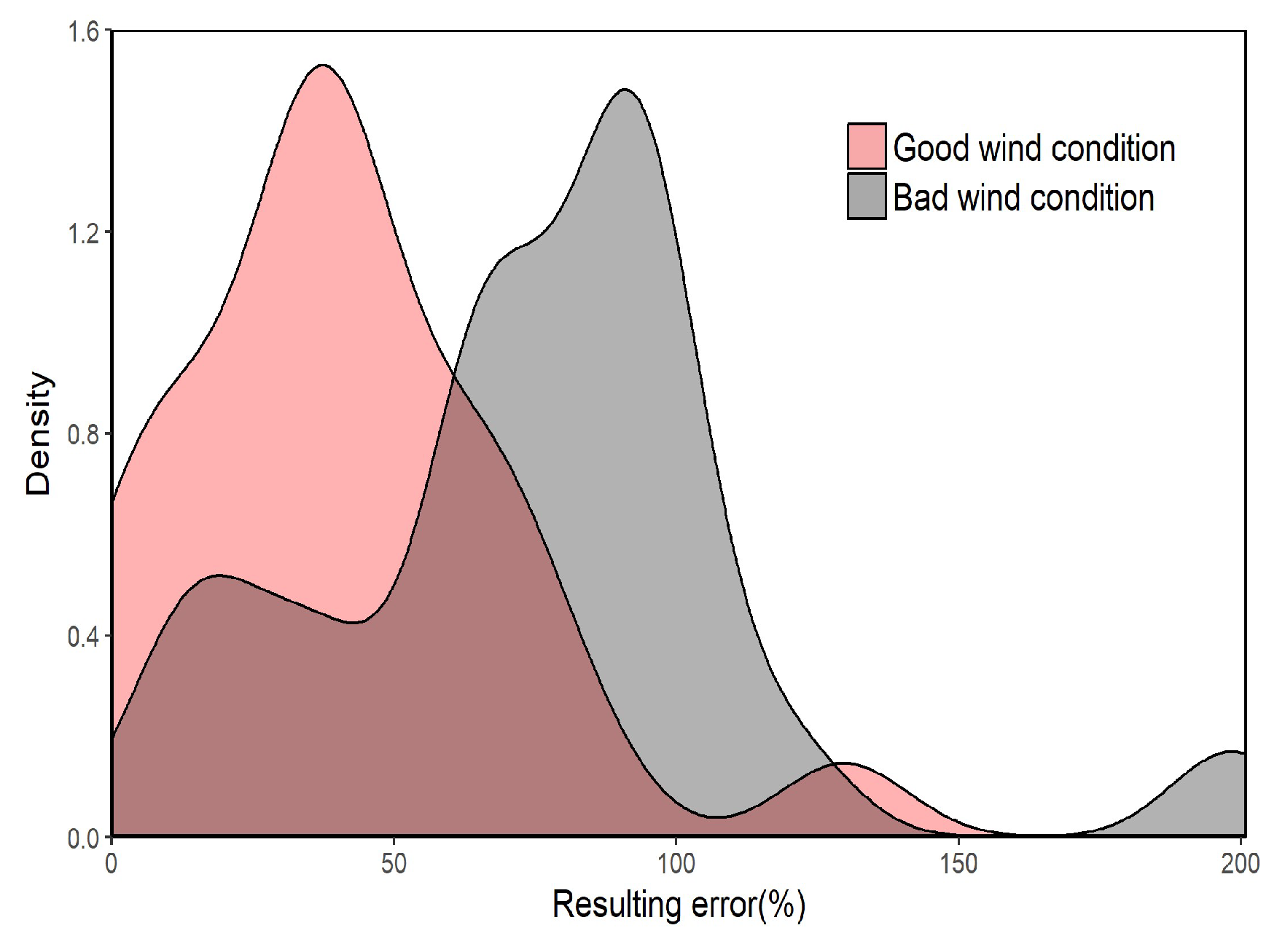
Figure 9a. Theoretically, only the max-CH4 data point located near the center of the interpolated map could generate multiple boxes and could ideally supply a good estimation by averaging the results of multiple boxes. A secondary finer scan around the possible source was needed to deal with the limitation of this approach. It is significant to remind that wind condition was crucial to the leak rate estimation. Further analysis of the results and method accuracy considering different wind conditions are discussed in the next section. This preliminary algorithm was encouraging, but not optimal. A refined algorithm needed to be developed to improve the quantification method upon the mass balance algorithm. The further development and the investigation of several alternative algorithms are described in the companion paper of this work [55].
In order to calibrate the system and evaluate the performance of the quantification algorithm, several zero leak tests were also conducted. The calculated leak rates are shown in Figure 9b. The mass balance quantification algorithm yielded very small numbers of leak rate for the zero-leak cases (less than 1   × 10 5 m3/s); however, some of the positive leak cases also had estimates below 1   × 10 5 m3/s. The zero-leak cases were difficult to determine exactly using the quantification algorithm alone due to the systematic errors, the noise of the mini-RMLD, the numerical principle of the algorithm and variable atmospheric conditions. In addition, the experience of previous field test pointed out that the mini-RMLD had unreliable performance in detecting leaks under 7   × 10 6 m3/s (~1 Standard Cubic Feet per Hour (SCFH)). Taken all together, the zero leak cases were hard to clarify. Other parameters that could constrain the zero-leak calculation needed to be considered. As a proposed indicator, skewness was introduced and is discussed in detail in next section.

4. Uncertainty Analysis and Zero-Leak Investigation

4.1. Uncertainty Analysis

According to the quantification algorithm, there are three key quantities that influence the final estimations: wind information from the in situ weather station, CH4 measurements from RMLD and data position from GPS. It is important to understand the effect of different ambient circumstances and the possible errors of particular measurements may have on emission estimations. As an ongoing project, the instrumentations keep being improved and updated. In order to evaluate the influence of these quantities and their associated uncertainties, the influence of wind condition was analyzed, and random noise was added to the mixing ratio measurements and GPS position measurements.
The system performance under different wind conditions was analyzed to understand the influence of wind and to find the optimal operating protocol. As a vector quantity, there are two aspects of wind that need to be considered, wind speed and wind direction. From the intuition of gas plume dispersion, the magnitude of wind speed and the variation of wind direction are two major factors influencing the leak rate estimation. The leak rate resulting errors versus Wind Speed (WS) and Standard Deviation of Wind Direction (STDV_WD) are plotted in Figure 10. Each corresponding WS is the average value calculated from the ground-station measurements during each sampling (15–20 min), and the STDV_WD is also obtained within each sampling duration. It turns out that there is a negative correlation (r = −0.62) between the resulting error and WS, while the correlation between the resulting error and the STDV_WD is moderate positive (r = 0.47). This partly confirms the intuitive expectation that higher WS and steadier WD can lead to lower errors and better leak rate estimations. The results suggest that wind speed plays a larger role in the quality control of the leak rate estimations regarding wind conditions. It is also important to note that the cases with the extremely variable wind directions (STDV_WD > 40 degree) have larger resultant errors and have a major influence on the stated positive correlation. The calculated p-value was 3% (<5%) indicating a statistically-significant result.
Given the dependence on wind conditions found, the results of Figure 9 were interpreted separately under preferred or bad wind conditions, as shown in Figure 11. The wind information of all the field tests was investigated, and two criteria regarding WS and STDV_WD were determined to define good or bad wind conditions. Two-point-three meters per second and 33.1 degrees are the thresholds of WS and STDV_WD, respectively. A good wind condition is defined to have both a WS that is larger than 2.3 m/s and steady WD, of which STDV_WD is smaller than 33.1 degrees, whereas a bad wind condition does not meet one or both of the criteria. About half of the tests (24) had good wind conditions, and 23 cases were under a bad wind condition. It can be seen that performance of the method has approximately 50% accuracy (highest density) in good wind cases, and the accuracy in bad wind cases is around 100%, excluding some outliers.
The influence of raw CH4 measurement errors on the leak rate calculation needs to be clarified. The effect of the atmospheric turbulence on RMLD-UAV can lead to GPS measurements errors, which also need to be considered and investigated. A random number that followed the uniform probability distribution was generated and added to each raw measurement. Specifically, 20% and 50% random noise were added to the original CH4 measurement, respectively, to simulate the sensor uncertainty. One-meter and 2-m noise were added to the latitude and longitude data to consider the GPS uncertainty. The newly calculated leak rate is compared with the original results to investigate the influence of the added noise on the calculated leak rates. The leak rate deviation from the original (relative leak rate error) is shown in Figure 12. The leak rate errors distributed within ±10% after adding 20% noise to the mixing ratio measurements, and the errors distributed within ±25% after adding 50% mixing ratio noise. These results are foregone conclusions in the sense that leak rate is linearly related to CH4 measurements in the quantification algorithm. On the other hand, we can see that the leak rate error increases with GPS noise. One-meter noise yields both positive and negative errors in the leak rate estimations and generally results in errors within ±40%; while 2-m noise tends to yield positive errors on leak rate estimations, which is due to a larger cross-section at a larger distance from the source.

4.2. Identification of Zero-Leak Cases

In order to clarify the zero-leak estimations, the raw CH4 measurements are analyzed. Figure 13 shows the example CH4 measurements’ probability distribution. The measurements are filtered, and only the data collected during flight are considered. It can be seen that zero-leak case has a near normal Gaussian distribution in the lower CH4 values, which indicates the signal from only background CH4. The signals are generally less than 20 ppm-m. In comparison, the non-zero-leak case has a skewed distribution with a long tail on the right. The left clustered CH4 signal is from the background, and the signal of the long tail is from the elevated CH4 leaks.
From the effect on the CH4 distribution, we introduced skewness as an indicator to clarify zero-leak cases. Skewness is a moment coefficient indicating the degree of asymmetry of the distribution about the mean, defined as:
s = i = 1 N ( x i μ ) 3 / N σ 3 ,
where N is the number of data points, x i is an individual CH4 measurement of RMLD-UAV, μ is the mean of x and σ is the standard deviation of x . The skewness of all the testing cases was calculated, and the correlation between metered leak rates and skewness was analyzed to find the characteristic of zero-leak cases in Figure 14. The correlation coefficient is 0.79, which means that larger leaks tend to have larger skewness. If we calculate the skewness of all the zero-leak cases, it is easy to find that all the zero-leak cases have skewness values less than 0.5, and all of the positive leak cases have a skewness value above 0.5. Thus, the parameter of skewness is treated as a distinct zero-leak indicator, and 0.5 is taken as the empirical threshold to clarify the zero-leak cases at this stage.

5. Conclusions and Implications

RMLD-UAV is proven to have a reliable ability for monitoring fugitive CH4 leak rate through a detailed suite of field tests. The configuration of the system can realize semi-autonomous surveying missions, immediate data acquisition and visualization and near real-time localization and quantification reporting. Several months of field testing contributed to optimizing the sampling flight strategy and led to different iterations of flux algorithms. The mass balance flux calculation algorithm incorporating a raster-scan flight pattern and interpolated concentration map tended to underestimate the flow rates, and the detection limit of this method was around 7   × 10 6 m3/s (~1 Standard Cubic Feet per Hour (SCFH)). The wind condition plays a significant role in this method, and the performance of the method is evaluated separately under good or bad wind conditions. Higher wind speed and steadier winds are preferred to get better results. The accuracy of the method is about 50% under preferred wind conditions (with higher wind speed and steadier wind direction) and distributes around 100% under bad wind circumstances. Since a key motivation for characterizing flux is to prioritize repairs, this magnitude of error is acceptable for practical use where real-world leak rates may range over several orders of magnitude. The skewness is a promising indicator to clarify the zero-leak cases and positive leak cases. The influences of some key parameters on the accuracy of the quantification results are different. We found that GPS noise has the greatest impact on the leak rate estimations. The up to 2-m noise of position measurements can add more than 100% error to the leak rate results. However, the GPS device should have less than 1-m noise with the RMLD-UAV system. In summary, better leak rate estimation requires high precision latitude and longitude data from the GPS; accurate wind measurements and favorable wind conditions; an appropriate flight pattern and a relative steady flight height (~10 m) of the drone.
The RMLD-UAV system has advanced leak detection capabilities for monitoring and quantifying CH4 fugitive leaks from the natural gas industry. RMLD-UAV is a preferred solution to complement current methods that may have difficulty accessing wellhead sites and can help a wide range of industries in emergency response situations. In the wake of Hurricane Harvey in late August 2017, RMLD-UAV was deployed to inspect underwater pipelines around the Texas area for major leakage areas that were inaccessible to vehicles and unsafe for walking due to flood water and hazardous debris. Subsequent tests are about ready to be launched. The development and improvement of quantification and localization algorithms are on-going and will be further executed in subsequent field tests. Other related work is also under consideration to overcome the limit of the analytical method, such as the development of a best algorithm selecting mechanism based on wind conditions; verification of the system capability with multiple leak sources; and the establishment of vertical profiling. The lower endurance and limited autonomy of small UAVs preclude them from use at larger sites, which need to be addressed next. Additional effort is required to enjoy the benefits and overcome limitations and other challenges to the use of this small robotic platform for air quality research.

Author Contributions

M.B.F. conceived of and designed the experiments. N.F.A. managed the unmanned aerial system and led field operations. C.G. piloted the aerial system. L.M.G. processed the raw data, helped design various flight strategies and proposed the skewness method. S.Y. developed the mass balance quantification algorithm and skewness algorithm, analyzed the data and wrote the paper. J.M. designed and developed the rotating boom for mass flux measurements. R.W.T., M.A.Z. and M.B.F. provided suggestions throughout the process. All reviewed the manuscript.

Funding

The information, data or work presented herein was funded in part by the Advanced Research Projects Agency-Energy (ARPA-E) Methane Observation Networks with Innovative Technology to Obtain Reductions (MONITOR) program (https://www.arpa-e.energy.gov/?q=arpa-e-programs/monitor), U.S. Department of Energy, under Award Number DE-AR0000547. The views and opinions of authors expressed herein do not necessarily state or reflect those of the United States Government or any agency thereof. The authors acknowledge funding from DOE ARPA-E SC67232-1867.

Acknowledgments

We thank many other people from Physical Sciences and Heath Consultants who contributed to the overall project and the METEC facility.

Conflicts of Interest

The authors declare no conflict of interest. The funding sponsors contributed to the data collection, but had no role in the design of the study, analyses or interpretation of data; in the writing of the manuscript; nor in the decision to publish the results.

References

  1. EIA. U.S. Energy Information Administration International Energy Outlook 2017. Available online: https://www.eia.gov/outlooks/ieo/pdf/0484(2017).pdf (accessed on 8 August 2018).
  2. EIA. Frequently Asked Questions. Available online: https://www.eia.gov/tools/faqs/faq.php?id=73&t=11 (accessed on 16 April 2018).
  3. Patel, P. Monitoring Methane. ACS Cent. Sci. 2017, 3, 679–682. [Google Scholar] [CrossRef] [PubMed]
  4. Etminan, M.; Myhre, G.; Highwood, E.J.; Shine, K.P. Radiative forcing of carbon dioxide, methane, and nitrous oxide: A significant revision of the methane radiative forcing. Geophys. Res. Lett. 2016, 43, 12614–12623. [Google Scholar] [CrossRef]
  5. Thompson, A.M. The Oxidizing Capacity of the Earths Atmosphere—Probable Past and Future Changes. Science 1992, 256, 1157–1165. [Google Scholar] [CrossRef] [PubMed]
  6. West, J.J.; Fiore, A.M. Management of tropospheric ozone by reducing methane emissions. Environ. Sci. Technol. 2005, 39, 4685–4691. [Google Scholar] [CrossRef] [PubMed]
  7. Fiore, A.M.; West, J.J.; Horowitz, L.W.; Naik, V.; Schwarzkopf, M.D. Characterizing the tropospheric ozone response to methane emission controls and the benefits to climate and air quality. J. Geophys. Res. Atmos. 2008, 113, 16. [Google Scholar] [CrossRef]
  8. California Public Utilities Commission. Report of the Independent Review Panel San Bruno Explosion. 2011. Available online: http://www.cpuc.ca.gov/WorkArea/DownloadAsset.aspx?id=4851 (accessed on 20 September 2018).
  9. Conley, S.; Franco, G.; Faloona, I.; Blake, D.R.; Peischl, J.; Ryerson, T.B. Methane emissions from the 2015 Aliso Canyon blowout in Los Angeles, CA. Science 2016, 351, 1317–1320. [Google Scholar] [CrossRef] [PubMed]
  10. Thompson, D.R.; Thorpe, A.K.; Frankenberg, C.; Green, R.O.; Duren, R.; Guanter, L.; Hollstein, A.; Middleton, E.; Ong, L.; Ungar, S. Space-based remote imaging spectroscopy of the Aliso Canyon CH4 superemitter. Geophys. Res. Lett. 2016, 43, 6571–6578. [Google Scholar] [CrossRef] [Green Version]
  11. EPA. Inventory of U.S. Greenhouse Gas Emissions and Sinks: 1990–2015. Available online: https://www.epa.gov/sites/production/files/2017-02/documents/2017_complete_report.pdf (accessed on 11 July 2018).
  12. Lan, X.; Talbot, R.; Laine, P.; Torres, A. Characterizing Fugitive Methane Emissions in the Barnett Shale Area Using a Mobile Laboratory. Environ. Sci. Technol. 2015, 49, 8139–8146. [Google Scholar] [CrossRef] [PubMed]
  13. Allen, D.T.; Torres, V.M.; Thomas, J.; Sullivan, D.W.; Harrison, M.; Hendler, A.; Herndon, S.C.; Kolb, C.E.; Fraser, M.P.; Hill, A.D.; et al. Measurements of methane emissions at natural gas production sites in the United States. Proc. Natl. Acad. Sci. USA 2013, 110, 17768–17773. [Google Scholar] [CrossRef] [PubMed] [Green Version]
  14. Mitchell, A.L.; Tkacik, D.S.; Roscioli, J.R.; Herndon, S.C.; Yacovitch, T.I.; Martinez, D.M.; Vaughn, T.L.; Williams, L.L.; Sullivan, M.R.; Floerchinger, C.; et al. Measurements of Methane Emissions from Natural Gas Gathering Facilities and Processing Plants: Measurement Results. Environ. Sci. Technol. 2015, 49, 3219–3227. [Google Scholar] [CrossRef] [PubMed]
  15. The Natural Gas Council. Finding the Facts on Methane Emissions: A Guide to the Literature 2016. Available online: http://www.ngsa.org/download/analysis_studies/NGC-Final-Report-4-25.pdf (accessed on 10 September 2018).
  16. Zhang, J. Designing a cost-effective and reliable pipeline leak-detection system. Pipes Pipelines Int. 1997, 42, 20–26. [Google Scholar]
  17. Batzias, F.A.; Siontorou, C.G.; Spanidis, P.M.P. Designing a reliable leak bio-detection system for natural gas pipelines. J. Hazard. Mater. 2011, 186, 35–58. [Google Scholar] [CrossRef] [PubMed]
  18. Safitri, A.; Gao, X.D.; Mannan, M.S. Dispersion modeling approach for quantification of methane emission rates from natural gas fugitive leaks detected by infrared imaging technique. J. Loss Prev. Process Ind. 2011, 24, 138–145. [Google Scholar] [CrossRef]
  19. Murvay, P.S.; Silea, I. A survey on gas leak detection and localization techniques. J. Loss Prev. Process Ind. 2012, 25, 966–973. [Google Scholar] [CrossRef]
  20. Folga, S. Natural Gas Pipeline Technology Overview; ANL/EVS/TM/08-5; Argonne National Laboratory: Lemont, IL, USA, 2007.
  21. Brown, S.S.; Thornton, J.A.; Keene, W.C.; Pszenny, A.A.P.; Sive, B.C.; Dube, W.P.; Wagner, N.L.; Young, C.J.; Riedel, T.P.; Roberts, J.M.; et al. Nitrogen, Aerosol Composition, and Halogens on a Tall Tower (NACHTT): Overview of a wintertime air chemistry field study in the front range urban corridor of Colorado. J. Geophys. Res.-Atmos. 2013, 118, 8067–8085. [Google Scholar] [CrossRef] [Green Version]
  22. Siebenaler, S.P.; Janka, A.M.; Lyon, D.; Edlebeck, J.P.; Nowlan, A.E.; Asme, E. Methane detectors challenge: Low-cost continuous emissions monitoring. Proc. 11th Int. Pipeline Conf. 2017, 3, 9. [Google Scholar]
  23. Tadic, J.M.; Michalak, A.M.; Traci, L.; Ilic, V.; Biraud, S.C.; Feldman, D.R.; Built, T.; Johnson, M.S.; Loewenstein, M.; Jeong, S.; et al. Elliptic Cylinder Airborne Sampling and Geostatistical Mass Balance Approach for Quantifying Local Greenhouse Gas Emissions. Environ. Sci. Technol. 2017, 51, 10012–10021. [Google Scholar] [CrossRef] [PubMed]
  24. Karion, A.; Sweeney, C.; Petron, G.; Frost, G.; Hardesty, R.M.; Kofler, J.; Miller, B.R.; Newberger, T.; Wolter, S.; Banta, R.; et al. Methane emissions estimate from airborne measurements over a western United States natural gas field. Geophys. Res. Lett. 2013, 40, 4393–4397. [Google Scholar] [CrossRef] [Green Version]
  25. Thorpe, A.K.; Frankenberg, C.; Thompson, D.R.; Duren, R.M.; Aubrey, A.D.; Bue, B.D.; Green, R.O.; Gerilowski, K.; Krings, T.; Borchardt, J.; et al. Airborne DOAS retrievals of methane, carbon dioxide, and water vapor concentrations at high spatial resolution: Application to AVIRIS-NG. Atmos. Meas. Tech. 2017, 10, 3833–3850. [Google Scholar] [CrossRef]
  26. Xiong, X.Z.; Barnet, C.; Maddy, E.; Wei, J.; Liu, X.P.; Pagano, T.S. Seven Years’ Observation of Mid-Upper Tropospheric Methane from Atmospheric Infrared Sounder. Remote Sens. 2010, 2, 2509–2530. [Google Scholar] [CrossRef] [Green Version]
  27. Wecht, K.J.; Jacob, D.J.; Sulprizio, M.P.; Santoni, G.W.; Wofsy, S.C.; Parker, R.; Bosch, H.; Worden, J. Spatially resolving methane emissions in California: Constraints from the CalNex aircraft campaign and from present (GOSAT, TES) and future (TROPOMI, geostationary) satellite observations. Atmos. Chem. Phys. 2014, 14, 8173–8184. [Google Scholar] [CrossRef] [Green Version]
  28. Jacob, D.J.; Turner, A.J.; Maasakkers, J.D.; Sheng, J.X.; Sun, K.; Liu, X.; Chance, K.; Aben, I.; McKeever, J.; Frankenberg, C. Satellite observations of atmospheric methane and their value for quantifying methane emissions. Atmos. Chem. Phys. 2016, 16, 14371–14396. [Google Scholar] [CrossRef] [Green Version]
  29. Coburn, S.; Alden, B.C.; Wright, R.; Cossel, K.; Baumann, E.; Truong, G.-W.; Giorgetta, F.; Sweeney, C.; Newbury, N.R.; Prasad, K.; et al. Continuous regional trace gas source attribution using a field-deployed dual frequency comb spectrometer. Optica 2018, 5, 320–327. [Google Scholar] [CrossRef]
  30. Villa, T.F.; Gonzalez, F.; Miljievic, B.; Ristovski, Z.D.; Morawska, L. An Overview of Small Unmanned Aerial Vehicles for Air Quality Measurements: Present Applications and Future Prospectives. Sensors 2016, 16, 29. [Google Scholar] [CrossRef] [PubMed]
  31. Harrison, W.A.; Lary, D.J.; Nathan, B.J.; Moore, A.G. Using Remote Control Aerial Vehicles to Study Variability of Airborne Particulates. Air Soil Water Res. 2015, 8, 43–51. [Google Scholar] [CrossRef]
  32. Brady, J.M.; Stokes, M.D.; Bonnardel, J.; Bertram, T.H. Characterization of a Quadrotor Unmanned Aircraft System for Aerosol-Particle-Concentration Measurements. Environ. Sci. Technol. 2016, 50, 1376–1383. [Google Scholar] [CrossRef] [PubMed]
  33. Golston, L.M.; Tao, L.; Brosy, C.; Schafer, K.; Wolf, B.; McSpiritt, J.; Buchholz, B.; Caulton, D.R.; Pan, D.; Zondlo, M.A.; et al. Lightweight mid-infrared methane sensor for unmanned aerial systems. Appl. Phys. B-Lasers Opt. 2017, 123, 9. [Google Scholar] [CrossRef]
  34. Watai, T.; Machida, T.; Ishizaki, N.; Inoue, G. A lightweight observation system for atmospheric carbon dioxide concentration using a small unmanned aerial vehicle. J. Atmos. Ocean. Technol. 2006, 23, 700–710. [Google Scholar] [CrossRef]
  35. Berman, E.S.F.; Fladeland, M.; Liem, J.; Kolyer, R.; Gupta, M. Greenhouse gas analyzer for measurements of carbon dioxide, methane, and water vapor aboard an unmanned aerial vehicle. Sens. Actuators B-Chem. 2012, 169, 128–135. [Google Scholar] [CrossRef]
  36. Thomas, R.M.; Lehmann, K.; Nguyen, H.; Jackson, D.L.; Wolfe, D.; Ramanathan, V. Measurement of turbulent water vapor fluxes using a lightweight unmanned aerial vehicle system. Atmos. Meas. Tech. 2012, 5, 243–257. [Google Scholar] [CrossRef] [Green Version]
  37. Khan, A.; Schaefer, D.; Tao, L.; Miller, D.J.; Sun, K.; Zondlo, M.A.; Harrison, W.A.; Roscoe, B.; Lary, D.J. Low Power Greenhouse Gas Sensors for Unmanned Aerial Vehicles. Remote Sens. 2012, 4, 1355–1368. [Google Scholar] [CrossRef] [Green Version]
  38. Illingworth, S.; Allen, G.; Percival, C.; Hollingsworth, P.; Gallagher, M.; Ricketts, H.; Hayes, H.; Ladosz, P.; Crawley, D.; Roberts, G. Measurement of boundary layer ozone concentrations on-board a Skywalker unmanned aerial vehicle. Atmos. Sci. Lett. 2014, 15, 252–258. [Google Scholar] [CrossRef]
  39. Cassano, J.J.; Seefeldt, M.W.; Palo, S.; Knuth, S.L.; Bradley, A.C.; Herrman, P.D.; Kernebone, P.A.; Logan, N.J. Observations of the atmosphere and surface state over Terra Nova Bay, Antarctica, using unmanned aerial systems. Earth Syst. Sci. Data 2016, 8, 115–126. [Google Scholar] [CrossRef] [Green Version]
  40. Mayer, S.; Hattenberger, G.; Brisset, P.; Jonassen, M.O.; Reuder, J. A ‘no-flow-sensor’ Wind Estimation Algorithm for Unmanned Aerial Systems. Int. J. Micro Air Veh. 2012, 4, 15–29. [Google Scholar] [CrossRef]
  41. Alvarado, M.; Gonzalez, F.; Fletcher, A.; Doshi, A. Towards the Development of a Low Cost Airborne Sensing System to Monitor Dust Particles after Blasting at Open-Pit Mine Sites (vol 15, 19667, 2015). Sensors 2016, 16, 2. [Google Scholar] [CrossRef] [PubMed]
  42. Hausamann, D.; Zirnig, W.; Schreier, G.; Strobl, P. Monitoring of gas pipelines—A civil UAV application. Aircr. Eng. Aerosp. Technol. 2005, 77, 352–360. [Google Scholar] [CrossRef]
  43. Nathan, B.J.; Golston, L.M.; O’Brien, A.S.; Ross, K.; Harrison, W.A.; Tao, L.; Lary, D.J.; Johnson, D.R.; Covington, A.N.; Clark, N.N.; et al. Near-Field Characterization of Methane Emission Variability from a Compressor Station Using a Model Aircraft. Environ. Sci. Technol. 2015, 49, 7896–7903. [Google Scholar] [CrossRef] [PubMed]
  44. Neumann, P.P.; Bennetts, V.H.; Lilienthal, A.J.; Bartholmai, M.; Schiller, J.H. Gas source localization with a micro-drone using bio-inspired and particle filter-based algorithms. Adv. Robot. 2013, 27, 725–738. [Google Scholar] [CrossRef]
  45. Roldan, J.J.; Joossen, G.; Sanz, D.; del Cerro, J.; Barrientos, A. Mini-UAV Based Sensory System for Measuring Environmental Variables in Greenhouses. Sensors 2015, 15, 3334–3350. [Google Scholar] [CrossRef] [PubMed] [Green Version]
  46. Brandt, A.R.; Heath, G.A.; Cooley, D. Methane Leaks from Natural Gas Systems Follow Extreme Distributions. Environ. Sci. Technol. 2016, 50, 12512–12520. [Google Scholar] [CrossRef] [PubMed]
  47. Frish, M.B.; White, M.A.; Allen, M.G. Handheld laser-based sensor for remote detection of toxic and hazardous gases. Proc. Conf. Water Ground Air Pollut. Monit. Remediat. 2001, 4199, 19–28. [Google Scholar] [CrossRef]
  48. Lushi, E.; Stockie, J.M. An inverse Gaussian plume approach for estimating atmospheric pollutant emissions from multiple point sources. Atmos. Environ. 2010, 44, 1097–1107. [Google Scholar] [CrossRef] [Green Version]
  49. Brantley, H.L.; Thoma, E.D.; Squier, W.C.; Guven, B.B.; Lyon, D. Assessment of Methane Emissions from Oil and Gas Production Pads using Mobile Measurements. Environ. Sci. Technol. 2014, 48, 14508–14515. [Google Scholar] [CrossRef] [PubMed]
  50. Foster-Wittig, T.A.; Thoma, E.D.; Albertson, J.D. Estimation of point source fugitive emission rates from a single sensor time series: A conditionally-sampled Gaussian plume reconstruction. Atmos. Environ. 2015, 115, 101–109. [Google Scholar] [CrossRef]
  51. Ars, S.; Broquet, G.; Kwok, C.Y.; Roustan, Y.; Wu, L.; Arzoumanian, E.; Bousquet, P. Statistical atmospheric inversion of local gas emissions by coupling the tracer release technique and local-scale transport modelling: A test case with controlled methane emissions. Atmos. Meas. Tech. 2017, 10, 5017–5037. [Google Scholar] [CrossRef]
  52. Cambaliza, M.O.L.; Shepson, P.B.; Caulton, D.R.; Stirm, B.; Samarov, D.; Gurney, K.R.; Turnbull, J.; Davis, K.J.; Possolo, A.; Karion, A.; et al. Assessment of uncertainties of an aircraft-based mass balance approach for quantifying urban greenhouse gas emissions. Atmos. Chem. Phys. 2014, 14, 9029–9050. [Google Scholar] [CrossRef]
  53. Gordon, M.; Li, S.M.; Staebler, R.; Darlington, A.; Hayden, K.; O’Brien, J.; Wolde, M. Determining air pollutant emission rates based on mass balance using airborne measurement data over the Alberta oil sands operations. Atmos. Meas. Tech. 2015, 8, 3745–3765. [Google Scholar] [CrossRef] [Green Version]
  54. Conley, S.; Faloona, I.; Mehrotra, S.; Suard, M.; Lenschow, D.H.; Sweeney, C.; Herndon, S.; Schwietzke, S.; Petron, G.; Pifer, J.; et al. Application of Gauss’s theorem to quantify localized surface emissions from airborne measurements of wind and trace gases. Atmos. Meas. Tech. 2017, 10, 3345–3358. [Google Scholar] [CrossRef]
  55. Golston, L.; Aubut, N.F.; Frish, M.B.; Yang, S.; Talbot, R.W.; Gretencord, C.; McSpiritt, J.; Zondlo, M. Natural Gas Fugitive Leak Detection Using an Unmanned Aerial Vehicle: Localization and Quantification of Emission Rate. Atmosphere 2018, 9, 333. [Google Scholar] [CrossRef]
  56. LMC Laser Methane Copter—Pergam Suisse AG. Available online: http://www.pergam-suisse.ch/fileadmin/medien/LMC_Copter/LMC.pdf (accessed on 5 July 2018).
  57. Wainner, R.T.; Green, B.D.; Allen, M.G.; White, M.A.; Stafford-Evans, J.; Naper, R. Handheld, battery-powered near-IR TDL sensor for stand-off detection of gas and vapor plumes. Appl. Phys. B-Lasers Opt. 2002, 75, 249–254. [Google Scholar] [CrossRef]
  58. Frish, M.B.; Laderer, M.C.; Smith, C.J.; Ehid, R.; Dallas, J. Cost-Effective Manufacturing of Compact TDLAS Sensors for Hazardous Area Applications. Proc. Conf. Comp. Packag. Laser Syst. II 2016, 9730. [Google Scholar] [CrossRef]
  59. Dierks, S.; Kroll, A. Quantification of Methane Gas Leakages using Remote Sensing and Sensor Data Fusion. In Proceedings of the 2017 IEEE Sensors Applications Symposium (SAS), Glassboro, NJ, USA, 13–15 March 2017. [Google Scholar]
  60. Frish, M.B. Current and emerging laser sensors for greenhouse gas sensing and leak detection. Proc. Conf. Next-Gener. Spectr. Technol. VII 2014, 9101, 12. [Google Scholar] [CrossRef]
  61. Frish, M.B.; Wainner, R.T.; Laderer, M.C.; Green, B.D.; Allen, M.G. Standoff and Miniature Chemical Vapor Detectors Based on Tunable Diode Laser Absorption Spectroscopy. IEEE Sens. J. 2010, 10, 639–646. [Google Scholar] [CrossRef]
  62. White, W.H.; Anderson, J.A.; Blumenthal, D.L.; Husar, R.B.; Gillani, N.V.; Husar, J.D.; Wilson, W.E. Formation and Transport of Secondary Air-Pollutants—Ozone and Aerosols in St-Louis Urban Plume. Science 1976, 194, 187–189. [Google Scholar] [CrossRef] [PubMed]
Figure 1. (a) The images of the RMLD-UAV; (b) diagram of the basic premise of RMLD operation.
Atmosphere 09 00383 g001
Figure 2. Conceptual schematic of RMLD measuring the same total amount of CH4 in the path of the laser beam for two different scenarios: (a) a concentrated cloud of 50 ppm, 1 m in diameter, in a background of 0 ppm, gives a reading of 50 ppm-m; (b) a uniform background concentration of 5 ppm over 10 m also gives a reading of 50 ppm-m.
Atmosphere 09 00383 g002
Figure 3. Examples of detection and quantification for a 10 m × 10 m well pad: (a) an internal leak source results in positive flux estimation; (b) an external source results in zero flux. Red circles represent the trajectories of the sampling system; colored arcs indicate segments of elevated CH4 (greenish arcs are negative fluxes, and reddish arcs are positive fluxes); the blue arrow is the wind vector.
Atmosphere 09 00383 g003
Figure 4. Flowchart of the mass balance quantification algorithm.
Atmosphere 09 00383 g004
Figure 5. (a) System configuration of a field test based on a spinner system. RMLD was fixed on a small spinner 1.8 m from the ground on the side of a vehicle and generated a tilted cone-shaped sampling path. (b) Conceptual schematic sketch of a trolley system. The first-generation mini-RMLD was fixed on a trolley travelling along a rotating boom 1 m above the ground. Mini-RMLD moved at a constant speed (5 rpm) aiming down to the ground below, and the sampling laser formed a cylindrical sampling track (bounded by blue ellipses). Data were recorded at 10 Hz (i.e., each data point in a rotation represents 100-ms average CH4 measurements).
Atmosphere 09 00383 g005
Figure 6. RMLD-UAV first flight test. The green line is the path-integrated CH4 mixing ratio (ppm-m); the blue line is the F1 signal of the RMLD, which is the return signal strength; the red line indicates the altitude of the RMLD-UAV. The flight statuses are labeled. The picture inset shows the location of the methane-filled bags and of the swamp.
Atmosphere 09 00383 g006
Figure 7. Two examples of the flight test conducted at Texas Site 1. Red crosses indicate the leak source. The color and size of the dots represent the magnitude of path-integrated CH4 mixing ratio. (a) Concentric octagons flight path: colorized data points are the actual CH4 measurements from RMLD-UAV. The red lines show the preprogrammed flight path. (b) Series of boxes flight path.
Atmosphere 09 00383 g007
Figure 8. An example of the field test in the well pad site: (a) The overlay picture shows the structure of the 10 m × 10 m field site and raster scan trajectories (red line) with several waypoints (indicated by the numbers in the small boxes) covering a field test area. (b) Interpolated map of path-integrated CH4 mixing ratios; the color legend depicts the magnitude of the measurements. (c) The schematic of the quantification algorithm implemented by encompassing concentric boxes around the maximum path-integrated CH4 mixing ratios pixel to get the averaged leak rate estimation. The boxes’ numbers are labeled.
Atmosphere 09 00383 g008aAtmosphere 09 00383 g008b
Figure 9. Calculated leak rate versus metered leak rate using the datasets collected from March–July 2017: (a) Comparison of calculated leak rate versus the metered leak rate. (b) Calculated leak rates of zero leak cases.
Atmosphere 09 00383 g009
Figure 10. (a) Resulting error of leak rate versus wind speed. (b) Resulting error versus standard deviation of wind direction.
Atmosphere 09 00383 g010
Figure 11. Distribution of resulting error under good wind condition (red shadow) and bad wind condition (grey shadow).
Atmosphere 09 00383 g011
Figure 12. (a) Distribution of leak rate errors after adding 20% (red shape) and 50% noise (grey shape) to the CH4 mixing ratio measurements. (b) Distribution of leak rate errors after adding 1-m (red shape) and 2-m noise (grey shape) to the GPS data.
Atmosphere 09 00383 g012
Figure 13. (a) Distribution of CH4 measurements from a zero-leak case with a skewness of 0.13. (b) Distribution of CH4 measurements from a non-zero-leak case (the leak rate is 2.82   × 10 4 m3/s) with a skewness of 8.46.
Atmosphere 09 00383 g013
Figure 14. (a) Skewness versus metered leak rate for all cases. (b) Skewness for zero-leak cases only. The 20% error was calculated based on each skewness value.
Atmosphere 09 00383 g014
Table 1. RMLD-UAV specifications.
ParametersDetails
PurposeNatural gas leak survey and quantification
Size61-cm diameter, 23-cm depth
Weight1.5 kg with battery
Energy System5 AH 4S LiPo battery
Flight RangeWithin visual sight (<600 m) of base station
Survey Altitude10 m, typical
Endurance30 min
Visual DetectabilityGray/black color scheme
Max Speed15 m/s
Max Wind Speed Resistance13 m/s
Temperature Range+0–+40 °C
Inclement WeatherDesigned for all weather operation
ControlHandheld mission controller
Ground Control Station (GCS)
Lost RecoveryGCS locates after remote landing
CH4 and GPS DataClass 1 Bluetooth
Video Data680   ×   480, 5.8-GHz analog transmission
UAV StorageSystem stows in the 46 cm   ×   61 cm   ×   25 cm case
Table 2. Deployment of field tests from March–July 2017.
TimelineSiteDurationObjectiveFlight Track Attempts
March 2017Texas Site 16-dayPreliminary test control and data acquisition softwareSeries of boxes, downwind screen
April 2017Texas Site 28-dayWalking testSeries of boxes, random full coverage
May 2017METEC, CO2-dayAd hoc testZigzag, perimeter zigzag, roving near leaks
June 2017Texas Site 112-dayFlight testRandom hovering, Perimeter zigzag, raster-scan
July 2017METEC, CO5-dayR1 testRaster-scan

