
Time Delay in Electron Collision with a Spherical Target as a Function of the Scattering Angle


1
Racah Institute of Physics, The Hebrew University, Jerusalem 91904, Israel
2
Ioffe Physical-Technical Institute, 194021 St. Petersburg, Russia
3
Arifov Institute of Ion-Plasma and Laser Technologies, Tashkent 100125, Uzbekistan
4
Mathematics Department, Alderson Broaddus University, 101 College Hill Drive, Philippi, WV 26416, USA
*
Author to whom correspondence should be addressed.
†
These authors contributed equally to this work.
Atoms 2021, 9(4), 105; https://0-doi-org.brum.beds.ac.uk/10.3390/atoms9040105
Submission received: 9 November 2021
/
Revised: 26 November 2021
/
Accepted: 28 November 2021
/
Published: 1 December 2021
(This article belongs to the Special Issue Many-Electron and Multiphoton Atomic Processes: A Tribute to Miron Amusia)
Abstract
:We have studied the angular time delay in slow-electron elastic scattering by spherical targets as well as the average time delay of electrons in this process. It is demonstrated how the angular time delay is connected to the Eisenbud–Wigner–Smith (EWS) time delay. The specific features of both angular and energy dependencies of these time delays are discussed in detail. The potentialities of the derived general formulas are illustrated by the numerical calculations of the time delays of slow electrons in the potential fields of both absolutely hard-sphere and delta-shell potential well of the same radius. The conducted studies shed more light on the specific features of these time delays.
1. Introduction
In the first experiments, the purpose of which was to study the time delays of electrons in atomic photoeffect, electrons with the wave vector k emitted along the polarization vector e of the absorbed photon were recorded [1,2,3]. With this experimental technique, the delay times of the electrons escaping at an arbitrary angle to the vector e were unknown. Now, investigations of time delays as a function of the emission angle have become available [4,5,6,7], and the corresponding calculations have been able to reproduce this dependence for different atoms [8,9,10,11,12,13]. The electron delay time is a function depending on both the photoelectron emission angle with respect to the radiation polarization vector e and the photoelectron energy E. In most calculations of the time delay, its dependence on the energy E is analyzed at fixed values of the angle , revealing the pronounced angle dependence for large emission angles.
The angular dependence of the time delay of the wave packet scattered (or emitted) by a spherical target was obtained by Froissard, Goldberger, and Watson in [14], where the following expression for the angular time delay of the packet scattered in the direction was derived:
Here, denotes the amplitude of electron elastic scattering by a target [15]
where is the partial scattering phase shifts and are the Legendre polynomials. According to (1), the forward scattering must be excluded due to the interference effects between the forward scattered wave and the incident wave that give rise to the optical theorem [15].
The domain of applicability of the angular time delay (1) is considerably broader than that of the Eisenbud–Wigner–Smith (EWS) partial-wave time delay [16,17,18]
In particular, Equation (1) serves as the basis for describing the temporal picture of atomic photoionization processes [17,18,19,20,21,22,23,24,25]. Equation (1) in this case needs not to be modified to exclude as the problem of the interference with the unscattered wave does not exist in the case of photoionization. The scattering amplitude for this process must be replaced in Equation (1) by the photoionization amplitude , where is the photon energy
The dipole selection rules in photoionization of l-states of atom A lead to emission into the continuum of the pair of electronic spherical waves and , propagating in the potential field of the atomic residue A with the phase shifts and , correspondingly, where k is the linear photoelectron momentum. The function , therefore, is a linear combination of these spherical functions, the coefficients of which are determined by the corresponding dipole matrix elements . The energy derivative of the function (1) implicitly includes the derivatives of both phase shifts and matrix elements . The prime sign here and further denotes differentiation with respect to the electron kinetic energy E.
The time delay (4) at some electron emission angles was studied in the series of works on photoionization [19,20,21,22,23,24]. To the best of our knowledge, the angular dependence of the time delay in elastic electron scattering (1) has received no attention so far. Our goal in this article is to close somewhat the gap in the area of investigation of the angular time delay in electron scattering (1) by spherical targets.
We will see further that when only one scattering phase is different from zero in the scattering amplitude (2), the angular time delay (1) does not depend on the scattering angle. Here, we analyze the scattering amplitude containing two Legendre polynomials only, i.e., we will consider model targets, in which, as in the case of the dipole photoelectric effect, only one pair of phase shifts is different from zero.
In Section 2, the angle dependence of the angular time delays for some fixed electron momenta k is investigated. In Section 3, the time delay is studied as a function of k for some fixed polar angles of the scattering of an incident plane wave train. Finally, the function is averaged over the distance of the order of the de Broglie wavelength, and the average angular time delay is obtained in Section 4.
2. Angular -Dependence of the Function
The argument of the amplitude is determined by the ratio of the imaginary part of the function (2) to its real part
whereas the angular time delay (1) is described by the general expression
Here, and everywhere below, we use the atomic system of units. Let us first consider the case when all the phase shifts in (2), with the exception of , are equal to zero. In this case,
It is seen that the angular time delay does not depend on the scattering angle and it is equal to half of the EWS-partial time delay (3).
Suppose that only two scattering phases and are nonzero. In this case, the scattering amplitude and its argument are represented as
Differentiating the argument of the scattering amplitude (8), we obtain the expression for the time delay
as a function of both scattering angle and electron momentum .
Repeating the calculations similar to those in formulae (8), we obtain the expression for the time delay in the case of nonzero phases and
It is easy to demonstrate that when only two scattering phases and are nonzero in the electron scattering amplitude (2), the angular delay time (5) is determined by the following combination of the Legendre polynomials and :
Explicit expressions for the time delays for selected nonzero scattering phase pairs (11) are given in [26], where the results of the calculations of the - and E-dependencies of the corresponding angular time delays are also given. We use both hard-sphere and delta-shell potentials as potential functions for the model targets. For these potentials, the analytical expressions for the scattering phases are known. When an electron is scattered by the model target in the form of an ideally repulsive solid sphere of radius R, the phase shifts of the electron are determined by the formula [27]
where and are the spherical Bessel functions.
The scattering phase shifts of an electron for another model target taken in the form of an attractive delta-shell (delta-shell potential well [28]) are determined by the expression (see Equation (10) in [29])
where the variable . The parameter in (13) is the jump of the logarithmic derivative of the electron wave functions at the point where the delta-shell potential is infinitely negative. In the numerical calculations of phase shifts (12) and (13), the radii R and the parameter have the same values as those used in our article [29], where the EWS time delay of slow electrons scattered by a C cage was calculated.
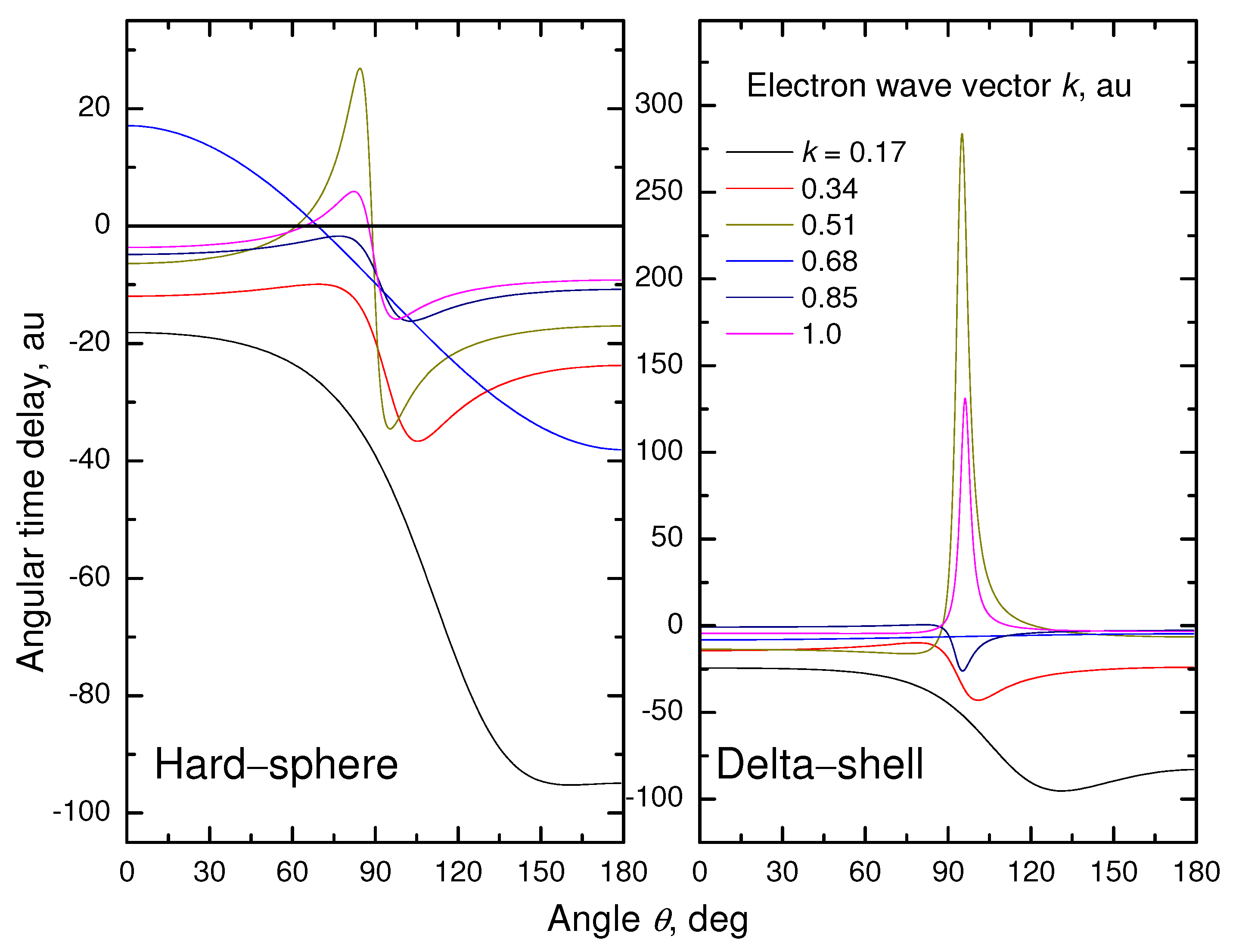
Figure 1 shows the results of the calculation by formula (9) of the angular time delay as a function of the scattering angle for some fixed electron momenta k. The left panel corresponds to the scattering on the solid sphere. The right panel corresponds to the delta-shell target. The angular time delays in these figures are given in atomic units. The atomic unit of time is equal to 24.2 attoseconds. Despite the different scales of the graphs on both panels, they show qualitatively similar behavior. The only exceptions are for the curves at . The graph of the angular dependence for the hard-sphere is almost a straight line passing from a positive to a negative half-plane at the angle of about 60, whereas on the right panel, this curve almost coincides with the x-axis. According to both panels, at low electron energies ( and 0.34), the time delay of the scattering packet is negative at all the scattering angles. The rest of the curves (except the hard-sphere target at ) are alternating for both targets. At the momenta and , the time delays on the right panel reach its maximum (∼298 atomic units (au) at in the first case and ∼140 au at the same angle in the second one). The appearance of these sharp peaks in the curves in Figure 1 is due to the almost vanishing of the denominator in the expression (9). The curves at and on the left panel cross the x-axis into the positive half-plane in the region of 90, forming a peak with a height of ~30 atomic units.
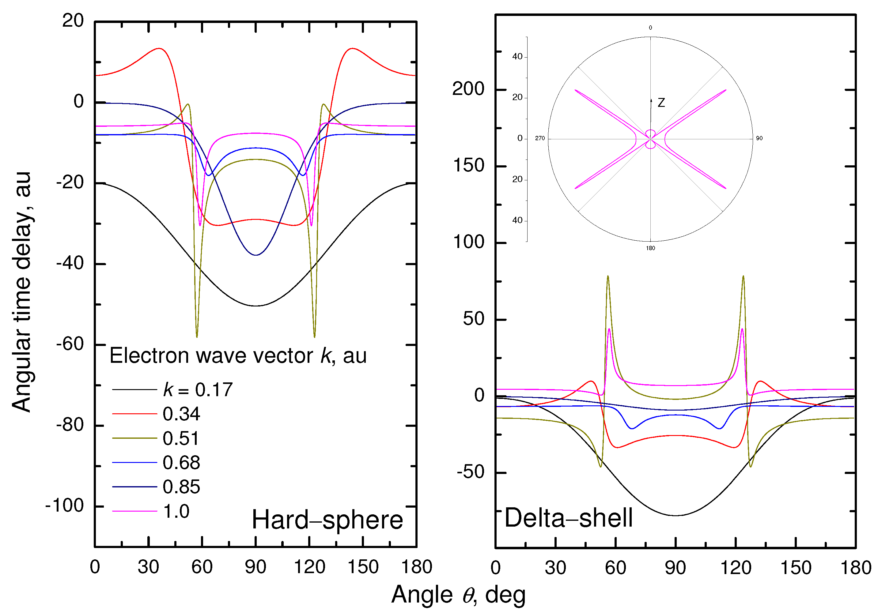
Figure 2 depicts the curves corresponding to the pair of polynomials and . We see here the results of the calculation with formula (10) of the angular time delay as a function of the scattering angle . As the sum of the orbital moments (indices of the Legendre polynomials) is an even number, the curves in Figure 2 are symmetric relative to the angle . The curves on the left panel, except for the curve at , lie entirely in the lower half-plane. The situation is quite different when the wave packet scatters by the delta-shell target. The behavior of the curve at on the right panel is particularly interesting. This curve lies entirely in the positive half-plane, which allows it to be depicted in polar coordinates (see the inset in the right panel). The 3D-picture of the function is a figure of rotation of this curve around the polar axis z, along which the incident plane wave train hits the target. The “wings of the star” shown there correspond to the polar scattering angles and 123. The qualitative similarity of the curves on both panels of Figure 2 is obvious.
Note the similarity of the curves in Figure 2 and the angular spectra in Figure 1a,b of the article in [10] (devoted to the study of angular resolved time delays in photoemission from different atomic sub-shells of noble gases). A direct comparison of the function for the processes of photoionization and elastic scattering cannot be conducted. An exclusion is the case when the dipole matrix element of photo-transitions varies slightly with the radiation frequency, and their derivatives with respect to the photon energy are negligible. Nevertheless, photoelectron spectra are similar to the scattering spectra in that they are symmetric relative to the angle . Qualitative behavior of the scattering spectrum on the delta-shell at in Figure 2 and the photoelectron spectrum in panel (a) of Figure 1 is similar. The same is to be for the curves at in Figure 1 and those in panel (b) of Figure 1 in [10].
Summarizing, we note that according to Figure 1 and Figure 2, the angular -dependencies of the function are represented by nontrivial rapidly oscillating curves lying at low electron energies mainly in the negative half-plane. The situation changes with increasing the electron energy where the dependencies become smooth.
3. -Dependence of Function
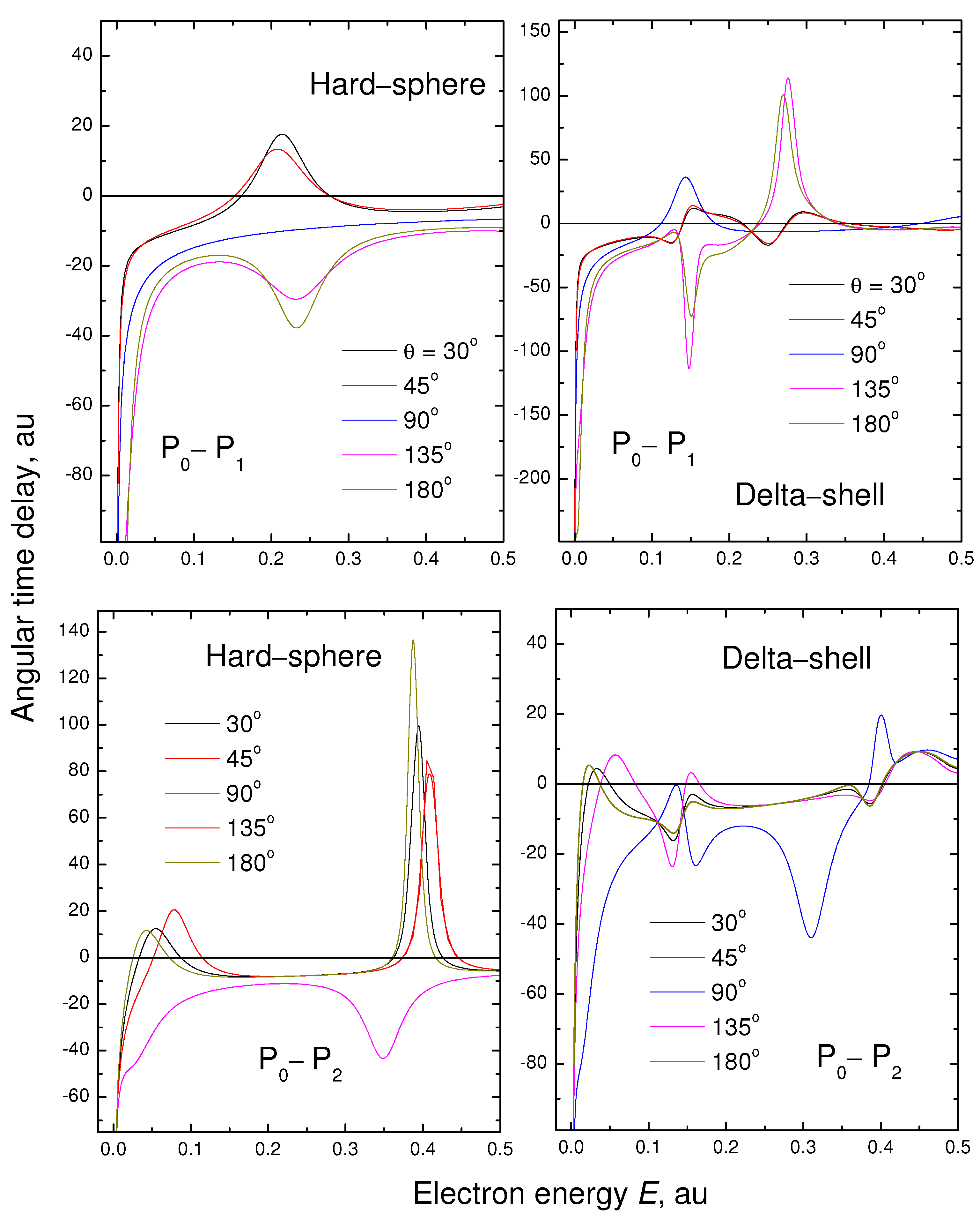
We now investigate the angular time delay as a function of the electron energy E for some fixed values of polar angles . The calculation results by formulas (9) and (10) are shown in Figure 3.
All curves in this figure tend to infinity at small electron momenta. The reason for this is that the scattering phase shift in short-range potentials must follow the Wigner threshold law [30]. In the case of s-phase shift, we have . The time delay and , that contain the derivative of the s-phase shift, for tends to infinity: . For the orbital moments the derivative of the phase shifts does vanish at the threshold as .
The left column of the figures corresponds to the electron scattering by the hard-sphere potential. The figures in the right column correspond to scattering by the delta-shell potential. In the upper right panel of Figure 3, the curves practically coincide with each other at small scattering angles , up to the angle of 45. The graphs corresponding to the angles of 135 and 180 have alternating signs, and they are characterized by the peaks in both positive and negative half-planes of the coordinate system. We see a qualitatively similar picture in the lower panel of this column where the curves for are presented. The presence of the derivative of the s-phase shift in formula (10) also leads this function to infinity at small electron energies. The curves for angles 30 and 180 almost coincide in this figure. The curve at is characterized by the maximum negative amplitude of oscillations. In the lower-left panel of Figure 3, we observe strong resonance behavior of all curves, except for the one at and energy atomic units.
In the second and third sections, we limited ourselves to the specific examples of two nonzero phases in the expansion of the wave function of a scattered electron (2) into partial waves. It is very difficult to interpret rapidly oscillating dependence of the time delays upon the energy E and scattering angle even for this simple example. An increase in the number of included essential scattering phases significantly affects the picture of the angular time delays. The increase makes the time delays rapidly oscillating when they are averaged over the energy of incident electrons. As a consequence, the scattering angle becomes inevitable to make the angular time delay observable in an experiment.
4. Average Time Delay of Scattering Process
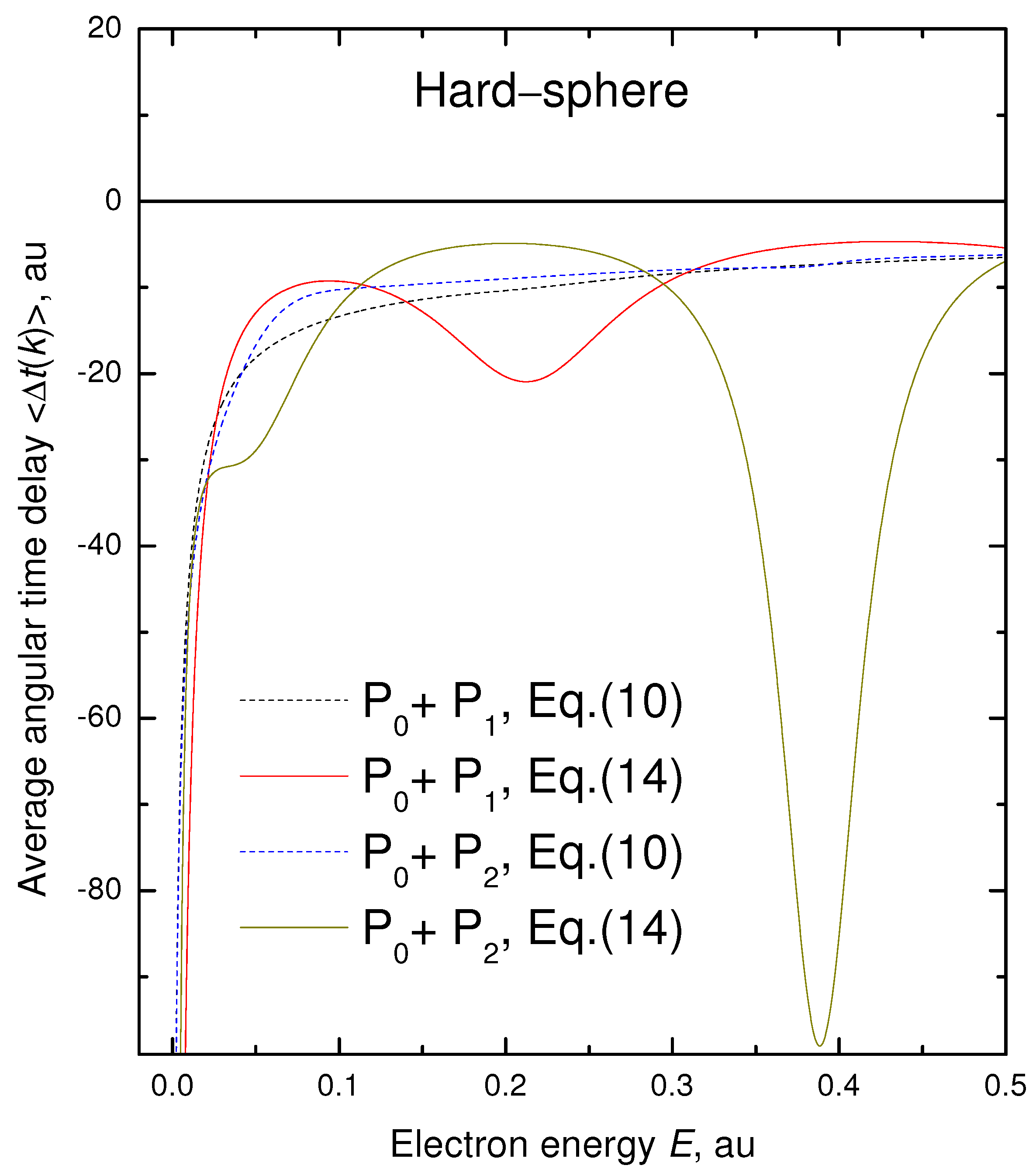
The average angular time delay is obtained from (1) by averaging over the energy spectrum of the incident wave packet, as well as over the directions weighted by the differential cross section . This averaging is reduced to the calculation of the integral of the product over all angles of electron scattering by the target and division of the obtained result by the total cross section of elastic electron scattering . The calculation of the integral is complicated by the fact that, according to (1), the function is not defined at . It was shown in [31] that the contribution to the integral from the forward scattering of an electron is determined by the real part of the scattering amplitude at zero angles. As a result of such averaging, Nussenzweig [31,32,33] obtained the expression
The second term on the left-hand side of Equation (14) eliminates the contribution of the forward scattering into the average angular time delay. Thus, the average time delay for the plane wave train is a linear combination of the EWS time delays (3). The results of the calculation of the function (14) in the case of electrons scattered by the hard-sphere target are shown in Figure 4.
Figure 4 also shows the dependencies calculated under the assumption that the statistical weight of in the sum (14) is not equal to . Instead, it is the ratio of the electron elastic scattering partial cross section to the total cross section . For more information about this assumption see, for example, Equation (10) in [10] or Equation (8) in [29]. The deep peak of the curve corresponding to the combination of the Legendre polynomials and is due to the resonant behavior of curves at au in Figure 3.
5. Concluding Remarks
Using the instructive soluble example of electron scattering by the hard-sphere potential and delta-shell potential well, we for the first time explicitly obtained the angular time-delay in terms of the scattering phase shifts and their energy derivatives . We demonstrated the complexity of as a function of the incoming electron energy E and the scattering angle . We saw that and the function , even averaged over proper intervals of E and , are more sensitive to the scattering phases than the absolute cross section and even the differential in angle scattering cross section that is proportional to . This is because the time delay functions depend not only on the cross section phases, but also upon their energy derivatives. This makes theoretical and experimental investigation of time delays a promising direction of research in the area of atomic scattering.
Author Contributions
M.Y.A., A.S.B. and I.W. contributed equally. All authors have read and agreed to the published version of the manuscript.
Funding
This research received no external funding.
Institutional Review Board Statement
Not applicable.
Informed Consent Statement
Not applicable.
Data Availability Statement
Data are available upon request.
Acknowledgments
In this section you can acknowledge any support The authors are thankful to Eric Morrow for proofreading the manuscript.
Conflicts of Interest
The authors declare no conflict of interest.
References
- Schultze, M.; Fieß, M.; Karpowicz, N.; Gagnon, J.; Korbman, M.; Hofstetter, M.; Neppl, S.; Cavalieri, A.L.; Komninos, Y.; Mercouris, T.; et al. Delay in photoemission. Science 2010, 328, 1658–1662. [Google Scholar] [CrossRef] [PubMed]
- Cavalieri, A.L.; Muller, N.; Uphues, T.; Yakovlev, V.; Baltuska, A.; Horvath, B.; Schmidt, B.; Blumel, L.; Holzwarth, R.; Hendel, S.; et al. Attosecond spectroscopy in condensed matter. Nature 2007, 449, 1029–1032. [Google Scholar] [CrossRef] [PubMed]
- Kheifets, A.S. Time delay in valence-shell photoionization of noble-gas atoms. Phys. Rev. A 2013, 87, 063404. [Google Scholar] [CrossRef] [Green Version]
- Heuser, S.; Galan, A.J.; Cirelli, C.; Marante, C.; Sabbar, M.; Boge, R.; Lucchini, M.; Gallmann, L.; Ivanov, I.; Kheifets, A.; et al. Angular dependence of photoemission time delay in helium. Phys. Rev. A 2016, 94, 063409. [Google Scholar] [CrossRef] [Green Version]
- Busto, D.; Vinbladh, J.; Zhong, S.; Isinger, M.; Nandi, S.; Maclot, S.; Johnsson, P.; Gisselbrecht, M.; L’Huillier, A.; Lindroth, E.; et al. Fano’s propensity rule in angle-resolved attosecond pump-probe photoionization. Phys. Rev. Lett. 2019, 123, 133201. [Google Scholar] [CrossRef] [PubMed] [Green Version]
- Fuchs, J.; Douguet, N.; Donsa, S.; Martin, F.; Burgdörfer, L.; Argenti, L.; Cattaneo, L.; Keller, U. Time delays from one-photon transitions in the continuum. Optica 2020, 7, 154–161. [Google Scholar] [CrossRef]
- Cirelli, C.; Marante, C.; Heuser, S.; Petersson, L.; Galan, A.J.; Argenti, L.; Zhong, S.; Busto, D.; Isinger, M.; Nandi, S.; et al. Anisotropic photoemission time delays close to a Fano resonance. Nat. Commun. 2018, 9, 955. [Google Scholar] [CrossRef]
- Ivanov, I.A. Time delay in strong-field photoionization of a hydrogen atom. Phys. Rev. A 2011, 83, 023421. [Google Scholar] [CrossRef]
- Dahlström, J.M.; Lindroth, E. Study of attosecond delays using perturbation diagrams and exterior complex scaling. J. Phys. B At. Mol. Opt. Phys. 2014, 47, 124012. [Google Scholar] [CrossRef] [Green Version]
- Wätzel, J.; Moskalenko, A.S.; Pavlyukh, Y.; Berakdar, J. Angular resolved time delay in photoemission. J. Phys. B At. Mol. Opt. Phys. 2015, 48, 025602. [Google Scholar] [CrossRef] [Green Version]
- Ivanov, I.A.; Kheifets, A.S. Angle-dependent time delay in two-color XUV+ IR photoemission of He and Ne. Phys. Rev. A 2017, 96, 013408. [Google Scholar] [CrossRef]
- Bray, A.W.; Naseem, F.; Kheifets, A.S. Simulation of angular-resolved RABBITT measurements in noble-gas atoms. Phys. Rev. A 2018, 97, 063404. [Google Scholar] [CrossRef] [Green Version]
- Hockett, P. Angle-resolved RABBITT: Theory and numerics. J. Phys. B At. Mol. Opt. Phys. 2017, 50, 154002. [Google Scholar] [CrossRef] [Green Version]
- Froissart, M.; Goldberger, M.L.; Watson, K.M. Spatial Separation of Events in S-Matrix Theory. Phys. Rev. 1963, 131, 2820–2826. [Google Scholar] [CrossRef]
- Landau, L.D.; Lifshitz, E.M. Quantum Mechanics, Non-Relativistic Theory, 3rd ed.; Pergamon Press: Oxford, UK, 1977. [Google Scholar]
- Eisenbud, L.E. The Formal Properties of Nuclear Collisions. Ph.D. Thesis, Princeton University, Princeton, NJ, USA, 1948. [Google Scholar]
- Wigner, E.P. Lower limit for the energy derivative of the scattering phase shift. Phys. Rev. 1955, 98, 145–147. [Google Scholar] [CrossRef]
- Smith, F.T. Lifetime matrix in collision theory. Phys. Rev. 1960, 118, 349–356. [Google Scholar] [CrossRef]
- Pazourek, R.; Nagele, S.; Bugdörfer, J. Time-resolved photoemission on the attosecond scale: Opportunities and challenges. Faraday Discuss. 2013, 163, 353–377. [Google Scholar] [CrossRef] [PubMed]
- Pazourek, R.; Nagele, S.; Bugdörfer, J. Attosecond chronoscopy of photoemission. Rev. Mod. Phys. 2015, 87, 765–802. [Google Scholar] [CrossRef]
- Deshmukh, P.C.; Banerjee, D. Time delay in atomic and molecular collisions and photoionisation/photodetachment. Int. Rev. Phys. Chem. 2020, 40, 127–153. [Google Scholar] [CrossRef]
- Deshmukh, P.C.; Mandal, A.; Saha, S.; Kheifets, A.S.; Dolmatov, V.K.; Manson, S.T. Attosecond time delay in the photoionization of endohedral atoms A@C60: A probe of confinement resonances. Phys. Rev. A 2014, 89, 053424. [Google Scholar] [CrossRef] [Green Version]
- Hockett, P.; Frumker, E.; Villeneuve, D.M.; Corkum, P.B. Time delay in molecular photoionization. J. Phys. B At. Mol. Opt. Phys. 2016, 49, 095602. [Google Scholar] [CrossRef]
- Baykusheva, D.; Wörner, H.J. Theory of attosecond delays in molecular photoionization. J. Chem. Phys. 2017, 146, 124306. [Google Scholar] [CrossRef] [PubMed] [Green Version]
- Amusia, M.Y.; Chernysheva, L.V. Time delay of photoionization by Endohedrals. JETP Lett. 2020, 112, 219–224. [Google Scholar] [CrossRef]
- Amusia, M.Y.; Baltenkov, A.S.; Woiciechowski, I.A. ArXive. Available online: https://arxiv.org/abs/2103.08528 (accessed on 2 March 2021).
- Schiff, L.I. Quantum Mechanics, 3rd ed.; McGraw-Hill: New York, NY, USA, 1968. [Google Scholar]
- Amusia, M.Y.; Baltenkov, A.S.; Krakov, B.G. Photodetachment of negative C60 ions. Phys. Lett. A 1998, 243, 99–105. [Google Scholar] [CrossRef]
- Amusia, M.Y.; Baltenkov, A.S. Time delay in electron-C60 elastic scattering in a Dirac bubble potential model. J. Phys. B At. Mol. Opt. Phys. 2019, 52, 015101. [Google Scholar] [CrossRef] [Green Version]
- Wigner, E.P. On the behavior of cross sections near thresholds. Phys. Rev. 1948, 73, 1002–1009. [Google Scholar] [CrossRef]
- Nussenzveig, H.M. Causality in nonrelativistic quantum scattering. Phys. Rev. 1968, 177, 1848–1856. [Google Scholar] [CrossRef]
- Nussenzveig, H.M. Time delay in quantum scattering. Phys. Rev. D 1972, 6, 1534–1542. [Google Scholar] [CrossRef]
- De Carvalho, C.A.A.; Nussenzveig, H.M. Time delay. Phys. Rep. 2002, 364, 83–174. [Google Scholar] [CrossRef]
Figure 1.
Angular time delay (9) as a function of the polar angle for fixed electron wave vectors k. The functions and used in (9) is the pair of Legendre polynomials in the amplitude of electron elastic scattering (2).

Figure 2.
Angular time delay (10) as a function of the polar angle for fixed electron wave vectors k. The functions and used in (10) is the pair of Legendre polynomials in the amplitude of electron elastic scattering (2). The inset in the right panel is the plot at in a polar coordinate system. The 3D-plot of the function is a figure of rotation of this curve around the polar axis z, along which the incident plane wave train hits the target.

Figure 3.
The angular time delay as a function of the electron energy E for some fixed values of the polar angle . - is the pair of Legendre polynomials in the upper panels. and are the polynomials used in both lower panels.
Figure 3.
The angular time delay as a function of the electron energy E for some fixed values of the polar angle . - is the pair of Legendre polynomials in the upper panels. and are the polynomials used in both lower panels.


Publisher’s Note: MDPI stays neutral with regard to jurisdictional claims in published maps and institutional affiliations. |
© 2021 by the authors. Licensee MDPI, Basel, Switzerland. This article is an open access article distributed under the terms and conditions of the Creative Commons Attribution (CC BY) license (https://creativecommons.org/licenses/by/4.0/).
Share and Cite
MDPI and ACS Style
Amusia, M.Y.; Baltenkov, A.S.; Woiciechowski, I. Time Delay in Electron Collision with a Spherical Target as a Function of the Scattering Angle. Atoms 2021, 9, 105. https://0-doi-org.brum.beds.ac.uk/10.3390/atoms9040105
AMA Style
Amusia MY, Baltenkov AS, Woiciechowski I. Time Delay in Electron Collision with a Spherical Target as a Function of the Scattering Angle. Atoms. 2021; 9(4):105. https://0-doi-org.brum.beds.ac.uk/10.3390/atoms9040105
Chicago/Turabian StyleAmusia, Miron Ya., Arkadiy S. Baltenkov, and Igor Woiciechowski. 2021. "Time Delay in Electron Collision with a Spherical Target as a Function of the Scattering Angle" Atoms 9, no. 4: 105. https://0-doi-org.brum.beds.ac.uk/10.3390/atoms9040105
Note that from the first issue of 2016, this journal uses article numbers instead of page numbers. See further details here.