
Analysis of the Transient Behaviour in the Numerical Solution of Volterra Integral Equations


1
Department of Mathematics and Applications, University of Naples “Federico II”, Via Cintia, I-80126 Napoli, Italy
2
Gruppo Nazionale per il Calcolo Scientifico, Istituto Nazionale di Alta Matematica, 00185 Roma, Italy
3
C.N.R. National Research Council of Italy, Institute for Computational Application “Mauro Picone”, Via P. Castellino, 111-80131 Napoli, Italy
*
Author to whom correspondence should be addressed.
†
These authors contributed equally to this work.
Axioms 2021, 10(1), 23; https://0-doi-org.brum.beds.ac.uk/10.3390/axioms10010023
Submission received: 20 January 2021
/
Revised: 15 February 2021
/
Accepted: 18 February 2021
/
Published: 23 February 2021
(This article belongs to the Special Issue Differential Models, Numerical Simulations and Applications)
Abstract
:In this paper, the asymptotic behaviour of the numerical solution to the Volterra integral equations is studied. In particular, a technique based on an appropriate splitting of the kernel is introduced, which allows one to obtain vanishing asymptotic (transient) behaviour in the numerical solution, consistently with the properties of the analytical solution, without having to operate restrictions on the integration steplength.
1. Introduction
Volterra integral equations (VIEs) of the type
and their discrete version,
are significative mathematical models for representing real-life problems involving feedback and control [1,2]. The analysis of their dynamics allows one to describe the phenomena they represent. In [3], the two equations were analysed in the unifying notation of time scales, and some results were obtained under linear perturbation of the kernel. Here, we revise this approach to obtain results on classes of linear discrete equations whose kernel can be split into a well-behaving part (the unperturbed kernel) plus a term that acts as a perturbation. The implications for numerical methods are, in general, not straightforward and pass through some restrictions on the step length. Nevertheless, here, we overcome this problem and obtain some results on the stability of numerical methods for VIEs.
The paper is organised as follows. In Section 2, we introduce the split kernel for Equation (2) and, using a new formulation of Theorem 2 in [3], we provide sufficient conditions for the above-mentioned splitting that imply that the solution vanishes. In Section 3, we propose a reformulation of the methods for (1) as discrete Volterra equations and exploit the theory developed in the previous section in order to investigate its numerical stability properties. In Section 4, some applications are described and analysed through the tools developed in Section 2 and Section 3, for which we obtain new and more general results on the asymptotic behaviour for the numerical solutions of both linear and nonlinear equations. In Section 5, some numerical examples are reported.
2. Asymptotics for Discrete Equations
Consider the discrete Volterra Equation (2) with where P and Q are matrices. Let be the resolvent kernel associated with which is defined as the solution of the equation:
The following theorem, which we proved in [3], represents the starting point of our investigation.
This theorem is particularly interesting when the matrix P in the splitting of kernel K is such that for with M and N positive constants and Then, Equation (2) can be rewritten as
and the following result holds. Here and in the following, the limit of matrices is intended element-wise.
Theorem 2.
Consider Equation (4), and assume that:
- (1)
- for and
- (2)
- for any fixed
If there exists a constant such that then
and if then
Proof.
The case and can be treated by the same technique if it is known that for (I is the identity matrix). In this case, we have the following corollary.
3. Background Material on Methods
The analysis carried out in the previous section can be effectively applied to methods for the systems of VIEs:
Here, we consider the numerical solution to (5) obtained by the methods with Gregory convolution weights (see, for example, [5,6,7]):
where with for is the step size and are the weights. We assume that the weights are non-negative and that are given starting values.
The weights are called the starting weights and satisfy (see [5]):
Moreover, we want to underline some properties of the Gregory convolution weights, (see, for example [5,7]), which will be useful in the subsequent sections:
From now on, we assume that h satisfies
where I is the identity matrix of size d.
Choose and let
and
The method (6) can be written, for as follows:
with This alternative formulation of the method in terms of matrices P and Q allows us to analyse its asymptotic properties using the theory developed in the previous paragraph for Equation (4). So, (11) corresponds to the discrete Equation (4) with M and N equal to and , respectively, and for
4. Dynamic Behaviour of Numerical Approximations and Applications
In [8], we carried out an analysis of Volterra equations on time scales that allowed us to obtain results on the asymptotic behaviour of the analytical solution of (5) and on its discrete counterpart in under the assumptions:
and
respectively, where and If is non-increasing with respect to the bound (13) is certainly implied by (12) for those values of the parameter h such that
This relation, which allows one to establish a connection between the behaviour of the analytical solution of (5) and of its discrete counterpart in does not straightforwardly apply to numerical methods due to the presence of the weights and of the methods. This is because the weights can cause the loss of monotonicity, and they may also be greater than 1; then, (13) is not satisfied. In [8], it was proved that if (12), and are satisfied, the analytical solution of Equation (5) vanishes at infinity as Moreover, in [9], it was shown that, if then there exists a positive constant A such that
The bound (14) assures that, when (12) is satisfied, the numerical solution tends to zero for if the step size h is small enough, consistently with the behaviour of .
Theorem 2 in Section 2 allows us to remove the restriction on h given by (14). In order to show this result, which states, in fact, the unconditional stability of the methods, we need the following preparatory lemma.
Lemma 1.
Assume that:
- (i)
- for any fixed ,
- (ii)
- there exists such that for
- (iii)
- there exists such that
Then, for any such that where is such that
Proof.
Let be a fixed value of the step size. Assumption (ii) implies that for any Moreover, because of (i); thus, for any we choose such that
Now, we choose such that and such that Since, for is a non-increasing function in s for each we have □
Theorem 3.
Proof.
For a fixed Lemma 1 provides a value for which with positive constant. Referring to the reformulation (11) of the method, all the assumptions of Theorem 2 are satisfied. Thus, because of property (7) on the asymptotic behaviour of starting weights and of assumption of Lemma 1, tends to zero for So, in view of Theorem 2, also vanishes. □
Other applications of Theorem 2 are concerned with the equation
which has been the subject of great attention in the literature (see, for example, [10,11,12]). Here and in the following, we assume that Equation (16) is scalar (), the kernel is of convolution type, is a continuous function for and A main assumption (see, for example, [13]) that is generally made on the nonlinear term G is that it represents a small perturbation, that is, there exists a function such that
For Equation (16), the methods with Gregory convolution weights read, for
In order to describe the asymptotic behaviour of , we prove the following theorem.
Theorem 4.
Assume that, for Equation (16), the following assumptions hold:
Hypothesis 1.
Hypothesis 2.
such that ,
Hypothesis 3.
,
Hypothesis 4.
.
Proof.
Now, consider the equation
Since, from (8), are bounded, we have that which is the convolution product of an () and a vanishing () sequence and, therefore, tends to zero as Therefore, We choose such that and such that in assumption With the equation for can be written in the more convenient form, (11), for which all the assumptions of Theorem 2 hold. Thus, because of property (7) on the asymptotic behaviour of starting weights and because of the vanishing behaviour of the kernel tends to zero for Therefore, This ends the proof because, using the comparison theorem in [14], □
This theorem states that the numerical solution of (16) vanishes when the forcing term f tends to zero for any step size . The result is, of course, more interesting if we know that the analytical solution to (16) tends to zero. This can be proved by means of a result that the authors proved in [8]. To be more specific, the assumptions of Theorem 4 here assure that all the hypotheses of Theorem 9 in [8] are satisfied, thus implying that
The following result, which we prove in the case of scalar equations, represents a generalisation of Theorem in [15], where the numerical stability of the methods up to order 3 was proved under some restriction on the step length In this paper, by applying Theorem 2 to the (6), we remove the constraint on the step size, and extend the investigation to any method in the class of
Theorem 5.
Assume that, for Equation (5), with it holds that:
- (i)
- such that
- (ii)
- ,
- (iii)
- ,
- (iv)
Then. for the numerical solution obtained with the (6), it holds that
Proof.
Due to hypotheses (i) and (ii), there exists such that
Let us fix From the assumptions, it is clear that with So, (ii) implies that for some which we choose such that Since, for (iii), is a non-increasing function, we have
Then, referring to formulation (11) of the numerical method with we want to prove that
Here, ; thus, So, (21) is guaranteed by (20). Furthermore, in view of (19), it is for any fixed and, because of (ii) and (iii), also Hence, as all the assumptions of Theorem 2 are accomplished, without imposing any restriction on the step size
If, however, assumption (iii) holds instead of (iii) the step size h has to be chosen such that and with So, by Lemma 1 in [9],
□
Consider now the following convolution equation:
Its solution has the form
where the resolvent kernel R is the solution of the equation:
If the kernel of Equation (22) is completely monotone, that is, then (see, e.g., [16]) the resolvent is also completely monotone. Furthermore, the analytical solution and its numerical approximation obtained by a method both tend to zero as and respectively, when the forcing term tends to zero (see [6]). We point out that if then as well, as is the solution of a Volterra Equation (23) where the kernel is completely monotone and the forcing tends to zero. The significance of completely monotone kernels in Volterra equations is underlined in [13] (p. 27).
A nonlinear perturbation to (22) yields
This equation can be written in terms of the unperturbed solution as (see [13]):
Starting from assumption (17) on the nonlinear term and from the relation (25), we want to investigate the asymptotic behaviour of the numerical solution to (24) when it is known that
Theorem 6.
- 1.
- is completely monotone and ,
- 2.
- .
If then the solution and the numerical solution obtained by the method (6) satisfy
Proof.
For assumption the solution of Equation (22) with a completely monotone kernel satisfies This also holds true for its numerical approximation (see, for example, [6]).
Considering Equation (25), it is
Since is completely monotone and is bounded, the solution of the equation
satisfies By using the comparison theorem (see, for example, [17]), also tends to zero. Considering the numerical solution of (26), we want to show, by means of Theorem 5, that Then, will also vanish.
This is true because all the assumptions of Theorem 5 are satisfied. Indeed:
- (i)
- thus, and ; as a matter of fact, as R is the resolvent of a completely monotone vanishing kernel, it is, in turn, a completely monotone vanishing kernel.
- (ii)
- since assumption holds,
- (iii)
- since assumption holds,
- (iv)
- as pointed out before, as it is the solution of the linear VIE (22), with a completely monotone kernel and vanishing forcing term.
□
5. Numerical Examples
In this section, we report some numerical experiments in order to experimentally prove the theoretical results illustrated in Section 4. For our experiments, we choose illustrative test equations and we use the method (6) with trapezoidal weights.
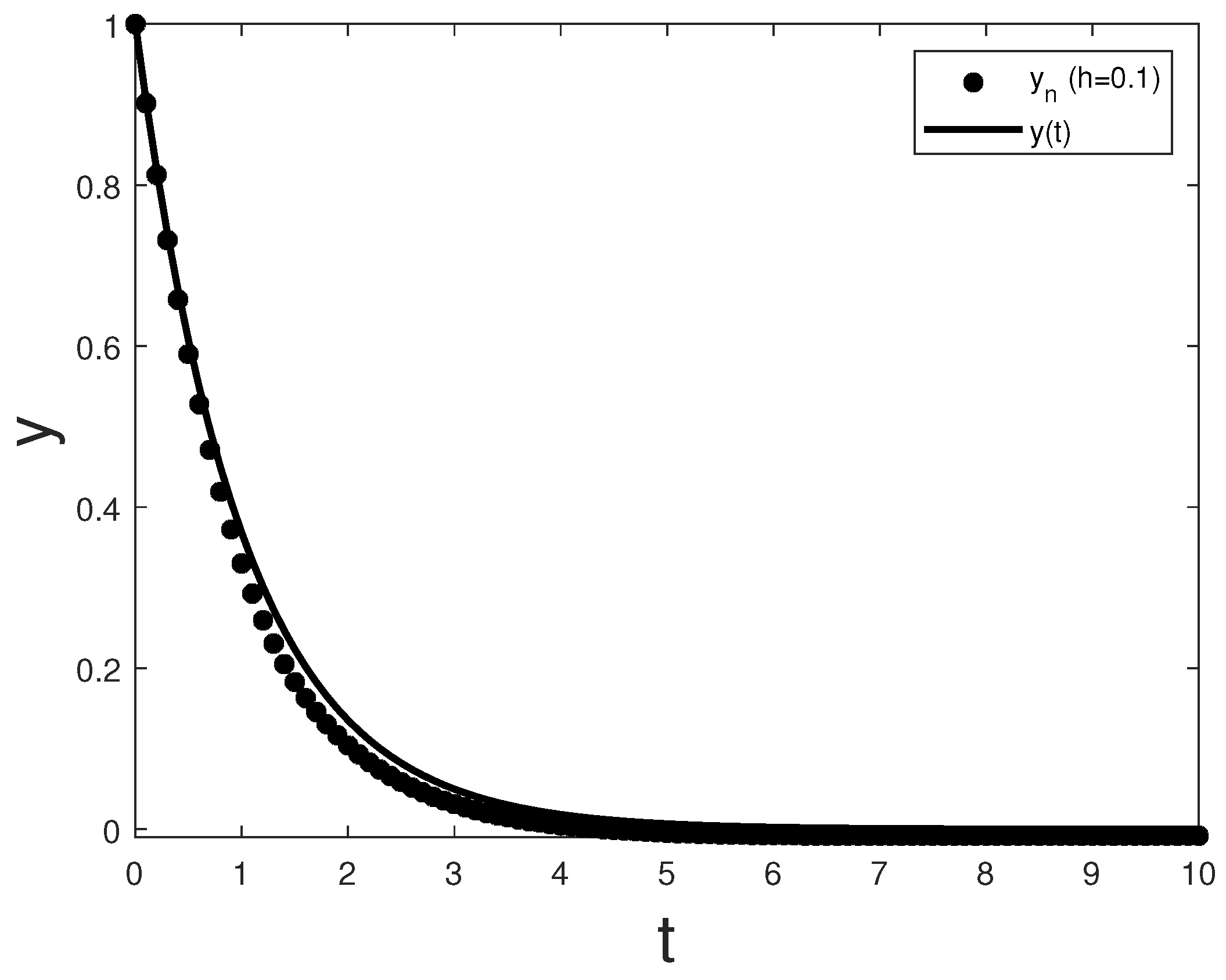
In our first example, we refer to Equation (5) with the kernel k given by
and the forcing term such that the solution Since tends to zero as t goes to infinity, all the assumptions of Theorem 3 are satisfied (for example, with ), and thus, both the numerical solution and the continuous one vanish. This is also clear in Figure 1.
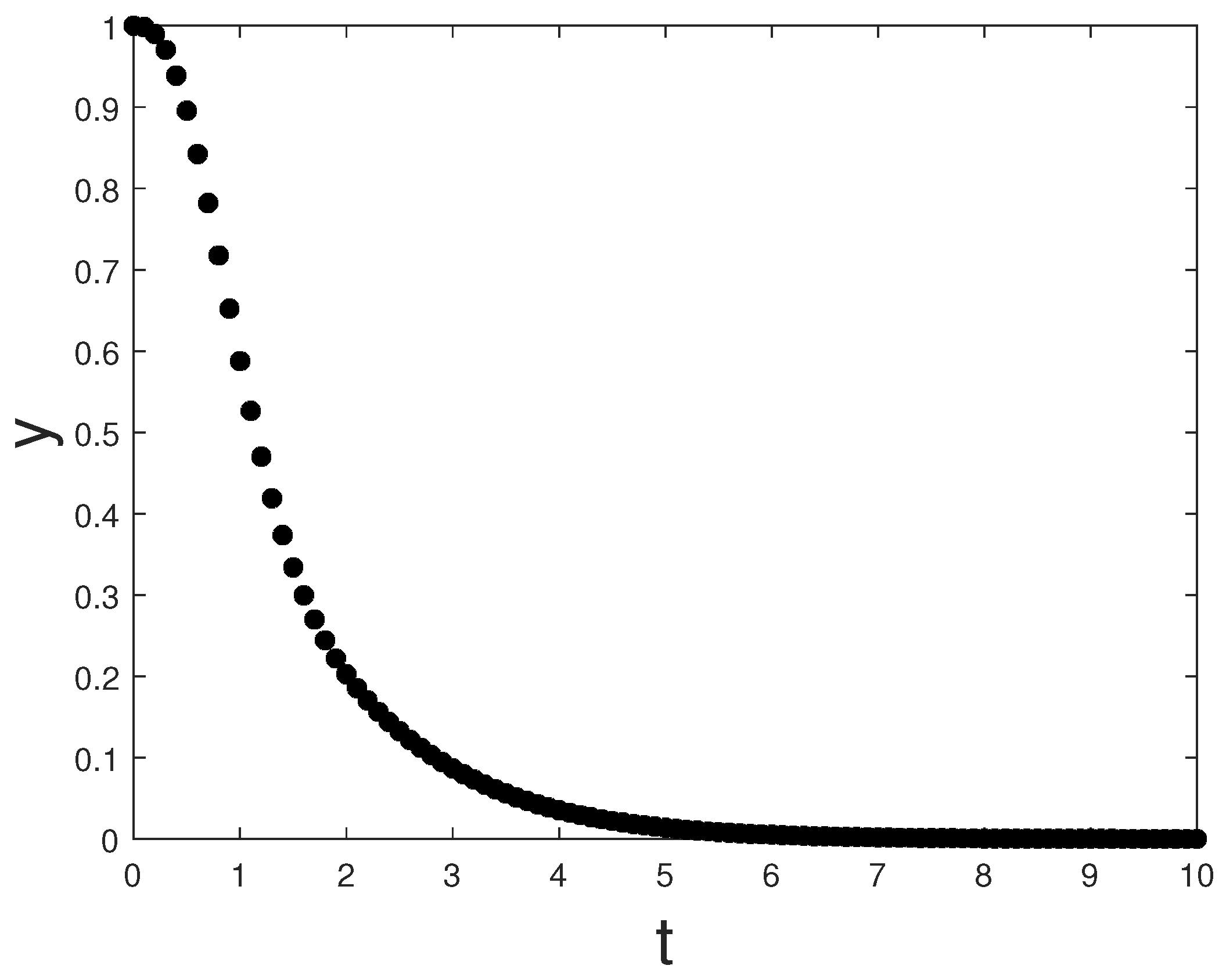
Now, consider Equation (16) with
In Figure 2, we draw the numerical solution obtained with step size which clearly vanishes at infinity, according to Theorem 4, since all assumptions are accomplished with and
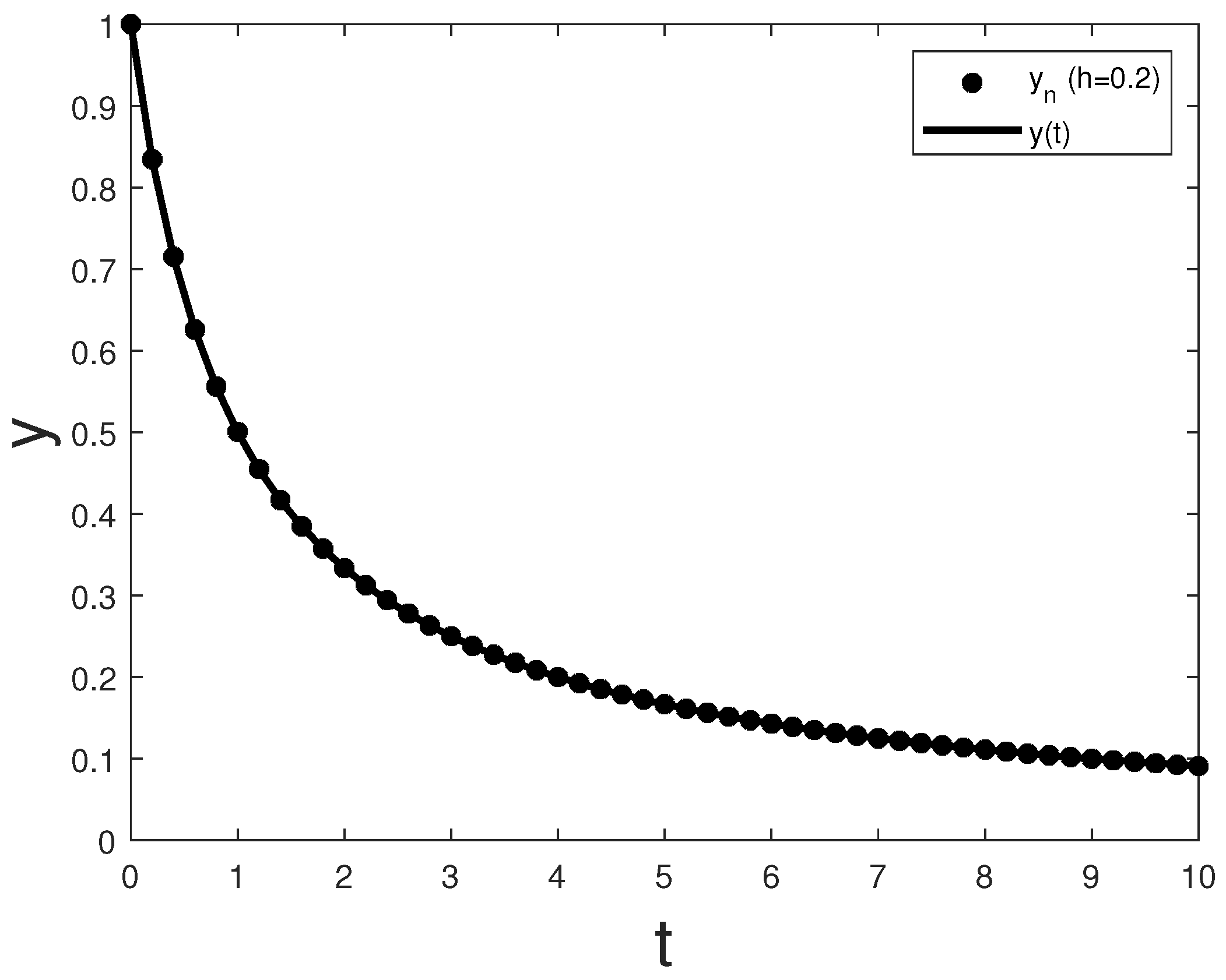
Our third example consists in Equation (5) with
and such that the solution According to Theorem 5, with since tends to zero, the numerical solution vanishes regardless of the step size thus replicating the asymptotic behaviour of the continuous one. This behaviour is shown in Figure 3.
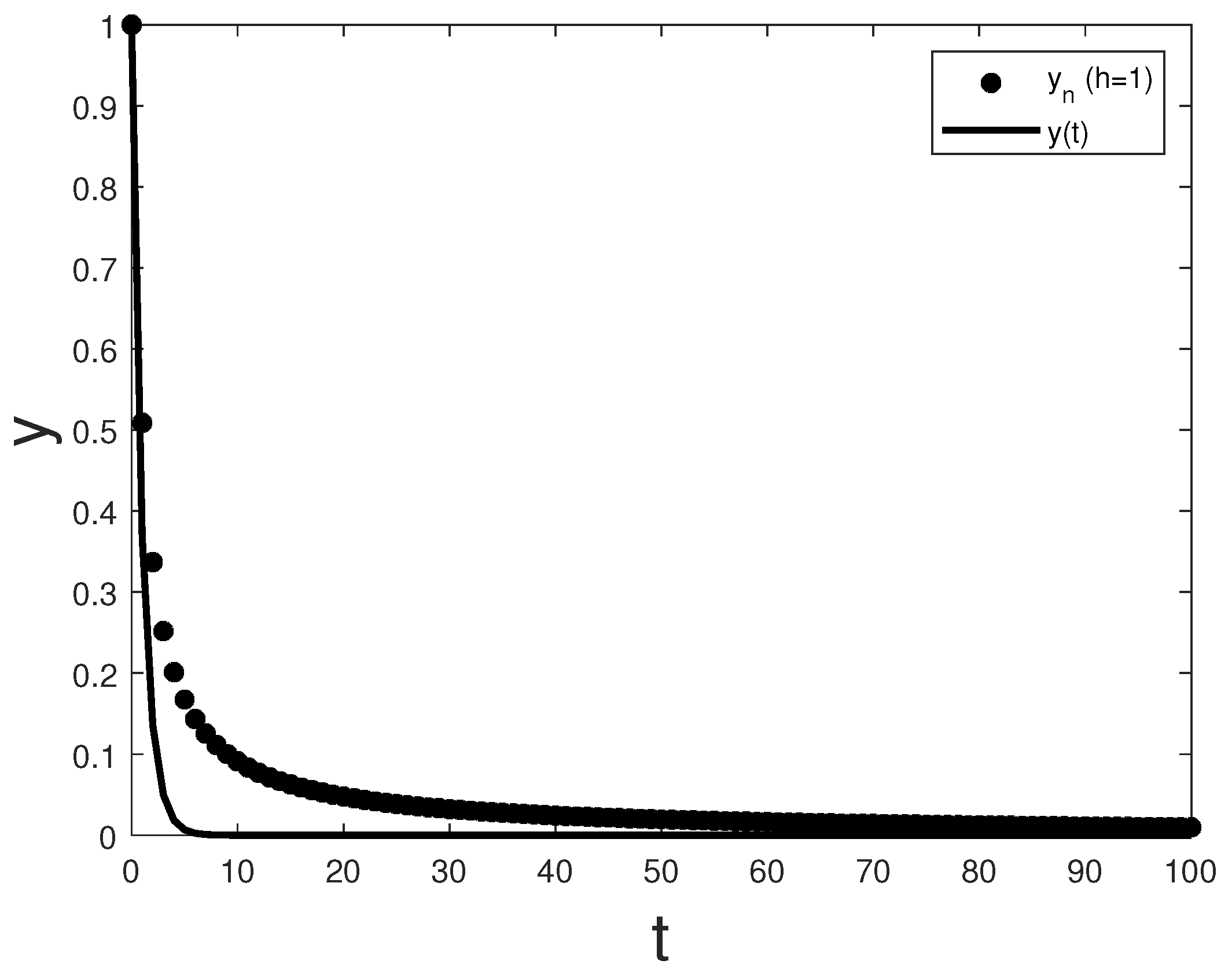
In all our experiments, we used sizes for the meshes that ensure reasonable accuracy in the numerical solution at finite times. Integration with larger discretisation steps naturally introduces greater errors on finite time intervals, but the numerical solution maintains the expected behaviour at infinity. Thus, this confirms the asymptotic-preserving characteristics of the numerical schemes without restrictions on This can be observed, for example, in Figure 4, again referring to example (29) with
6. Conclusions
Starting from an idea developed in [3], here, we have introduced a technique for the analysis of the vanishing behaviour of the numerical solution to VIEs. This new approach, which is based on suitable splittings of the kernel function, allows one to preserve the character of the analytical solution even in the weighted sums that appear in the method, thus leading to unconditional stability results in many applications of interest.
Author Contributions
Both authors contributed equally to this work. Both authors have read and agreed to the published version of the manuscript.
Funding
This research was funded by the INdAM-GNCS 2020 project “Metodi numerici per problemi con operatori non locali”.
Acknowledgments
The authors are grateful to the anonymous reviewers for their constructive comments, which helped to improve the manuscript.
Conflicts of Interest
The authors declare no conflict of interest.
References
- Gripenberg, G.; Londen, S.O.; Staffans, O. Volterra Integral and Functional Equations; Cambridge University Press: Cambridge, UK, 1990. [Google Scholar]
- Elaydi, S. An Introduction to Difference Equations; Springer: New York, NY, USA, 2005. [Google Scholar]
- Messina, E.; Raffoul, Y.; Vecchio, A. Analysis of Perturbed Volterra Integral Equations on Time Scales. Mathematics 2020, 8, 1133. [Google Scholar] [CrossRef]
- Gyori, I.; Reynolds, D. On admissibility of the resolvent of discrete Volterra equations. J. Differ. Equ. Appl. 2010, 16, 1393–1412. [Google Scholar] [CrossRef]
- Brunner, H.; van der Houwen, P. The Numerical Solution of Volterra Equations; North-Holland: Amsterdam, The Netherlands, 1986. [Google Scholar]
- Lubich, C. On the stability of linear multistep methods for Volterra convolution equations. IMA J. Numer. Anal. 1983, 3, 439–465. [Google Scholar] [CrossRef]
- Wolkenfelt, P.H.M. Linear Multistep Methods and the Construction of Quadrature Formulae for Volterra Integral and Integro-Differential Equations; Report NW 76/79; Mathematisch Centrum: Amsterdam, The Netherlands, 1979. [Google Scholar]
- Messina, E.; Vecchio, A. Stability and Convergence of Solutions to Volterra Integral Equations on Time Scales. Discret. Dyn. Nat. Soc. 2015, 2015, 6. [Google Scholar] [CrossRef] [Green Version]
- Messina, E.; Vecchio, A. A sufficient condition for the stability of direct quadrature methods for Volterra integral equations. Numer. Algorithms 2017, 74, 1223–1236. [Google Scholar] [CrossRef] [Green Version]
- Agyingi, E.; Baker, C. Derivation of variation of parameters formulas for non-linear Volterra equations, using a method of embedding. J. Integral Equ. Appl. 2013, 25, 159–191. [Google Scholar] [CrossRef]
- Miller, R. A nonlinear variation of constants formula for Volterra equations. Math. Syst. Theory 1972, 6, 226–234. [Google Scholar]
- Miller, R. On the linearization of Volterra integral equations. J. Math. Anal. Appl. 1968, 23, 198–208. [Google Scholar] [CrossRef] [Green Version]
- Burton, T. Kernel-Resolvents relations for an integral equation. Tatra Mt. Math. Publ. 2011, 48, 25–40. [Google Scholar] [CrossRef] [Green Version]
- Brunner, H. Collocation Methods for Volterra Integral and Related Functional Differential Equations; Cambridge University Press: Cambridge, UK, 2004. [Google Scholar]
- Vecchio, A. Volterra discrete equations: Summability of the fundamental matrix. Numer. Math. 2001, 89, 783–794. [Google Scholar] [CrossRef]
- Gripenberg, G. On Positive, Nonincreasing Resolvents of Volterra Equations. J. Differ. Equ. 1978, 30, 380–390. [Google Scholar] [CrossRef] [Green Version]
- Brunner, H. Volterra Integral Equations: An Introduction to Theory and Applications; Cambridge Monographs on Applied and Computational Mathematics; Cambridge University Press: Cambridge, UK, 2017. [Google Scholar] [CrossRef]
Figure 1.
Numerical solution to problem (27) compared to the analytical one.
Figure 1.
Numerical solution to problem (27) compared to the analytical one.

Figure 2.
Numerical solution to problem (28) with
Figure 2.
Numerical solution to problem (28) with

Figure 3.
Numerical solution to problem (29) with h = 0.2, compared to the analytical one.
Figure 3.
Numerical solution to problem (29) with h = 0.2, compared to the analytical one.

Figure 4.
Numerical solution to problem (29) with h = 1, compared to the analytical one.
Figure 4.
Numerical solution to problem (29) with h = 1, compared to the analytical one.

Publisher’s Note: MDPI stays neutral with regard to jurisdictional claims in published maps and institutional affiliations. |
© 2021 by the authors. Licensee MDPI, Basel, Switzerland. This article is an open access article distributed under the terms and conditions of the Creative Commons Attribution (CC BY) license (http://creativecommons.org/licenses/by/4.0/).
Share and Cite
MDPI and ACS Style
Messina, E.; Vecchio, A. Analysis of the Transient Behaviour in the Numerical Solution of Volterra Integral Equations. Axioms 2021, 10, 23. https://0-doi-org.brum.beds.ac.uk/10.3390/axioms10010023
AMA Style
Messina E, Vecchio A. Analysis of the Transient Behaviour in the Numerical Solution of Volterra Integral Equations. Axioms. 2021; 10(1):23. https://0-doi-org.brum.beds.ac.uk/10.3390/axioms10010023
Chicago/Turabian StyleMessina, Eleonora, and Antonia Vecchio. 2021. "Analysis of the Transient Behaviour in the Numerical Solution of Volterra Integral Equations" Axioms 10, no. 1: 23. https://0-doi-org.brum.beds.ac.uk/10.3390/axioms10010023
Note that from the first issue of 2016, this journal uses article numbers instead of page numbers. See further details here.