
Enumeration of the Additive Degree–Kirchhoff Index in the Random Polygonal Chains


School of Mathematics and Big Data, Anhui University of Science & Technology, Huainan 232002, China
*
Author to whom correspondence should be addressed.
Axioms 2022, 11(8), 373; https://0-doi-org.brum.beds.ac.uk/10.3390/axioms11080373
Submission received: 23 June 2022
/
Revised: 23 July 2022
/
Accepted: 26 July 2022
/
Published: 28 July 2022
(This article belongs to the Special Issue Graph Theory with Applications)
Abstract
:The additive degree–Kirchhoff index is an important topological index. This paper we devote to establishing the explicit analytical expression for the simple formulae of the expected value of the additive degree–Kirchhoff index in a random polygon. Based on the result above, the additive degree–Kirchhoff indexes of all polygonal chains with extremal values and average values are obtained.
Keywords:
additive degree–Kirchhoff index; random polygonal chains; expected value; extremal value; average valueMSC:
05C501. Introduction
In this paper, we only consider simple and finite connected graphs. The topology and chemical index of the graph play important roles in describing the chemical molecular diagram and establishing the relationships between molecular structure and characteristics. It is a topological index closely related to the physical and chemical properties of compounds, so it is widely used to predict the physical and chemical properties and biological activity of compounds.
The molecular diagram in a chemical diagram is the structural diagram of a compound molecule. We let the vertices represent the atoms, and edges stand for the covalent bonds between atoms. Then, the molecular structure can be represented by this diagram, which is called the molecular diagram. For more detailed information, we can refer to [1,2,3,4,5,6,7,8,9,10,11,12,13] and the references cited therein.
The molecular topological index is a kind of topological invariant, which is a numerical parameter generated from a molecular structure, and the properties of molecules are indirectly expressed by molecular structure—that is, the relationship between molecular structure and performance can be established. The physical and chemical properties of molecules can be reflected by some topological indexes, which can be divided into many categories according to different parameters, such as point degree, adjacent point degree and the distance between two points. Let be a graph with the vertex set and the edge set . The degree (or for short) of a vertex v in G is the number of edges of G incident with v.
In 1993, the resistance distance was found to be a novel distance function on the graph proposed by Klein and Randić [14]. denotes the resistance distance between vertices x and y in G. For , the resistance distance between x and y in G, denoted by , is defined as the effective resistance between nodes x and y of the electrical network, for which nodes corresponding to vertices of G and each edge of G are replaced by resistors of unit resistance. The Kirchhoff index of G is defined in analogy to the Wiener index as [15,16,17,18,19,20,21]
In 2012, the additive degree–Kirchhoff index was introduced by Gutman, Feng and Yu. We refer the papers [22,23], in which it was defined as
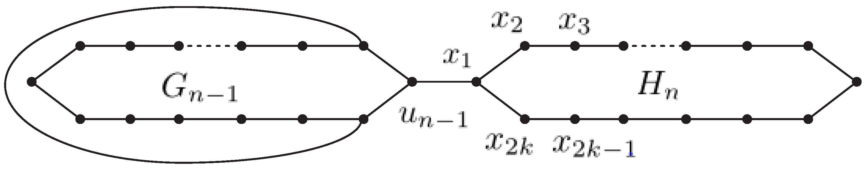
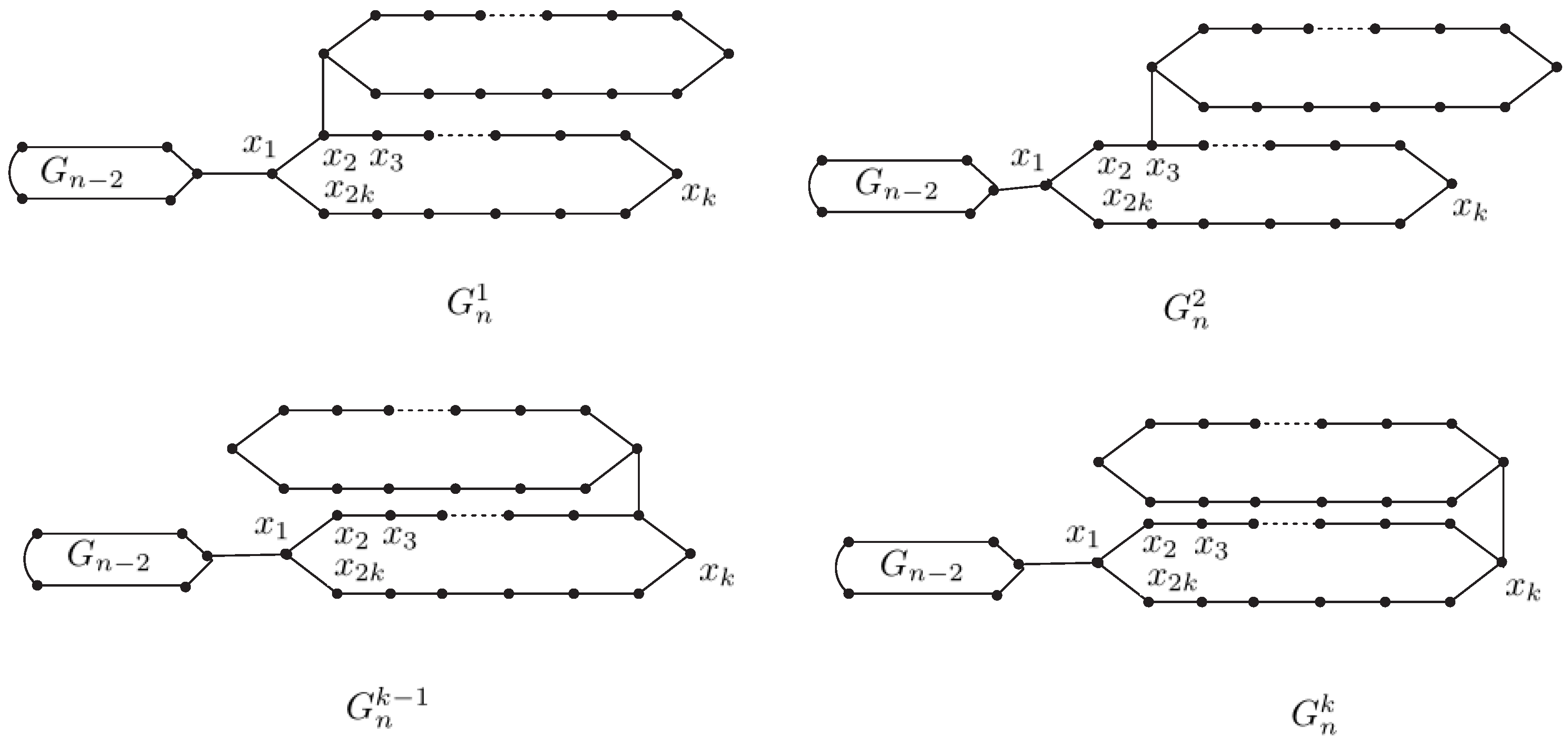
A random polygonal chain with n polygons can be regarded as a polygonal chain with polygons to which a new terminal polygon has been adjoined by a cut edge; see Figure 1. For , the terminal polygon can be attached in k ways, which results in the local arrangements we describe as , , , …, See Figure 2. A random polygonal chain with n polygons is a polygonal chain obtained by stepwise addition of terminal polygons. At each step , a random selection is made from one of the k possible constructions:
- with probability ,
- with probability ,
- with probability ,
- ⋮ ⋮ ⋮
- with probability ,
- with probability ,
where the probabilities , , , …, are constants, unrelated to the step parameter k.
Let be a polygonal chain with n polygons , , …, . Set as the cut edge of connecting and with , for . Clearly, both and are the vertices in and . In particular, is the meta-chain ; the ortho-chains are , , …; and the para-chain is if (i.e., ), = 2 (i.e., ), = 3 (i.e., ), …, = k (i.e., ) for all , respectively. For convenience, let be the set of all polygonal chains with n polygons.
Huang, Kuang and Deng [24,25] obtained the expected values of the Kirchhoff index of random polyphenyl and spiro chains. Zhang and Li et al. [26], obtained the expected values of the expected values for the Schultz index, Gutman index, multiplicative degree–Kirchhoff index and additive degree–Kirchhoff index of a random polyphenylene chain. For more information, we can refer to [27,28,29,30,31,32,33,34]. The molecular diagram in this paper contains all the molecular diagrams of the previous study and is a general result. We calculate the explicit analytical expressions for the expected values of the additive degree–Kirchhoff index of a random polygonal chain. We also obtained the extremal values and average values of the additive degree–Kirchhoff index with respect to the set of all polygonal chains with n polygons. It can be applied in practice more conveniently. These results can help biochemists with predicting and synthesizing new compounds and drugs.
2. The Additive Degree–Kirchhoff Index in a Random Polygonal Chain
In this section, we consider the expected value of additive degree–Kirchhoff index of the random polygonal chain. For a random polygonal chain , the additive degree–Kirchhoff index is a random variable. In fact, is linked to a new terminal polygonal by an edge, where is spanned by vertices , , , …, , and the new edge is ; see Figure 1. On the one hand, for all , one has
On the other hand,
Theorem 1.
For , the expected value for the additive degree–Kirchhoff index of the random polygonal chain is
Proof.
Recall that the random polygonal chain is obtained by attaching to a new terminal polygonal by an edge, where is spanned by vertices , , , …, , and the new edge is ; we may use the same notation as that used at the beginning of last section. By (2), one has
Note that
Recall that and for . From (3) and (4), we have
Note that for . From (5), one has
Then,
For a random polygonal chain , the number is a random variable. We may denote its expected value by
For a random polygonal chain , the number is a random variable. We may denote its expected value by
By a expectation operator and by substituting and into (6), we can obtain a recurrence relation for the expected value for the additive degree–Kirchhoff index of a random polygonal chain as follows:
Consider the following k possible cases.
- Case 1.
- . In this case, coincides with the vertex or . Consequently, is given by or with probability .
- Case 2.
- . In this case, coincides with the vertex or . Consequently, is given by or with probability .
- Case 3.
- . In this case, coincides with the vertex or . Consequently, is given by or with probability .
- ⋮ ⋮ ⋮
- Case k − 3.
- . In this case, coincides with the vertex or . Consequently, is given by or with probability .
- Case k − 2.
- . In this case, coincides with the vertex or . Consequently, is given by or with probability .
- Case k − 1.
- . In this case, coincides with the vertex or . Consequently, is given by or with probability .
- Case k.
- , then is the vertex . Consequently, is given by with probability .
According to the above k cases, we may obtain the expected value as
By applying the expectation operator to the above equation, and noting that , we obtain
Let
Hence,
The boundary condition is
According to the above recurrence relation and the boundary condition, we have
Thus,
According to the above and the above k cases, we may obtain the expected value as
By applying the expected operator to the above equation, and noting that , we obtain
Let
Hence,
The boundary condition is
According to the above recurrence relation and the boundary condition, we have
Thus,
Therefore,
and the boundary condition is .
According to the above recurrence relation and the boundary condition, we have
Let
Hence,
as desired. □
If we set = , , , , respectively, and by Theorem 1, we can receive the additive degree–Kirchhoff indexes of the meta-chain ; the ortho-chain , , …, ; and the para-chain , as
Through observation and direct calculation, we have
Corollary 1.
For a random polygonal chain , the para-chain realizes the maximum of , and the meta-chain realizes that of the minimum.
Proof.
By Theorem 1, we have
Note that , so by taking the partial derivative, one has
When (i.e., ), the para-chain realizes the maximum of ; that is, . If , let . Then, we have
Therefore,
Thus, (i.e., ), and cannot attain the minimum value. With the same calculations as the same above, if , let , . Then, we have
Therefore,
Only when , may we get to the minimum value. Then, let
Thus,
Thus, achieves the minimum value when (i.e., = 1); that is, . □
3. The Average Value for the Additive Degree–Kirchhoff Index
Recall that is the set of all polygonal chains with n polygons. In this section, we give the average value for the additive degree–Kirchhoff index with respect to .
In order to achieve the average value , it takes in the expected value for the additive degree–Kirchhoff index of the random polygonal chain . According to Theorem 1, we have:
Theorem 2.
For , the average value for the the additive degree–Kirchhoff indexes with respect to are
After verification, the equations are established:
4. Concluding Remarks
Most of the published papers are about the study of polyphenylene and cyclooctatetraene chains; the results are not generic. In this paper, we obtained the explicit analytical expression for the expected values of the additive degree–Kirchhoff index as a random polygonal chain. We also obtained the extremal values and average values of the index. All the research can better predict the physicochemical properties of more novel compounds, which can be applied to the research of drugs, macromolecular polymers and new materials.
In chemical graph theory, the matter of a polygonal chain is being widely studied by researchers. The molecular structures of polygonal chemicals are various, and its physicochemical properties also become more and more important, and refer to [35,36,37]. The graph invariant not only presents vast potential for structure–activity and structure–property relationships, but also offers precious leads for the advancement of safe and potent curative of multiple nature as well. By this paper is possible to establish exact formulas for the expected values of some indices of a random polygon chain with n regular polygons.
In reverse engineering of pharmaceuticals and nanomaterials—refer to [38,39,40,41]—scientists hope to create certain drugs or test the performance of a nanometer material. They can use the method of this study by extending it to a certain topological index (corresponding to certain features of drugs or material) with expected values, extremal values and average values, getting the structures of the target compounds from the point of view of mathematics and then synthesizing the targeted chemicals.
Author Contributions
The authors contributed equally to this article. All authors have read and agreed to the published version of the manuscript.
Funding
The research is partially supported by National Science Foundation of China (grant number 12171190), the Graduate innovation fund project of Anhui University of Science and Technology (grant number 149), the Natural Science Foundation of Anhui Province (grant number 2008085MA01) and funded by Research Foundation of the Institute of Environment-friendly Materials and Occupational Health (Wuhu), Anhui University of Science and Technology (Grant No. ALW2021YF09).
Conflicts of Interest
The authors declare that they have no competing interest.
References
- Bai, Y.; Zhao, B.; Zhao, P. Extremal Merrifield-Simmons index and Hosoya index of polyphenyl chains. Match Commun. Math. Comput. Chem. 2009, 62, 649–656. [Google Scholar]
- Bondy, J.; Murty, U. Graph Theory (Graduate Texts in Mathematics); Springer: New York, NY, USA, 2008; Volume 244. [Google Scholar]
- Chen, A.; Zhang, F. Wiener index and perfect matchings in random phenylene chains. Match Commun. Math. Comput. Chem. 2009, 61, 623–630. [Google Scholar]
- Chung, F.R.K. Spectral Graph Theory CBMS Series; American Mathematical Society: Philadelphia, PA, USA, 1997; Volume 92. [Google Scholar]
- Entringer, R.C.; Jackson, D.E.; Snyder, D. Distance in graphs. Czechoslov. Math. J. 1976, 26, 283–296. [Google Scholar] [CrossRef]
- Buckley, F.; Harary, F. Distance in Graphs. In Structural Analysis of Complex Networks; Addison-Wesley: Redwood City, CA, USA, 1990. [Google Scholar]
- Wei, S.; Shiu, W.C. Enumeration of Wiener indices in random polygonal chains. J. Math. Anal. Appl. 2019, 469, 537–548. [Google Scholar] [CrossRef]
- Estrada, E.; Bonchev, D. Chemical Graph Theory. In Discrete Mathematics and Its Applications Series; Taylor & Francis: London, UK, 2013; No. 83. [Google Scholar]
- Evans, W.C.; Evans, D. Hydrocarbons and derivatives. In Trease and Evans’ Pharmacognosy; Birkhäuser: London, UK, 1996; pp. 173–193. [Google Scholar]
- Zhou, Q.; Wang, L.; Lu, Y. Wiener index and Harary index on Hamilton-connected graphs with large minimum degree. Discret. Appl. Math. 2018, 247, 180–185. [Google Scholar] [CrossRef]
- Flower, D.R. On the properties of bit string-based measures of chemical similarity. J. Chem. Inf. Comput. Sci. 1998, 38, 379–386. [Google Scholar] [CrossRef]
- Gupta, S.; Singh, M.; Madan, A. Eccentric distance sum: A novel graph invariant for predicting biological and physical properties. J. Math. Anal. Appl. 2002, 275, 386–401. [Google Scholar] [CrossRef]
- Wiener, H. Structural determination of paraffin boiling points. J. Am. Chem. Soc. 1947, 69, 17–20. [Google Scholar] [CrossRef] [PubMed]
- Klein, D.J.; Randić, M. Resistance distance. J. Math. Chem. 1993, 12, 81–95. [Google Scholar] [CrossRef]
- Chen, H.; Zhang, F. Resistance distance and the normalized Laplacian spectrum. Discret. Appl. Math. 2007, 155, 654–661. [Google Scholar] [CrossRef]
- Cinkir, Z. Deletion and contraction identities for the resistance values and the Kirchhoff index. Int. J. Quantum Chem. 2011, 111, 4030–4041. [Google Scholar] [CrossRef]
- Georgakopoulos, A. Uniqueness of electrical currents in a network of finite total resistance. J. Lond. Math. Soc. 2010, 82, 256–272. [Google Scholar] [CrossRef]
- Gutman, I.; Feng, L.; Yu, G. Degree resistance distance of unicyclic graphs. Trans. Comb. 2012, 1, 27–40. [Google Scholar]
- Somodi, M. On the Ihara zeta function and resistance distance-based indices. Linear Algebra Its Appl. 2016, 513, 201–209. [Google Scholar] [CrossRef]
- Li, S.; Wei, W. Some edge-grafting transformations on the eccentricity resistance-distance sum and their applications. Discret. Appl. Math. 2016, 211, 130–142. [Google Scholar] [CrossRef]
- He, F.; Zhu, Z. Cacti with maximum eccentricity resistance-distance sum. Discret. Appl. Math. 2017, 219, 117–125. [Google Scholar] [CrossRef]
- Huang, S.; Zhou, J.; Bu, C. Some results on Kirchhoff index and degree-Kirchhoff index. Match Commun. Math. Comput. Chem. 2016, 75, 207–222. [Google Scholar]
- Liu, J.-B.; Zhang, T.; Wang, Y.; Lin, W. The Kirchhoff index and spanning trees of Möbius/cylinder octagonal chain. Discret. Appl. Math. 2022, 307, 22–31. [Google Scholar] [CrossRef]
- Huang, G.; Kuang, M.; Deng, H. The expected values of Kirchhoff indices in the random polyphenyl and spiro chains. Ars Math. Contemp. 2014, 9, 197–207. [Google Scholar] [CrossRef]
- Huang, G.; Kuang, M.; Deng, H. The expected values of Hosoya index and Merrifield–Simmons index in a random polyphenylene chain. J. Comb. Optim. 2016, 32, 550–562. [Google Scholar] [CrossRef]
- Zhang, L.; Li, Q.; Li, S.; Zhang, M. The expected values for the Schultz index, Gutman index, multiplicative degree-Kirchhoff index and additive degree-Kirchhoff index of a random polyphenylene chain. Discret. Appl. Math. 2020, 282, 243–256. [Google Scholar] [CrossRef]
- Qi, J.; Fang, M.; Geng, X. The Expected Value for the Wiener Index in the Random Spiro Chains. Polycycl. Aromat. Compd. 2022, 1–11. [Google Scholar] [CrossRef]
- Heydari, A. On the modified Schultz index of C4C8(S) nanotubes and nanotorus. Digest. J. Nanomater. Biostruct. 2010, 5, 51–56. [Google Scholar]
- Yang, Y.; Klein, D.J. A note on the Kirchhoff and additive degree-Kirchhoff indices of graphs. Z. Naturforsch. A 2015, 70, 459–463. [Google Scholar] [CrossRef]
- Liu, J.B.; Wang, C.; Wang, S.; Wei, B. Zagreb indices and multiplicative zagreb indices of eulerian graphs. Bull. Malays. Math. Sci. Soc. 2019, 42, 67–78. [Google Scholar] [CrossRef]
- Liu, J.B.; Zhao, J.; Min, J.; Cao, J. The Hosoya index of graphs formed by a fractal graph. Fractals 2019, 27, 1950135. [Google Scholar] [CrossRef]
- Person, W.B.; Pimentel, G.C.; Pitzer, K.S. The Structure of Cyclooctatetraene. J. Am. Chem. Soc. 1952, 74, 3437–3438. [Google Scholar] [CrossRef]
- Mukwembi, S.; Munyira, S. Degree distance and minimum degree. Bull. Aust. Math. Soc. 2013, 87, 255–271. [Google Scholar] [CrossRef]
- Tang, M.; Priebe, C.E. Limit theorems for eigenvectors of the normalized Laplacian for random graphs. Ann. Stat. 2018, 46, 2360–2415. [Google Scholar] [CrossRef]
- Liu, J.B.; Zhao, J.; He, H.; Shao, Z. Valency-based topological descriptors and structural property of the generalized sierpiński networks. J. Stat. Phys. 2019, 177, 1131–1147. [Google Scholar] [CrossRef]
- Luthe, G.; Jacobus, J.A.; Robertson, L.W. Receptor interactions by polybrominated diphenyl ethers versus polychlorinated biphenyls: A theoretical structure–activity assessment. Environ. Toxicol. Pharmacol. 2008, 25, 202–210. [Google Scholar] [CrossRef]
- Pavlyuchko, A.; Vasiliev, E.; Gribov, L. Quantum chemical estimation of the overtone contribution to the IR spectra of hydrocarbon halogen derivatives. J. Struct. Chem. 2010, 51, 1045–1051. [Google Scholar] [CrossRef]
- Tepavcevic, S.; Wroble, A.T.; Bissen, M.; Wallace, D.J.; Choi, Y.; Hanley, L. Photoemission studies of polythiophene and polyphenyl films produced via surface polymerization by ion-assisted deposition. J. Phys. Chem. B 2005, 109, 7134–7140. [Google Scholar] [CrossRef] [PubMed]
- Azadifar, S.; Rostami, M.; Berahmand, K.; Moradi, P.; Oussalah, M. Graph-based relevancy-redundancy gene selection method for cancer diagnosis. Comput. Biol. Med. 2022, 147, 105766. [Google Scholar] [CrossRef]
- Nasiri, E.; Berahmand, K.; Rostami, M.; Dabiri, M. A novel link prediction algorithm for protein–protein interaction networks by attributed graph embedding. Comput. Biol. Med. 2021, 137, 104772. [Google Scholar] [CrossRef]
- Rostami, M.; Oussalah, M.; Farrahi, V. A Novel Time-aware Food recommender-system based on Deep Learning and Graph Clustering. IEEE Access 2022, 10, 52508–53524. [Google Scholar] [CrossRef]
Figure 1.
A polygonal chain with n polygons.

Figure 2.
k types of local arrangements in a polygonal chain.

Publisher’s Note: MDPI stays neutral with regard to jurisdictional claims in published maps and institutional affiliations. |
© 2022 by the authors. Licensee MDPI, Basel, Switzerland. This article is an open access article distributed under the terms and conditions of the Creative Commons Attribution (CC BY) license (https://creativecommons.org/licenses/by/4.0/).
Share and Cite
MDPI and ACS Style
Geng, X.; Zhu, W. Enumeration of the Additive Degree–Kirchhoff Index in the Random Polygonal Chains. Axioms 2022, 11, 373. https://0-doi-org.brum.beds.ac.uk/10.3390/axioms11080373
AMA Style
Geng X, Zhu W. Enumeration of the Additive Degree–Kirchhoff Index in the Random Polygonal Chains. Axioms. 2022; 11(8):373. https://0-doi-org.brum.beds.ac.uk/10.3390/axioms11080373
Chicago/Turabian StyleGeng, Xianya, and Wanlin Zhu. 2022. "Enumeration of the Additive Degree–Kirchhoff Index in the Random Polygonal Chains" Axioms 11, no. 8: 373. https://0-doi-org.brum.beds.ac.uk/10.3390/axioms11080373
Note that from the first issue of 2016, this journal uses article numbers instead of page numbers. See further details here.