Analysis and Design of Robust Controller for Polynomial Fractional Differential Systems Using Sum of Squares

Abstract

This paper discusses the robust stability and stabilization of polynomial fractional differential (PFD) systems with a Caputo derivative using the sum of squares. In addition, it presents a novel method of stability and stabilization for PFD systems. It demonstrates the feasibility of designing problems that cannot be represented in LMIs (linear matrix inequalities). First, sufficient conditions of stability are expressed for the PFD equation system. Based on the results, the fractional differential system is Mittag–Leffler stable when there is a polynomial function to satisfy the inequality conditions. These functions are obtained from the sum of the square (SOS) approach. The result presents a valuable method to select the Lyapunov function for the stability of PFD systems. Then, robust Mittag–Leffler stability conditions were able to demonstrate better convergence performance compared to asymptotic stabilization and a robust controller design for a PFD equation system with unknown system parameters, and design performance based on a polynomial state feedback controller for PFD-controlled systems. Finally, simulation results indicate the effectiveness of the proposed theorems.

1. Introduction

Fractional calculus concerns mathematical relations about the generalizations of differentiation and integration to a noninteger order with a history of more than 300 years. Integer-order derivatives and integrals as specific cases paved the way for this mathematical branch to become very popular in fractional calculus, which resulted in many applications in engineering, physics, economics, etc. [1]. In addition, new possibilities have caused fractional calculus to model various physical systems in engineering, which have more accuracy than the classical integer system such as a robot, chaos, information science, and so on [2,3]. Moreover, new methods were proposed to solve the complexity of modeling by the fractional-order method [4]. Recently, the study of the stability and stabilization of fractional differential equations (FDEs) has attracted a lot of attention in control theory [5,6]. To this aim, many studies have focused on linear fractional differential and nonlinear fractional differential equations [7], which could conform to linear FDE systems and analyze stability based on LMI conditions.

Zhang, Tian, et al. [8] considered the stability of nonlinear FDEs, and similar stability conditions of Caputo FDEs were obtained for Riemann–Liouville FDEs. Based on the result, the stability condition of nonlinear FDEs is the same as linear FDEs if the nonlinear section follows the same conditions. Wang et al. [9] investigated the asymptotical stability of nonlinear FDEs and sufficient conditions obtained by using the state feedback stabilization controller. Furthermore, the pole replacement method was used in linear systems to design the controller gains for nonlinear FDEs [10].

Nowadays, stability analysis of nonlinear FDE systems has been considered by researchers. Thus, most of the studies are related to stability and stabilization for the fractional differential equation [11]. FDE is analyzed by Lyapunov’s first and second methods. In the first method, nonlinear FDEs are converted to linear FDEs at the equilibrium point. Therefore, the nonlinear FDE is asymptotically stable if the linearization system is asymptotically stable [12,13]. In the second method, energy is decreased and allows us to evaluate the stability of the system without integrating the differential equation explicitly. The Lyapunov technique provides a sufficient condition for the asymptotic stabilization of systems. In this regard, the LMI approach can be used as a method for selecting a Lyapunov candidate. The LMI method is based on numerical solutions and optimization due to its popularity. Various studies have been conducted in the field of stability evaluation by the LMI method. In the study of Lu and Chen [14], less conservative conditions have been evaluated in terms of LMIs for robust stability and stabilization of FO dynamic interval systems. Furthermore, Li and Zhang [15] presented robust stability of the FO linear uncertain system by focusing on the observer and obtaining the necessary conditions. All of the results in some studies [14,15,16] were obtained based on LMI, although many design problems cannot be represented by the LMI approach. The analysis stability by using Lyapunov’s method is considered an explicit way of solving the FDE in nonlinear FDE systems. Thus, Mittag–Leffler introduced stability for nonlinear fractional differential systems by the fractional Lyapunov’s method [17]. Based on this method, systems are stable but have no candidate for the Lyapunov function [18]. Two theorems were proved for fractional nonlinear time-delay systems that were related to stability in the study of Badri and Tavazoei [19]. M-L stability for nonlinear FDE systems can generalize better convergence performance against asymptotic stabilization. Chen et al. [20] studied the stabilization of fractional nonautonomous systems by using the M-L function and the Lyapunov direct method. Some studies reported that it is usually difficult to find a Lyapunov candidate and calculate a fractional derivative for the FDE system (e.g., [10,18,19,20]). By considering all of the above-mentioned studies, a new method was presented for finding a Lyapunov candidate function. This method can help find the Lyapunov function more easily than the previous methods. The result is based on the new property of the Caputo fractional derivative, which allows the stability analysis of many FO systems to be studied [21,22].

Some studies reported that stability analysis based on M-L stability is more efficient than asymptotic stabilization [17,19,20,21,22,23]. In this paper, the application of the Lyapunov function method was expanded in PFD systems. To this aim, the stability of the PFD system was analyzed by using three polynomial PFD inequalities, which can be solved via the SOS toolbox in Matlab. Then, robust Mittag–Leffler stability conditions were obtained based on the SOS approach, which can exhibit better convergence. The desired robust M-L stabilization was obtained by selecting the polynomials state feedback control, which resulted in designing flexible controllers.

This paper is organized as follows. In Section 2, some definitions and lemmas are given. A sufficient condition of stability for PFD is given in Section 3. Section 4 provides sufficient conditions for robust stability and the stabilization of the PFD system. Simulation results are given in Section 5. Finally, some conclusions are made in Section 6.

2. Preliminaries

Notations and Definitions

There are several definitions of FO derivatives, among which Riemann–Liouville and Caputo’s definition is considered the most common and practical definition in the literature. Thus, the Caputo definition is selected in this study.

Definition 1

([8]). The Caputo fractional derivative is defined as follows

$$D_t^{q}f\left(t\right)=\frac{1}{\mathsf{\Gamma }\left(n-q\right)}{{\displaystyle \int }}_{t_0}^t{\left(t-\tau \right)}^{n-q-1}{f}^{\left(n\right)}\left(\tau \right)d\tau .$$

(1)

where q is the fractional order and n shows integer.

$$n-1\le q<n$$

$\mathsf{\Gamma }\left(·\right)$represents the Euler’s function

$$\mathsf{\Gamma }\left(t\right)={{\displaystyle \int }}_0^{\infty }{x}^{t-1}{e}^{-x}dx.$$

(2)

Mittag–Leffler is a function that is mostly used in solving in fractional-order systems as follows

$$E_q\left(z\right)={\displaystyle \sum }_{k=0}^{\infty }\frac{z^k}{\mathsf{\Gamma }\left(kq+1\right)}.$$

(3)

where $q>0$. The M-L function with two parameters appears most frequently and has the following form

$$E_{q,\beta }\left(z\right)={\displaystyle \sum }_{k=0}^{\infty }\frac{z^k}{\mathsf{\Gamma }\left(kq+\beta \right)}.$$

(4)

where $q>0$, $\beta >0$.

By using the Caputo derivative, an FO system is defined by

$$D_t^{q}x\left(t\right)=\left(A\left(x\right)+\Delta A\left(x\right)\right)x\left(t\right)+u\left(x\right).$$

(5)

where $x={\left(x_1,x_2,\dots .,x_n\right)}^T\in R^n$ is the state vector of the state system, $A\left(x\right)\in R^{n\times n}$ defines a nonlinear matrix function field in the $n\times n$-dimensional space, and $\Delta A\left(x\right)$ represents the admissible uncertainty function. $q$ is the order of the fractional derivative, (0 < q ≤ 1) $u\left(x\right)$ as the control input. Let the equilibrium point be $x$ = 0 when $u\left(x\right)$ = 0.

Definition 2

([24]). The sum of squares (SOS) approach is an important subset of the polynomials used for modeling and controlling nonlinear systems. Assume that ${\sum }_n$ is the set of all SOS polynomials with degree n defined as follows

$${\sum }_n=\{s\in R_n{|\exists M\prec \infty ,\exists \left\{p_i\right\}}_{i=1}^M\subset R_{n}suchthats={\displaystyle \sum }_{i=1}^M{p}_i{}^2\}$$

where $R$indicates the real number. Assume that monomial ${\left\{m_{{\alpha }_j}\right\}}_{j=1}^k$is defined as$m_{\alpha }\left(x\right)=x^{\alpha }=x_1^{{\alpha }_1}.x_2^{{\alpha }_2}.\dots .x_n^{{\alpha }_n}$, $\alpha \in Z_{+}$. Then, polynomial $p$is the issue of squares if $p$is a monomial ${\left\{m_{{\alpha }_j}\right\}}_{j=1}^k$linear combination.

${\left\{m_{{\alpha }_j}\right\}}_{j=1}^k$ so that $m_{\alpha }:R^n\to R$subject to

$$\begin{array}{c}{m}_{\alpha }\left(x\right)=x^{\alpha }=x_1^{{\alpha }_1}.x_2^{{\alpha }_2}.\dots .x_n^{{\alpha }_n},\alpha \in Z_{+},{\left\{c_j\right\}}_{j=1}^k\in R,\hfill \\ p={\sum }_{j=1}^k{c}_j{m}_{{\alpha }_j}\hfill \\ p={\sum }_{j=1}^k{c}_j{m}_{{\alpha }_j},{\left\{c_j\right\}}_{j=1}^k\in R\hfill \end{array}$$

A subset of $R_n,R_{n,d}=\{p\in R_n│\mathrm{deg}p\le d\}$is defined in such a way that $n$ is the number of variables and d is the degree of polynomials. Based on this definition, we can define ${\sum }_{n,d}$, which can directly lead to sufficient conditions for polynomial programming. Therefore, we have ${\sum }_{n,d}={\sum }_n{\displaystyle \cap }{R}_{n,d}$.

Lemma 1

([11]). Fix $p\in R_{n,2d}$. $p\in {\sum }_{n,2d}$ if and only if there exists a Q ≥ 0 such that

$$p\left(x\right)=z^{*}{}_{n,d}\left(x\right)Q{z}_{n,d}\left(x\right)$$

(6)

According to Lemma 1, polynomial $p$ is SOS if necessary and sufficient conditions are satisfied for Lemma 1.

$z_{n,d}\left(x\right)$ is monomials with n variables of degree less than or equal to $d$.

Theorem 1

([11]). The polynomial system $\dot{x}\left(t\right)=f\left(x\left(t\right)\right)$is globally asymptotically stable about equilibrium point if there exists a positive-definite function $V:R^n\to R_{+}$such that $-\dot{v}\left(x\right)$is positive-definite.

This theorem is important in stability, which is defined based on the following important theorem in the field of stability of polynomial systems.

Theorem 2.

Given the system $\dot{x}\left(t\right)=f\left(x\left(t\right)\right)$and fixed positive-definite functions $l_1,l_2\in R^n$, the system is globally asymptotically stable if there exists $v\left(x\right)\in R^n$ with v(0) = 0 such that

$$\begin{gathered} v\left(x\right)-l_1\in {\sum }_n. \\ -\left(\dot{v}\left(x\right)+l_2\right)\in {\sum }_n. \\ \dot{v}\left(x\right)=\Delta v\left(x\right)A\left(x\right)x \end{gathered}$$

(7)

Proof. 

Given a finite set $\left\{p_i\right\}{}_{i=0}^m\in R_n$, the existence of ($p_0+{\sum }_{i=1}^m{\alpha }_i{p}_i)\in {\sum }_n$ is such that ${\left\{{\alpha }_i\right\}}_{i=1}^m\in R$. It is evident that the conditions ($v\left(x\right)-l_1)$and $-\left(\nabla v\left(x\right)A\left(x\right)+l_2\right)$ are SOS polynomials if a polynomial function of $v\left(x\right)$ is found for satisfying these conditions. The positive definiteness of $l_1$ and $l_2$ is selected to satisfy the assumptions of theorem, in which both $v\left(x\right)$ and $-\dot{v}\left(x\right)$ are positive-definite. □

Definition 3

([20]). Assume that $v\left(x\right):\Omega \to R$, $\Omega \in R^n$ is a convex function in Ω and $x:\left[t_0,\infty \right)\to \Omega$is a continuous differential function. For $t\ge t_0$

$${}_{t_0}{}^{c}D_t^{q}v\left(x\right)\le {(\frac{\partial v}{\partial x})}^T{}_{t_0}{}^{c}D_t^{q}x\left(t\right).$$

(8)

Definition 4

([20]). Consider the FO nonlinear system

$${}_{t_0}{}^{c}D_t^{q}x\left(t\right)=A\left(x\right)x\left(t\right).$$

(9)

If the convex Lyapunov function $v\left(x\right)$ can satisfy the following conditions, $x$ = 0 is an equilibrium point for the FO system and the system is globally Mittag–Leffler stable in equilibrium point.

$$\begin{gathered} {\gamma }_1{\left|\right|x\left|\right|}^{\alpha }\le v\left(x\right)\le {\gamma }_2{\left|\right|x\left|\right|}^{\alpha b}. \\ {}_{t_0}{}^{c}D_t^{q}v\left(x\right)\le -{\gamma }_3{\left|\right|x\left|\right|}^{\alpha b}. \end{gathered}$$

(10)

3. PFDE Stability

In this section, a sufficient condition of stability is presented for the PFD equations system.

Theorem 3.

Consider the system ${}_{t_0}{}^{c}D_t^{q}x\left(t\right)=A\left(x\right)x\left(t\right)$. Suppose that Let x = 0 is an equilibrium point in the domain $D\subset R^n$ and $v\left(x\right):\left[0,\infty \right)\times D\to R$ is a continuously differentiable function and locally Lipschitz in x. System is M-L stable in x = 0 if and only if there exists$w_1\left(x\right), w_2\left(x\right),w_3\left(x\right)\in {\sum }_n$by satisfying the following condition

$$\begin{gathered} w_1\left(x\right)\le v\left(x\right)\le w_2\left(x\right). \\ {}_{t_0}{}^{c}D_t^{q}v\left(x\right)\le -w_3\left(x\right). \end{gathered}$$

(11)

Proof. 

It follows from inequalities (11) that

$${}_{t_0}{}^{c}D_t^{q}v\left(x\right)\le -w_3\left(x\right)\le \frac{-w_3\left(x\right)}{w_2\left(x\right)}v\left(x\right)\le -in{f}_x\left(\frac{w_3\left(x\right)}{w_2\left(x\right)}\right)v\left(x\right)=-\beta v\left(x\right).$$

(12)

where $\beta =in{f}_x\left(\frac{W_3\left(x\right)}{W_2\left(x\right)}\right)$.

$w_2\left(x\right),w_3\left(x\right)$are positive and have the same degree, therefore: $\beta >0$.

There exists a nonnegative function $m_0$(t) satisfying

$${}_{t_0}{}^{c}D_t^{q}v\left(x\right)+m_0\left(t\right)=-\beta v\left(x\right).$$

(13)

By taking the Laplace transform from both sides of Equation (13)

$$\begin{gathered} v\left(s\right)=\frac{v\left(0\right)s^{q-1}-M_0\left(s\right)}{s^q+\beta } \\ {s}^{q}v\left(s\right)-v\left(0\right)s^{q-1}+M\left(s\right)=-\beta v\left(s\right) \end{gathered}$$

(14)

Then, if x(0) = 0, then $v\left(0\right)=0$, and if $x\ne 0,$then $v\left(0\right)>0.$Applying the inverse Laplace transform to (14) and according to Definition 1 gives

$$v\left(t\right)=v\left(0\right)E_q\left(-\beta t^q\right)-M\left(t\right)\left[t^{q-1}{E}_q\left(-\beta t^q\right)\right].$$

(15)

$t^{q-1}\ge 0,E_q\ge 0$ are nonnegative functions. It follows that

$$v\left(t\right)\le v\left(0\right)E_q\left(-\beta t^q\right).$$

(16)

Substituting (16) into (11) yields

$$w_1\left(x\right)\le v\left(0\right)E_q\left(-\beta t^q\right)=v\left(0\right){\sum }_{k=0}^{\infty }\frac{{\left(-\beta t^q\right)}^k}{\mathsf{\Gamma }\left(kq+1\right)}.$$

(17)

where $v\left(0\right)>0$ for $x\left(0\right)\ne 0$.

Therefore $w_1\left(x\right)$ is bounded, also $v\left(x\right)$ is locally Lipschitz in $x$. $v\left(0,x\left(0\right)\right)=0$if and only if $x\left(0\right)=0$, which guarantees the Mittag–Leffler stability of system (9). □

4. Robust Stability

In this section, a sufficient condition of robust stability is presented for the PFD equations system. The uncertain FDE system (18) is robust M-L stable if there is SOS polynomial $w_1\left(x\right),w_2\left(x\right),w_3\left(x\right)$ so that conditions (20) are satisfied.

Theorem 4:

Consider the FO nonlinear system

$${}_{t_0}{}^{c}D_t^{q}x\left(t\right)=\left(A\left(x\right)+\Delta A\left(x,t\right)\right)x\left(t\right).$$

(18)

where $\Delta A\left(x,t\right)$represents the admissible uncertainty function

and where the following condition is satisfied

$$\left|\right|\Delta \mathrm{A}\left(x,t\right)\left|\right|\le \gamma .$$

(19)

This polynomial FO system is robust Mittag–Leffler stability if and only if this condition is satisfied

$$w_1\left(x\right)\le v\left(x\right)\le w_2\left(x\right).$$

(20)

$${(\frac{\partial v\left(x\right)}{\partial x})}^{T}A\left(x\right)x\left(t\right)\le -w_3\left(x\right)-{\displaystyle \sum }_{k=1}^M{\alpha }_k{\left|\right|x\left|\right|}^{2k}.$$

(21)

$$\left|\right|\frac{\partial v\left(x\right)}{\partial x}\left|\right|\gamma ||x||\le w\left(x\right).$$

(22)

$$w\left(x\right)-{\displaystyle \sum }_{k=1}^M{\alpha }_k{\left|\right|x\left|\right|}^{2k}\le \left(1-\eta \right)w_3\left(x\right).$$

(23)

where: $w_1\left(x\right),w_2\left(x\right),w_3\left(x\right)$ are SOS, ${\alpha }_k>0,M\in \mathbb{N}$ and $\eta \in \left(0,1\right)$.

Proof. 

The convex function $v\left(x\right)=x{\left(t\right)}^{T}p\left(x\right)x\left(t\right)$is selected as the Lyapunov function for the PFD system ${}_{t_0}{}^{c}D_t^{q}x\left(t\right)=\left(A\left(x\right)+\Delta A\left(x,t\right)\right)x\left(t\right)$. Based on Definition 3, we have

$$\begin{gathered} {}_{t_0}{}^{c}D_t^{q}v\left(x\right)\le {(\frac{\partial v\left(x\right)}{\partial x})}^T\left(A\left(x\right)+\Delta A\left(x\right)\right)x\left(t\right)= \\ {(\frac{\partial v\left(x\right)}{\partial x})}^{T}A\left(x\right)x\left(t\right)+{(\frac{\partial v\left(x\right)}{\partial x})}^T\Delta A\left(x\right)x\left(t\right)\le {(\frac{\partial v\left(x\right)}{\partial x})}^{T}A\left(x\right)x\left(t\right)+\left|\right|\frac{\partial v\left(x\right)}{\partial x}\left|\right|\gamma ||x|| \\ \le -w_3\left(x\right)-{\displaystyle \sum }_{k=1}^M{\alpha }_k{x}^{2k}+w\left(x\right)\le -\eta w_3\left(x\right). \end{gathered}$$

(24)

Therefore, according to Theorem 3, the system is Mittag–Leffler stable. □

For simplicity, we assume that

$$h\left(x\right)=\left(1-\eta \right)w_3\left(x\right)+{\sum }_{k=1}^M{\alpha }_k{\left|\right|x\left|\right|}^{2k}-w\left(x\right).$$

(25)

Therefore, if conditions (20)–(23) are satisfied and $h\left(x\right)\ge 0$, the system is Mittag–Leffler stable. In this theorem, if $\Delta \mathrm{A}\left(x,t\right)=0$ then $\gamma =0,\alpha =0,\eta =0$ and conditions of Theorem 4 are converted to Theorem 3.

5. Robust Stabilization

In this section, robust stability PFD equations are studied by designing a polynomial feedback controller.

Theorem 5.

Consider the PFDE systems

$${}_{t_0}{}^{c}D_t^{q}x\left(t\right)=\left(A\left(x\right)+\Delta A\left(x\right)\right)x\left(t\right)+u\left(x\right).$$

(26)

System (26) is robust Mittag–Leffler stability if and only if the condition of Theorem 4 is satisfied for $\overline{A}\left(x\right)=A\left(x\right)-k\left(x\right)$. By using state feedback controller,$u\left(x\right)=-k\left(x\right)x,k\left(x\right)\in R^{n\times n}$, the closed-loop system including (23) becomes as follows

$${}_{t_0}{}^{c}D_t^{q}x\left(t\right)=\left(A\left(x\right)-k\left(x\right)\right)x+\Delta A\left(x\right)x=\overline{A}\left(x\right)x+\Delta A\left(x\right)x.$$

(27)

The main purpose is designing the controller, which ensures asymptotic stability.

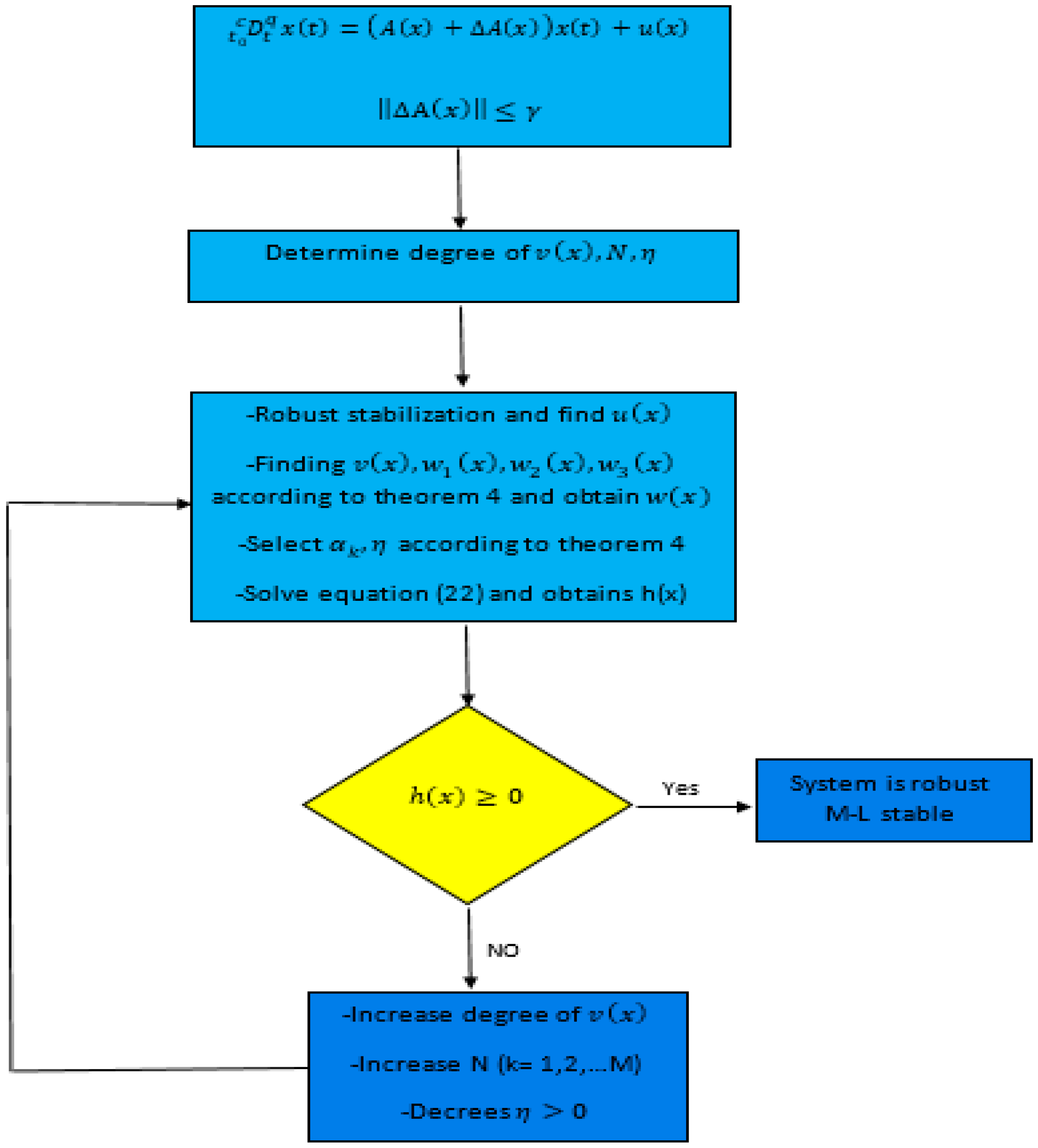
The flowchart of the proposed method is drawn in Figure 1.

6. Examples and Simulations

In this section, by giving examples, we show the efficiency of the methods expressed in Theorems 3–5.

Example 1.

Consider the following PFD equations system

$$\begin{gathered} {}_{t_0}{}^{c}D_t^{0.8}{x}_1\left(t\right)=-x_1-2x_1{x}_2{}^2-2x_2{}^3. \\ {}_{t_0}{}^{c}D_t^{0.8}{x}_2\left(t\right)=-2x_1{}^2{x}_2-2x_2+0.33x_2{}^3. \\ A\left(x\right)=\left[\begin{array}{cc}-1& -2x_1{x}_2-2x_2{}^2\\ -2x_1{x}_2& 0.33x_2{}^2-2\end{array}\right], \Delta A\left(x\right)=0 \end{gathered}$$

(28)

By using SOSTOOLS we have

$$\begin{array}{cc}\hfill v\left(x\right)=0.40401x_1{}^4& +0.375x_1{}^2{x}_2{}^2+0.866x_1{}^2+0.396x_2{}^3{x}_1-0.026x_1{x}_2\hfill \\ \hfill & +0.473x_2{}^4+0.918x_2{}^2.\hfill \end{array}$$

(29)

The Lyapunov function obtained is degrees four in this example, whereas no quadratic function can be found for the system.

$v\left(x\right)=z^{T}Qz$, where$z^T=\left[x_1{x}_2{x}_1{}^2{x}_1{x}_2{x}_2{}^2\right]$and

$$Q=\left[\begin{array}{ccc}\begin{array}{c}0.8662\\ -0.0134\\ 0.0000\end{array}& \begin{array}{c}-0.0134\\ 0.9180\\ 0.0000\end{array}& \begin{array}{c}\begin{array}{ccc}0.0000& 0.0000& 0.0000\end{array}\\ \begin{array}{ccc}0.0000& 0.0000& 0.0000\end{array}\\ \begin{array}{ccc}0.4016& 0.0000& -0.1046\end{array}\end{array}\\ 0.0000& 0.0000& \begin{array}{ccc}0.000& 0.5843& 0.1981\end{array}\\ 0.0000& 0.0000& \begin{array}{ccc}-0.1046& 0.1981& 0.4737\end{array}\end{array}\right]$$

(30)

According to Theorem 3:

$$\begin{array}{cc}\hfill w_1\left(x\right)=0.246x_1{}^4& +0.22875x_1{}^2{x}_2{}^2+0.571x_1{}^2+0.1702x_2{}^3{x}_1-0.026x_1{x}_2\hfill \\ \hfill & +0.010x_2{}^4+0.605x_2{}^2.\hfill \end{array}$$

(31)

$$\begin{array}{cc}\hfill w_2\left(x\right)=0.741x_1{}^8& +0.695x_1{}^6{x}_2{}^2+1.866x_1{}^6+0.3315x_2{}^3{x}_1{}^5-0.0228x_1{}^5{x}_2\hfill \\ \hfill & +1.575x_2{}^4{x}_1{}^4+1.683x_2{}^2{x}_1{}^4+0.695x_1{}^4{x}_2{}^6+1.866x_1{}^2{x}_2{}^4\hfill \\ \hfill & +0.3315x_2{}^7{x}_1-0.0228x_2{}^5{x}_1+0.875x_2{}^8+1.683x_2{}^6.\hfill \end{array}$$

(32)

$$\begin{array}{cc}\hfill w_3\left(x\right)=-4.77x_1{}^4{x}_2{}^2& -1.606x_1{}^4-5.590x_1^3{x}_2^3+0.053x_1{}^3{x}_2-0.0075x_1{}^2{x}_2^6\hfill \\ \hfill & -5.064x_1^2{x}_2^4-9.38x_1^2{x}_2^2-1.73x_1^2-0.011x_1{x}_2^7\hfill \\ \hfill & -1.935x_1{x}_2^5-6.192x_1{x}_1{x}_2^3+0.0803x_1{x}_1{x}_2^2-0.018x_2^8.\hfill \end{array}$$

(33)

Then $x=0$ is Mittag–Leffler stable.

Figure 2 is drawn for different initial conditions that show the stability of the system (25).

Example 2.

Consider the following PFD system

$$\begin{gathered} {}_{t_0}{}^{c}D_t^{0.8}{x}_1\left(t\right)=-4x_1+2x_1{x}_2{}^2+0.2x_1\sin \left(x_1+2x_2\right). \\ {}_{t_0}{}^{c}D_t^{0.8}{x}_2\left(t\right)=-x_2-2x_1{}^2{x}_2+0.3x_{2}cos{x}_1. \end{gathered}$$

(34)

Thus $A\left(x\right)=\left[\begin{array}{cc}-4& 2x_1{x}_2\\ -2x_1{}^2{x}_2& -1\end{array}\right],\Delta A\left(x\left(t\right)\right)=\left[\begin{array}{cc}0.2\sin \left(x_1+2x_2\right)& 0\\ 0& 0.3\cos x_1\end{array}\right]$ is the uncertainty function and $\left|\right|\Delta A\left(x\right)\left|\right|\le 0.36$. The state response of the system (34) with q = 0.8 demonstrate the instability of the system. According to Equation (26), we obtain polynomial controller $u_1\left(x\right)=2.98x_1+4.0761x_2{}^2{x}_1$ and obtain the condition of Theorem 4 by using SOSTOOLS.

The degree of Lyapunov function is 6 by using $\eta =0.01$, ${\alpha }_1=3.6$ in Equations (21) and (23).

$$\begin{gathered} v\left(x\right)=0.0328x_1^6+0.3831x_1^4{x}_2^2+0.3287x_1^4+1.211x_1^2{x}_2^{4}1.512x_1^2{x}_2^2 \\ +0.9734x_1^2+1.285x_2^6+1.313x_2^4+1.276x_2^2. \end{gathered}$$

(35)

$$\begin{array}{cc}\hfill w_1\left(x\right)=0.001x_1^6& +0.1731x_1^4{x}_2^2+0.0187x_1^4+0.134x_1^2{x}_2^4+0.414x_1^2{x}_2^2\hfill \\ \hfill & +0.253x_1^2+0.175x_2^6+0.115x_2^4+0.575x_2^2.\hfill \end{array}$$

(36)

$$\begin{array}{cc}\hfill w_2\left(x\right)=1.234x_1^6& +2.485x_1^4{x}_2^2+1.52x_1^4+4.314x_1^2{x}_2^4+3.812x_1^2{x}_2^2\hfill \\ \hfill & +0.973x_1^2+1.285x_2^6+1.313x_2^4+3.54x_2^2.\hfill \end{array}$$

(37)

$$\begin{array}{cc}\hfill w_3\left(x\right)=0.24x_1^4{x}_2^2& +0.206x_1^4+0.744x_1^2{x}_2^4+1.01x_1^2{x}_2^2+2.62x_1^2+0.39x_2^4\hfill \\ \hfill & +2.16x_2^2.\hfill \end{array}$$

(38)

$w_1\left(x\right),w_2\left(x\right),w_3\left(x\right)$ are SOS and $h\left(x\right)\ge 0$. Then the closed-loop system (34) is robust M-L stable.

Figure 3 is drawn for different initial conditions that show the stability of the closed-loop system (34).

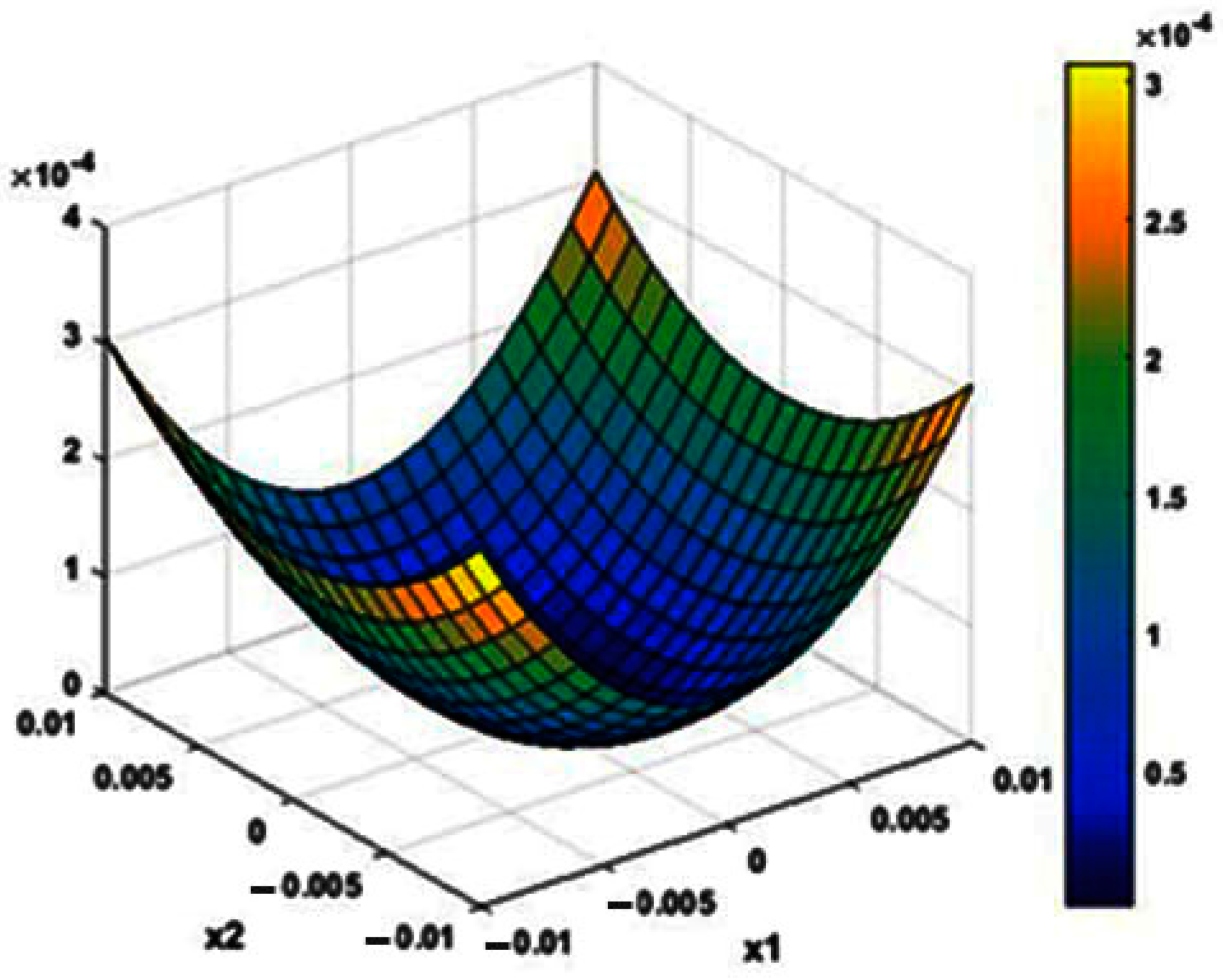
Figure 4 and Figure 5 demonstrate that Equation (25) is valid and its value is also valid for different values of $x_1\left(t\right),x_2\left(t\right)$.

Example 3.

Consider the following PFD equations system

$$\begin{gathered} {}_{t_0}{}^{c}D_t^{0.9}{x}_1\left(t\right)=-2x_1-4x_1{x}_2{}^2+0.3x_1\sin \left(t\right)\sin \left(x_1-x_2\right). \\ {}_{t_0}{}^{c}D_t^{0.9}{x}_2\left(t\right)=-x_2-2x_1{}^2{x}_2+0.4x_2\cos x_1\cos \left(t\right) \end{gathered}$$

(39)

where $\Delta A\left(x\left(t\right),t\right)=\left[\begin{array}{cc}0.3\sin \left(\mathrm{t}\right)\sin \left(x_1-x_2\right)& 0\\ 0& 0.4\cos \left(t\right)\cos x_1\end{array}\right]$is the uncertainty function and $\left|\right|\Delta A\left(x,t\right)\left|\right|\le 0.5$.

The state response of the system (39) with q = 0.9 demonstrates the instability of the system.

According to Equation (26), we obtain a polynomial controller

$$u_1\left(x\right)=-1.85x_1+7.24x_1{x}_2{}^2.$$

(40)

By obtaining $\eta =0.98$, ${\alpha }_1=0.2$, then

$$\begin{array}{cc}\hfill w_1\left(x\right)=0.002x_1^6& +0.218x_1^4{x}_2^2+0.224x_1^4+0.325x_1^2{x}_2^4+0.458x_1^2{x}_2^2\hfill \\ \hfill & +0.281x_1^2+0.021x_1^6+0.321x_1^4{x}_2^2+0.236x_1^4+0.352x_1^2{x}_2^4\hfill \\ \hfill & +0.432x_2^2+0.621x_1^2+0.321x_2^6+0.123x_2^4+0.218x_2^2.\hfill \end{array}$$

(41)

$$\begin{array}{cc}\hfill w_2\left(x\right)=3.78738x_1^6{x}_2^2& +0.9357x_1^6+14.481x_1^4{x}_2^4+14.200x_1^2{x}_2^2+2.79x_1^2\hfill \\ \hfill & +14.52x_1^4{x}_2^2+3.4918x_1^4+13.8665x_1^2{x}_2^6+14.10980x_1^2{x}_2^4\hfill \\ \hfill & +3.5244x_2^6+0.89449x_2^4+2.2365x_2^2.\hfill \end{array}$$

(42)

$$\begin{array}{cc}\hfill w_3\left(x\right)=0.98x_1^6{x}_2^2& +1.77x_1^6+2.985x_1^4{x}_2^4+7.2x_1^4{x}_2^2+6.633x_1^4+3.64x_1^2{x}_2^6\hfill \\ \hfill & +7.9x_1^2{x}_2^4-7.864x_1^2{x}_2^2+5.319x_1^2+2.467x_2^6+0.626x_2^4\hfill \\ \hfill & -1.656x_2^2.\hfill \end{array}$$

(43)

The degree of Lyapunov function is 6 by using the conditions of Theorem 4.

$$\begin{array}{cc}\hfill v\left(x\right)=0.007798x_1^6& +0.479x_1^4{x}_2^2+0.4365x_1^4+0.8522x_1^2{x}_2^4+0.6879x_1^2{x}_2^2\hfill \\ \hfill & +0.741x_1^2+0.07798x_1^6+0.479x_1^4{x}_2^2+0.4365x_1^4\hfill \\ \hfill & +0.8522x_1^2{x}_2^4+0.67879x_1^2{x}_2^2+0.7x_1^2+0.5874x_2^6\hfill \\ \hfill & +0.2236x_2^4+1.118x_2^2.\hfill \end{array}$$

(44)

Figure 6 is drawn for different initial conditions that show the stability of the closed-loop system (39).

Figure 7 and Figure 8 demonstrate that Equation (25) is valid and its value is also valid for different values of x₁(t), x₂(t).

7. Advantages of the Proposed Approach and Suggestions for Future Research

In this paper, the method of PFD systems was highlighted. The main advantages of the proposed method are as follows.

First, the convex Lyapunov methods in the literature such as [19,21] are complicated and are not able to handle the stability and control performances. Second, although the results of some studies (e.g., [9,14,15]) are obtained based on the LMI approach, many design problems cannot be represented by the LMI inequality. This paper focused on the sum of squares approach for finding a Lyapunov candidate function for PFD systems with uncertainty.

Finally, compared with the existing studies on the stability analysis of nonlinear fractional differential systems (e.g., [14]), the results use the Lyapunov quadratic function in the stability analysis. In this paper, higher-order Lyapunov functions were used in the stability analysis of FDE systems based on the sum of squares approach. Following this, by working on PFD fuzzy systems, the stability analysis and stabilization of these systems can be obtained.

8. Conclusions

Finding a Lyapunov candidate function is difficult considering the previous methods. In this paper, the stability and stabilization of PFD systems are presently based on the Lyapunov candidate function. This method can provide the Lyapunov candidate function with a degree higher than two. Therefore, they cannot be solved with LMI techniques. Accordingly, the SOS method is used for solving. For this reason, the system (7) is Mittag–Leffler stable if the Lyapunov functional can satisfy the conditions of Theorem 3. Following this, the sufficient condition of a robust stability system (17) is expressed in Theorem (4). Finally, the polynomial Lyapunov approach is proposed using SOSTOOLS for fractional systems. This method can provide an efficient way for analyzing the stability of an uncertain polynomial fractional system.

References

- Ortigueira, M.D. Fractional Calculus for Scientists and Engineers; Springer Science & Business Media: Berlin/Heidelberg, Germany, 2011; Volume 84. [Google Scholar]
- Caponetto, R. Fractional Order Systems: Modeling and Control Applications; World Scientific: Singapore, 2010; Volume 72. [Google Scholar]
- Mainardi, F. Fractional Calculus and Waves in Linear Viscoelasticity: An Introduction to Mathematical Models; World Scientific: Singapore, 2010. [Google Scholar]
- Idiou, D.; Charef, A.; Djouambi, A. Linear fractional order system identification using adjustable fractional order differentiator. IET Signal Process. 2013, 8, 398–409. [Google Scholar] [CrossRef]
- Balochian, S.; Sedigh, A.K.; Zare, A. Variable structure control of linear time invariant fractional order systems using a finite number of state feedback law. Commun. Nonlinear Sci. Numer. Simul. 2011, 16, 1433–1442. [Google Scholar] [CrossRef]
- Ding, S.; Wang, Z.; Rong, N.; Zhang, H. Exponential stabilization of memristive neural networks via saturating sampled-data control. IEEE Trans. Cybern. 2017, 47, 3027–3039. [Google Scholar] [CrossRef] [PubMed]
- Mayo-Maldonado, J.C.; Fernandez-Anaya, G.; Ruiz-Martinez, O.F. Stability of conformable linear differential systems: A behavioral framework with applications in fractional-order control. IET Control. Theory Appl. 2020, 14, 2900–2913. [Google Scholar] [CrossRef]
- Zhang, R.; Tian, G.; Yang, S.; Cao, H. Stability analysis of a class of fractional order nonlinear systems with order lying in (0, 2). ISA Trans. 2015, 56, 102–110. [Google Scholar] [CrossRef]
- Zhao, Y.; Wang, Y.; Li, H. State feedback control for a class of fractional order nonlinear systems. IEEE/CAA J. Autom. Sin. 2016, 3, 483–488. [Google Scholar]
- Wen, X.-J.; Wu, Z.-M.; Lu, J.-G. Stability analysis of a class of nonlinear fractional-order systems. IEEE Trans. Circuits Syst. II Express Briefs 2008, 55, 1178–1182. [Google Scholar] [CrossRef]
- Chen, L.; Wu, R.; Cheng, Y.; Chen, Y.Q. Delay-dependent and order-dependent stability and stabilization of fractional-order linear systems with time-varying delay. IEEE Trans. Circuits Syst. II Express Briefs 2019, 67, 1064–1068. [Google Scholar] [CrossRef]
- Jiang, P.; Zeng, Z.; Chen, J. On the periodic dynamics of memristor-based neural networks with leakage and time-varying delays. Neurocomputing 2017, 219, 163–173. [Google Scholar] [CrossRef]
- Wen, S.; Zeng, Z.; Huang, T. Exponential stability analysis of memristor-based recurrent neural networks with time-varying delays. Neurocomputing 2012, 97, 233–240. [Google Scholar] [CrossRef]
- Lu, J.-G.; Chen, G. Robust stability and stabilization of fractional-order interval systems: An LMI approach. IEEE Trans. Autom. Control 2009, 54, 1294–1299. [Google Scholar]
- Li, B.; Zhang, X. Observer-based robust control of 0 < α < 1 fractional-order linear uncertain control systems. IET Control. Theory Appl. 2016, 10, 1724–1731. [Google Scholar]
- Lu, J.G.; Chen, Y.Q. Robust Stability and Stabilization of Fractional-Order Interval Systems with the Fractional Order α: The 0 < α < 1 Case. IEEE Trans. Autom. Control. 2009, 55, 152–158. [Google Scholar]
- Zhao, Y.; Wang, Y.; Zhang, X.; Li, H. Feedback stabilisation control design for fractional order non-linear systems in the lower triangular form. IET Control Theory Appl. 2016, 10, 1061–1068. [Google Scholar] [CrossRef]
- Li, Y.; Chen, Y.; Podlubny, I. Stability of fractional-order nonlinear dynamic systems: Lyapunov direct method and generalized Mittag–Leffler stability. Comput. Math. Appl. 2010, 59, 1810–1821. [Google Scholar] [CrossRef] [Green Version]
- Badri, V.; Tavazoei, M.S. Stability analysis of fractional order time-delay systems: Constructing new Lyapunov functions from those of integer order counterparts. IET Control. Theory Appl. 2019, 13, 2476–2481. [Google Scholar] [CrossRef]
- Li, Y.; Chen, Y.; Podlubny, I. Mittag-Leffler stability of fractional order nonlinear dynamic systems. Automatica 2009, 45, 1965–1969. [Google Scholar] [CrossRef]
- Thanh, N.T.; Trinh, H.; Phat, V.N. Stability analysis of fractional differential time-delay equations. IET Control. Theory Appl. 2017, 11, 1006–1015. [Google Scholar] [CrossRef]
- Chen, L.; Chai, Y.; Wu, R.; Yang, J. Stability and stabilization of a class of nonlinear fractional-order systems with Caputo derivative. IEEE Trans. Circuits Syst. II Express Briefs 2012, 59, 602–606. [Google Scholar] [CrossRef]
- Xiao, Q.; Zeng, Z. Lagrange stability for T–S fuzzy memristive neural networks with time-varying delays on time scales. IEEE Trans. Fuzzy Syst. 2017, 26, 1091–1103. [Google Scholar] [CrossRef]
- Bakule, L. Decentralized control: An overview. Annu. Rev. Control 2008, 32, 87–98. [Google Scholar] [CrossRef]
Figure 1.
The proposed method.
Figure 2.
Phase portrait of for PFDE nonlinear system (28).
Figure 3.
Phase portrait of x1(t), x2(t) for PFDE nonlinear system (34).
Figure 4.
Surface h(x) for large range of x1(t), x2(t) and check the condition h(x) > 0 for stability of nonlinear system (34).
Figure 5.
Surface h(x) for small range of x1(t), x2(t) and check the condition h(x) > 0 for stability of nonlinear system (34).
Figure 6.
Phase portrait of x1(t), x2(t) for nonlinear time-variant system (39).
Figure 7.
Surface h(x) for small range of x1(t), x2(t) and check the condition h(x) > 0 for stability of nonlinear time-variant system (31).
Figure 8.
Surface h(x) for small range of x1(t), x2(t) and check the condition h(x) > 0 for stability nonlinear time-variant system (39).
Publisher’s Note: MDPI stays neutral with regard to jurisdictional claims in published maps and institutional affiliations. |
© 2022 by the authors. Licensee MDPI, Basel, Switzerland. This article is an open access article distributed under the terms and conditions of the Creative Commons Attribution (CC BY) license (https://creativecommons.org/licenses/by/4.0/).
Share and Cite
MDPI and ACS Style
Yaghoubi, H.; Zare, A.; Alizadehsani, R. Analysis and Design of Robust Controller for Polynomial Fractional Differential Systems Using Sum of Squares. Axioms 2022, 11, 623. https://0-doi-org.brum.beds.ac.uk/10.3390/axioms11110623
AMA Style
Yaghoubi H, Zare A, Alizadehsani R. Analysis and Design of Robust Controller for Polynomial Fractional Differential Systems Using Sum of Squares. Axioms. 2022; 11(11):623. https://0-doi-org.brum.beds.ac.uk/10.3390/axioms11110623
Chicago/Turabian StyleYaghoubi, Hassan, Assef Zare, and Roohallah Alizadehsani. 2022. "Analysis and Design of Robust Controller for Polynomial Fractional Differential Systems Using Sum of Squares" Axioms 11, no. 11: 623. https://0-doi-org.brum.beds.ac.uk/10.3390/axioms11110623
Note that from the first issue of 2016, this journal uses article numbers instead of page numbers. See further details here.