A Switching Strategy for Stabilization of Discrete-Time Switched Positive Time-Varying Delay Systems with All Modes Being Unstable and Application to Uncertain Data

Abstract

The stability problem of switched systems plays an essential role in the study of long-term behavior. In fact, systems containing both time delay and uncertainty terms may lead to performance degradation of those systems. Therefore, we are interested in the robust stability for discrete-time switched positive time-varying delay systems with interval uncertainties in the case of all modes being unstable. Based on the proposed time-scheduled multiple co-positive Lyapunov–Krasovskii functional of each mode, new sufficient conditions for the global uniform asymptotic stability of the systems are derived. An effective time-dependent switching law utilized in this work is mode-dependent dwell time. In addition, the robust stability criteria in an asymptotic sense are formulated for the systems without time-varying delay. Compared with the existing related works, our results are less conservative and more general than some previous research. Finally, two numerical examples are provided to illustrate the effectiveness and correctness of the developed theoretical results.

1. Introduction

A crucial class of hybrid systems is switched systems which comprise a family of continuous-time modes and a specific rule that controls the switching among them [1]. The applications of switched systems generally occur in many areas, such as robot control systems, electronic circuits and networked control systems. Remarkably, the networked switched systems, which are a combination of the network and switched systems, are becoming popular in the control community. Recently, prominent results can be found in [2,3]. Moreover, switched systems are applied in the development of a switching Kalman Filter structure for sensorless control in a camless engine motor application [4]. However, one of the important topics for discussing switched systems is concerned with their stability. The Lyapunov theory is a vital tool for stability analysis in switched systems. For instance, in [5], the stability problem for the linear switched impulsive systems in Hilbert space has been analyzed via the direct Lyapunov and comparison methods. Slynko et al. [6] proposed an approach to constructing a Lyapunov function (LF) for the stability investigation of a linear large-scale periodic system with possibly unstable subsystems. Chen et al. [7] studied the derivation and improvement of control-oriented compartmental models of the COVID-19 pandemic and design methods from the field of Lyapunov theory guaranteeing the stability of the controlled system. There are two main issues concerning studying the stability of switched systems. One is the characteristic of each mode. Namely, the switched systems may consist of all unstable modes or contain both stable and unstable modes. For the case when partial modes are stable, the stable modes were activated as long as possible to remunerate for the state divergence made by unstable modes. On the other hand, when all modes are unstable, the above idea might be impracticable because of the absence of a stable factor to offset the divergent behavior. Secondly, a switching law plays an essential role in system behavior. It has been mentioned in [8] that a switched system can achieve robust stability (RS) by utilizing suitable switching laws though all modes are unstable. The powerful methodologies for stabilizing switched systems are time-dependent and state-dependent switchings. Nevertheless, in order to stabilize the switched systems with all unstable modes (AUMs), the problem of designing proper switching law, especially the time-dependent switching law, is very interesting and challenging for us in this article.

Several physical engineering and practical systems often contain the term time delay either in system states or control inputs [9]. However, the existence of the time delay could significantly impact system performance degradation [10,11]. Thus, stability analysis of switched systems with time delay has attracted the interest of various scholars. Another factor that may destroy the stability of system dynamics is the presence of the term uncertainty, which refers to the errors between actual and estimated data in the measurement processes and system simulation. There are numerous results on the RS of switched systems, including uncertainties; for example, discrete-time switched systems [12], discrete-time switched positive systems (SPSs) [13], continuous-time SPSs [14,15], switched positive T-S fuzzy systems [16] and stochastic discrete-time switched systems [17,18]. Hence, in this paper, we investigate the robust asymptotic stability (RAS) of a discrete-time switched linear system with time-varying delay (TVD) and uncertainty terms in the form of

$$\begin{array}{c}\hfill \left\{\begin{array}{c}x(k+1)=A_{\sigma \left(k\right)}x\left(k\right)+D_{\sigma \left(k\right)}x(k-d\left(k\right)),\hfill \\ x(k_0+\zeta )=\phi \left(\zeta \right),\zeta =-\widehat{d},-\widehat{d}+1,\dots ,-1,0,\hfill \end{array}\right.\end{array}$$

(1)

where $x\left(k\right)\in {\mathbb{R}}^n$. A switching signal $\sigma \left(k\right)$ is a piecewise constant function specifying at each time instant k. Namely, $\sigma \left(k\right)=i\in \underline{N}=\{1,2,\dots ,N\}$ for $k\in [k_m,k_{m+1})$, where N is the number of modes or subsystems of system (1) and the switching moments are presented by the sequence $k_0<k_1<k_2<\cdots <k_m<k_{m+1}<\cdots <+\infty$. As mentioned in [19,20], the constant system matrices $A_i$ and $D_i$ are supposed to be interval uncertainties (IUs) which can be stated as $A_i\in [{\underline{A}}_i,{\overline{A}}_i]$ and $D_i\in [{\underline{D}}_i,{\overline{D}}_i]$, where ${\underline{A}}_i,{\underline{D}}_i,{\overline{A}}_i,{\overline{D}}_i$ are the given constant system matrices for all $i\in \underline{N}$. $d\left(k\right)$ is the TVD satisfying $d_1\le d\left(k\right)\le d_2$, where $d_1,d_2$ are known positive integers and $\widehat{d}=\max \{d_1,d_2\}$. In addition, $\phi (·):\{-\widehat{d},-\widehat{d}+1,\dots ,-1,0\}\to {\mathbb{R}}^n$ is a given initial state with ${\parallel \phi \parallel }_{\widehat{d}}={\max }_{\zeta \in \{-\widehat{d},-\widehat{d}+1,\dots ,-1,0\}}{\parallel \phi \left(\zeta \right)\parallel }_2$.

On the other hand, SPSs, which concentrate only on the trajectories generated under positivity constraints, can be discovered in various applications such as positive circuit model [21,22], compartmental model [23], water-quality model [24], congestion control [25], network communication [20], formation flying [26], viral mutation [27] and so on. Therefore, SPSs have attracted considerable attention in the past decade. In [20], Feng et al. manipulated the stability and RS problems for linear SPSs with AUMs and IUs. Next, Zhang and Sun [26] examined the practical exponential stability (ES) of discrete-time linear SPSs with impulse and AUMs. Moreover, An et al. [28] investigated the robust exponential stabilization of SPSs with uncertainties based on the assumption that none of the individual modes is stabilizable. From the results in [20,26,28], it should be observed that the existence of the TVD was not taken into account in the systems. Furthermore, there are beneficial results about switched positive time-varying delay systems (SPTVDSs) in cases in which all modes are unstable, reported briefly in the following. In [29], Liu et al. employed the multiple discretized co-positive Lyapunov–Krasovskii functional (MDCPLKF) and dwell time (DT) switching to derive the delay-dependent sufficient criteria (DDSC) of the continuous-time and discrete-time SPTVDSs with AUMs. Later, a sufficient criterion ensuring the global uniform ES of the continuous-time SPTVDSs with AUMs by using the time-scheduled multiple co-positive Lyapunov–Krasovskii functional (TSMCPLKF) method and fast average dwell time (FADT) switching was obtained in [30]. However, among these studies, the IUs have been ignored. Meanwhile, Rojsiraphisal et al. [31] dealt with the RS problem by means of the TSMCPLKF tactic and mode-dependent dwell time (MDDT) switching strategy to guarantee the global uniform asymptotic stability of the continuous-time SPTVDSs including both IUs and AUMs. More recently, Mouktonglang and Yimnet [32] analyzed the global stability problem of SPTVDSs with IUs and AUMs by utilizing FADT switching.

Motivated by the considerations mentioned above, we aim to study the RAS of system (1) with AUMs by applying an appropriate time-dependent switching mechanism. The main contributions of this article are summarized in the following.

(1)

The studied system is more general than numerous existing results since most researchers disregarded the existence and effects of TVD and IUs. In addition, all modes of the studied system are unstable. These factors influence the system’s dynamic behavior and stability.

(2)

Different from the discretized co-positive Lyapunov function (DCPLF) utilized in [20] and the MDCPLKF used in [29], our TSMCPLKF is constructed to analyze the global uniform asymptotic stability of system (1) with AUMs.

(3)

Our work concentrates on designing a suitable switching signal to guarantee the system’s stability, whose modes are all unstable. The applied switching strategy is MDDT which can compensate for the growth of the Lyapunov functional corresponding to each unstable mode. MDDT is different from DT in [29,33] since every mode of the system has its own DT. Namely, MDDT is not the DT of the entire switched system, but it is the DT of the activated ith mode. Therefore, it is worth noting that the MDDT switching rule is less conservative and more applicable in practice than the DT switching rule.

(4)

Under the constraint of a pair of lower and upper bounds for the MDDT switching rule and the TSMCPLKF method, novel DDSC for the RAS of system (1) with AUMs are derived.

2. System Descriptions and Preliminaries

First, we introduce several notations defined throughout this article. ${\mathbb{N}}_0$ and $\mathbb{N}$ are the sets of non-negative integers and positive integers, respectively. Matrix A is called non-negative if all entries are non-negative and denoted by $A⪰0$. The notation $\upsilon ⪰0(\upsilon \succ 0)$ represents a non-negative (positive) vector; namely, all components of $\upsilon$ are non-negative (positive) for vector $\upsilon \in {\mathbb{R}}^n$. $\underline{\omega }\left(\upsilon \right)$ symbolizes the minimal elements of $\upsilon \in {\mathbb{R}}^n$. Furthermore, the floor function $\lfloor x\rfloor =\max \{n\in \mathbb{Z}|n\le x,x\in \mathbb{R}\}$.

Next, we propose the following definitions and lemma that will be used in this paper.

Definition 1 

([29]). System (1) is said to be positive if its states satisfy $x\left(k\right)⪰0,k\in {\mathbb{N}}_0$ for any initial condition $\phi \left(\zeta \right)⪰0,\zeta =-\widehat{d},-\widehat{d}+1,\dots ,-1,0$ and switching signal $\sigma \left(k\right)$.

Lemma 1 

([29]). System (1) is positive if and only if $\forall i\in \underline{N},A_i⪰0$ and $D_i⪰0$.

Definition 2 

([29,33]). System (1) with switching signal $\sigma \left(k\right)$ is said to be:

(1) 

Uniformly stable (US) with respect to $\sigma \left(k\right)$ if $\forall ϵ>0,\exists \delta \left(ϵ\right)>0$ such that ${\parallel x\left(k\right)\parallel }_2<ϵ,\forall k\in [k_0,+\infty )$ whenever ${\parallel \phi \parallel }_{\widehat{d}}<\delta$;

(2) 

Globally uniformly stable (GUS) with respect to $\sigma \left(k\right)$ if $\forall \delta >0$, we have ${\parallel x\left(k\right)\parallel }_2<ϵ,\forall k\in [k_0,+\infty )$;

(3) 

Globally uniformly asymptotically stable (GUAS) with respect to $\sigma \left(k\right)$ if it is GUS and satisfies ${\lim }_{k\to +\infty }x\left(k\right)=0$.

Definition 3 

([16,20]). For the length between successive switching moments during which the ith mode of system (1) is activated, if there exists a constant ${\tau }_{i,m}>0$ such that ${\tau }_{i,m}=k_{m+1}-k_m$ holds for any $i\in \underline{N},m\in {\mathbb{N}}_0$, then the constant ${\tau }_{i,m}$ is called the MDDT of system (1).

Remark 1. 

The MDDT introduced in Definition 3 is different from DT in [29,33] since every mode of system (1) has its own DT. Namely, ${\tau }_{i,m}$ is not the DT of the entire system (1), but it is the DT of the ith mode.

As mentioned in [20], too small or too large DT switching would make system (1) unstable with respect to $\sigma \left(k\right)$. Therefore, the definition of a pair of lower and upper bounds for the MDDT switching law is given as follows:

Definition 4 

([20]). The MDDT switching rule is confined by a pair of lower and upper bounds to guarantee the robust asymptotic stability; namely, ${\tau }_{i,m}\in [{\tau }_{i,min},{\tau }_{i,max}],$ where ${\tau }_{i,min}={\inf }_{m\in {\mathbb{N}}_0}{\tau }_{i,m},{\tau }_{i,max}={\sup }_{m\in {\mathbb{N}}_0}{\tau }_{i,m},0<{\tau }_{i,min}\le {\tau }_{i,max},i\in \underline{N},m\in {\mathbb{N}}_0$. Furthermore, the set of all switching strategies with MDDT ${\tau }_{i,m}\in [{\tau }_{i,min},{\tau }_{i,max}],i\in \underline{N},m\in {\mathbb{N}}_0$ is denoted by the symbol ${\Omega }_{[{\tau }_{i,min},{\tau }_{i,max}]}$.

The central concept of the RAS for system (1) with IUs and AUMs developed from the results in [29,33]. However, we generalize the concept utilized in both references by using the discretized Lyapunov function (DLF) method to establish the suitable TSMCPLKF for our system (1) and applying the MDDT strategy to stabilize our system (1) with AUMs. The detail of the construction of our TSMCPLKF is described in the main theorem and remark. The basic idea of stability analysis for our system (1) is given briefly in the following. When the TSMCPLKF $V_i\left(k\right)$ for each mode of system (1) is constructed, we consider $V_i(k+1)$ along the trajectories of system (1), $k\in [k_m,k_{m+1}),m\in {\mathbb{N}}_0$. Then, we can derive $V_i\left(k\right)<{\gamma }_i^{k-k_m}{V}_i\left(k_m\right),k\in [k_m,k_{m+1}),m\in {\mathbb{N}}_0$ under given scalars ${\gamma }_i>1$ and some sufficient conditions defined specially in the main theorem. We impose that system (1) switches from the jth subsystem to the ith subsystem at the switching instant $k_m$, where $\sigma (k_m-1)=j$ and $\sigma \left(k_m\right)=i,i,j\in \underline{N}$. Next, we can derive $V_i\left(k_m\right)\le {\mu }_i{V}_j(k_m-1)$ under given scalars $0<{\mu }_i<1$, the definition of the discretized vector function and a condition defined specifically in the main theorem. For given values ${\tau }_{j,min}>0,j\in \underline{N}$, if there exist constants ${\tau }_{j,max}\ge {\tau }_{j,min},j\in \underline{N}$ satisfying the MDDT switching rule; that is, $\ln {\mu }_i+{\tau }_{j,max}\ln {\gamma }_j<0,$ for any $i,j\in \underline{N},i\ne j$; this implies ${\mu }_i{\gamma }_j^{{\tau }_{j,max}}<1$, which leads to $V_i\left(k_m\right)<\rho V_j\left(k_{m-1}\right)$ by letting $\rho ={\max }_{i,j\in \underline{N},i\ne j}\left\{{\mu }_i{\gamma }_j^{{\tau }_{j,max}}\right\}$. Obviously, this satisfies $0<\rho <1$ and $V_{\sigma \left(k_m\right)}\left(k_m\right)<\dots <{\rho }^m{V}_{\sigma \left(0\right)}\left(0\right)$. Thus, we can obtain ${\lim }_{m\to +\infty }{V}_{\sigma \left(k_m\right)}\left(k_m\right)=0$, which implies ${\lim }_{m\to +\infty }x\left(k_m\right)=0$. By the fact that the sequence $V_{\sigma \left(k_m\right)}\left(k_m\right),m=0,1,2,\dots$ is strictly decreasing, we obtain ${\lim }_{k\to +\infty }x\left(k\right)=0$. Therefore, system (1) can be proved briefly to be GUAS with respect to switching signal $\sigma \left(k\right)$.

3. Main Results

In this section, we will establish novel DDSC on the positivity and the RAS for system (1) with IUs and AUMs. Because every mode considered in this article is only unstable, we apply the TSMCPLKF method constructed for each mode to solve the stabilization problem by designing the MDDT switching law.

Now, we state the DDSC of system (1) as follows.

Theorem 1. 

Assume that the constant system matrices ${\underline{A}}_i⪰0$ and ${\underline{D}}_i⪰0$ for all $i\in \underline{N}$. For given values $0<{\mu }_i<1,{\gamma }_i>1,{\tau }_{i,min}>0,i\in \underline{N}$ and $L\in \mathbb{N}$, system (1) is positive and GUAS with respect to $\sigma \left(k\right)\in {\Omega }_{[{\tau }_{i,min},{\tau }_{i,max}]}$ if there exist positive vectors ${\upsilon }_{i,q},i\in \underline{N},q\in {\underline{L}}_0$ and constants ${\tau }_{i,max}\ge {\tau }_{i,min},i\in \underline{N}$ satisfying the following conditions:

$$\left({\overline{A}}_i^T+(d_2-d_1+1){\tilde{D}}^T\right){\Phi }_{i,q}+\left({\overline{A}}_i^T+(d_2-d_1+1){\tilde{D}}^T-{\gamma }_i{I}_n\right){\upsilon }_{i,q}\prec 0,$$

(2)

$$\left({\overline{A}}_i^T+(d_2-d_1+1){\tilde{D}}^T\right){\Phi }_{i,q}+\left({\overline{A}}_i^T+(d_2-d_1+1){\tilde{D}}^T-{\gamma }_i{I}_n\right){\upsilon }_{i,q+1}\prec 0,$$

(3)

$${\tilde{D}}^T\left({\Phi }_{i,q}+(1-{\gamma }_i){\upsilon }_{i,q}\right)\prec 0,$$

(4)

$${\tilde{D}}^T\left({\Phi }_{i,q}+(1-{\gamma }_i){\upsilon }_{i,q+1}\right)\prec 0,$$

(5)

$$\left({\overline{A}}_i^T+(d_2-d_1+1){\tilde{D}}^T-{\gamma }_i{I}_n\right){\upsilon }_{i,L}\prec 0,$$

(6)

$${\upsilon }_{i,0}-{\mu }_i{\upsilon }_{j,L}⪯0,$$

(7)

$$\ln {\mu }_i+{\tau }_{j,max}\ln {\gamma }_j<0,$$

(8)

for any $q=0,1,\dots ,L-1$ and for any $i,j\in \underline{N},i\ne j$, where

$${\Phi }_{i,q}={\displaystyle \frac{{\upsilon }_{i,q+1}-{\upsilon }_{i,q}}{{\hslash }_i}},$$

(9)

$${\hslash }_i=\lfloor \frac{{\tau }_{i,min}}{L}\rfloor ,\tilde{D}=\left({\overline{d}}_{kl}\right)\in {\mathbb{R}}^{n\times n},{\overline{d}}_{kl}=\underset{i\in \underline{N}}{\max }\left\{{\overline{D}}_i^{\left(kl\right)}\right\},$$

and ${\overline{D}}_i^{\left(kl\right)}$ is the kth row and lth column element of system matrices ${\overline{D}}_i,i\in \underline{N}$.

Proof. 

The proof is divided into two parts. In part 1, we will prove that system (1) is positive. In part 2, we will show that system (1) is GUAS with respect to $\sigma \left(k\right)\in {\Omega }_{[{\tau }_{i,min},{\tau }_{i,max}]}$.

Part 1:

The positivity of system (1) is proved as follows.

Obviously, this implies that $A_i⪰0$ and $D_i⪰0$ for all $i\in \underline{N}$ by using assumption. According to Lemma 1, system (1) is positive.

Part 2:

The global uniform asymptotic stability of system (1) is shown as follows.

For given $k\in \mathbb{N}$, we suppose that $k\in [k_m,k_{m+1})=[k_m,k_m+{\tau }_{i,min})\cup [k_m+{\tau }_{i,min},k_{m+1}),$$m\in {\mathbb{N}}_0,$ and ${\tau }_{i,min},i\in \underline{N}$ defined as in Definition 4. The interval $[k_m,k_m+{\tau }_{i,min})$ is split into L segments with equal length ${\hslash }_i=\lfloor \frac{{\tau }_{i,min}}{L}\rfloor$. We define ${\mathbb{N}}_{m,q}^i=[k_m+q{\hslash }_i,k_m+(q+1){\hslash }_i),q=0,1,\dots ,L-1$ and stipulate that $[k_m,k_m+{\tau }_{i,min})={\bigcup }_{q=0}^{L-1}{\mathbb{N}}_{m,q}^i$.

To prove the RAS of system (1), we define the following TSMCPLKF based on the concept of MDCPLKF used in [29]. For any $i\in \underline{N}$,

$$V_i(k,x\left(k\right))=x^T\left(k\right){\upsilon }_i\left(k\right)+\sum _{h=k-d\left(k\right)}^{k-1}{x}^T\left(h\right){\tilde{D}}^T{\upsilon }_i\left(k\right)+\sum _{l=-d_2+1}^{-d_1}\sum _{h=k+l}^{k-1}{x}^T\left(h\right){\tilde{D}}^T{\upsilon }_i\left(k\right),$$

(10)

where the vector function:

$$\begin{array}{cc}\hfill {\upsilon }_i\left(k\right)=& {\upsilon }_i(k_m+q{\hslash }_i+r_i)\hfill \\ \hfill =& \left\{\begin{array}{c}\left(1-\frac{r_i}{{\hslash }_i}\right){\upsilon }_{i,q}+\frac{r_i}{{\hslash }_i}{\upsilon }_{i,q+1},k\in {\mathbb{N}}_{m,q}^i,r_i=0,1,\dots ,{\hslash }_i,q=0,1,\dots ,L-1,\hfill \\ {\upsilon }_{i,L},k\in [k_m+{\tau }_{i,min},k_{m+1}),\hfill \end{array}\right.\hfill \end{array}$$

(11)

and ${\upsilon }_{i,q}$ are positive vectors for $i\in \underline{N},q\in {\underline{L}}_0=\{0,1,2,\dots ,L\}$.

When $k\in {\mathbb{N}}_{m,q}^i,$ it can be seen that

$$\begin{array}{cc}\hfill {\upsilon }_i(k+1)-{\upsilon }_i\left(k\right)=& {\upsilon }_i(k_m+q{\hslash }_i+r_i+1)-{\upsilon }_i(k_m+q{\hslash }_i+r_i)\hfill \\ \hfill =& \left[\left(1-\frac{(r_i+1)}{{\hslash }_i}\right){\upsilon }_{i,q}+\frac{(r_i+1)}{{\hslash }_i}{\upsilon }_{i,q+1}\right]-\left[\left(1-\frac{r_i}{{\hslash }_i}\right){\upsilon }_{i,q}+\frac{r_i}{{\hslash }_i}{\upsilon }_{i,q+1}\right].\hfill \end{array}$$

That is,

$${\upsilon }_i(k+1)-{\upsilon }_i\left(k\right)={\Phi }_{i,q},$$

where ${\Phi }_{i,q}$ is defined as in Equation (9).

Considering $V_i(k+1,x(k+1))$ in Equation (10) along the trajectories of system (1), we obtain

$$\begin{array}{cc}\hfill V_i(k+1,x(k+1))=& x^T\left(k\right)A_i^T{\upsilon }_i(k+1)+x^T(k-d\left(k\right))D_i^T{\upsilon }_i(k+1)\hfill \\ \hfill & +\sum _{h=k+1-d(k+1)}^k{x}^T\left(h\right){\tilde{D}}^T{\upsilon }_i(k+1)+\sum _{l=-d_2+1}^{-d_1}\sum _{h=k+1+l}^k{x}^T\left(h\right){\tilde{D}}^T{\upsilon }_i(k+1),\hfill \end{array}$$

then

$$\begin{array}{cc}\hfill V_i(k+1,x(k+1))\le & x^T\left(k\right){\overline{A}}_i^T{\upsilon }_i(k+1)+x^T(k-d\left(k\right)){\overline{D}}_i^T{\upsilon }_i(k+1)\hfill \\ \hfill & +\sum _{h=k+1-d(k+1)}^k{x}^T\left(h\right){\tilde{D}}^T{\upsilon }_i(k+1)+\sum _{l=-d_2+1}^{-d_1}\sum _{h=k+1+l}^k{x}^T\left(h\right){\tilde{D}}^T{\upsilon }_i(k+1).\hfill \end{array}$$

It immediately follows that

$$\begin{array}{cc}\hfill V_i(k+1,x(k+1))-& {\gamma }_i{V}_i(k,x\left(k\right))\hfill \\ \hfill \le & x^T\left(k\right){\overline{A}}_i^T{\upsilon }_i(k+1)+x^T(k-d\left(k\right)){\overline{D}}_i^T{\upsilon }_i(k+1)\hfill \\ \hfill & +\sum _{h=k+1-d(k+1)}^k{x}^T\left(h\right){\tilde{D}}^T{\upsilon }_i(k+1)+\sum _{l=-d_2+1}^{-d_1}\sum _{h=k+1+l}^k{x}^T\left(h\right){\tilde{D}}^T{\upsilon }_i(k+1)\hfill \\ \hfill & -{\gamma }_i{x}^T\left(k\right){\upsilon }_i\left(k\right)-{\gamma }_i\sum _{h=k-d\left(k\right)}^{k-1}{x}^T\left(h\right){\tilde{D}}^T{\upsilon }_i\left(k\right)-{\gamma }_i\sum _{l=-d_2+1}^{-d_1}\sum _{h=k+l}^{k-1}{x}^T\left(h\right){\tilde{D}}^T{\upsilon }_i\left(k\right).\hfill \end{array}$$

By the fact that ${\overline{D}}_i⪯\tilde{D}$ for all $i\in \underline{N}$, it can be obtained that

$$\begin{array}{cc}\hfill V_i(k+1,x(k+1))-& {\gamma }_i{V}_i(k,x\left(k\right))\hfill \\ \hfill \le & x^T\left(k\right){\overline{A}}_i^T{\upsilon }_i(k+1)+x^T(k-d\left(k\right)){\tilde{D}}^T{\upsilon }_i(k+1)\hfill \\ \hfill & +{\displaystyle \sum _{h=k-d_2+1}^{k-1}}{x}^T\left(h\right){\tilde{D}}^T{\upsilon }_i(k+1)+x^T\left(k\right){\tilde{D}}^T{\upsilon }_i(k+1)-{\gamma }_i{x}^T\left(k\right){\upsilon }_i\left(k\right)\hfill \\ \hfill & -{\gamma }_i{\displaystyle \sum _{h=k-d_1+1}^{k-1}}{x}^T\left(h\right){\tilde{D}}^T{\upsilon }_i\left(k\right)-{\gamma }_i{x}^T(k-d\left(k\right)){\tilde{D}}^T{\upsilon }_i\left(k\right)\hfill \\ \hfill & +{\displaystyle \sum _{l=-d_2+1}^{-d_1}\sum _{h=k+1+l}^{k-1}}{x}^T\left(h\right){\tilde{D}}^T{\upsilon }_i(k+1)+{\displaystyle \sum _{l=-d_2+1}^{-d_1}}{x}^T\left(k\right){\tilde{D}}^T{\upsilon }_i(k+1)\hfill \\ \hfill & -{\gamma }_i{\displaystyle \sum _{l=-d_2+1}^{-d_1}\sum _{h=k+1+l}^{k-1}}{x}^T\left(h\right){\tilde{D}}^T{\upsilon }_i\left(k\right)-{\gamma }_i{\displaystyle \sum _{l=-d_2+1}^{-d_1}}{x}^T(k+l){\tilde{D}}^T{\upsilon }_i\left(k\right).\hfill \end{array}$$

(12)

Then, we have noticed that

$$\sum _{l=-d_2+1}^{-d_1}{x}^T\left(k\right){\tilde{D}}^T{\upsilon }_i(k+1)=\left(d_2-d_1\right)x^T\left(k\right){\tilde{D}}^T{\upsilon }_i(k+1),$$

and

$${\gamma }_i\sum _{l=-d_2+1}^{-d_1}{x}^T(k+l){\tilde{D}}^T{\upsilon }_i\left(k\right)={\gamma }_i\sum _{h=k-d_2+1}^{k-d_1}{x}^T\left(h\right){\tilde{D}}^T{\upsilon }_i\left(k\right),$$

for all $i\in \underline{N}$. Combining these with Equation (12), we have

$$\begin{array}{cc}\hfill V_i(k+1,x(k+1))-& {\gamma }_i{V}_i(k,x\left(k\right))\hfill \\ \hfill \le & x^T\left(k\right)\left[{\overline{A}}_i^T{\upsilon }_i(k+1)+(d_2-d_1+1){\tilde{D}}^T{\upsilon }_i(k+1)-{\gamma }_i{\upsilon }_i\left(k\right)\right]\hfill \\ \hfill & +x^T(k-d\left(k\right)){\tilde{D}}^T\left[{\upsilon }_i(k+1)-{\gamma }_i{\upsilon }_i\left(k\right)\right]\hfill \\ \hfill & +\sum _{h=k-d_2+1}^{k-1}{x}^T\left(h\right){\tilde{D}}^T\left[{\upsilon }_i(k+1)-{\gamma }_i{\upsilon }_i\left(k\right)\right]\hfill \\ \hfill & +\sum _{l=-d_2+1}^{-d_1}\sum _{h=k+1+l}^{k-1}{x}^T\left(h\right){\tilde{D}}^T\left[{\upsilon }_i(k+1)-{\gamma }_i{\upsilon }_i\left(k\right)\right],\hfill \end{array}$$

for any $k\in {\mathbb{N}}_{m,q}^i$ and $i\in \underline{N}$. When $k\in {\mathbb{N}}_{m,q}^i\subset [k_m,k_m+{\tau }_{i,min})$, it can be seen that

$$\begin{array}{cc}\hfill {\overline{A}}_i^T{\upsilon }_i(k+1)& +(d_2-d_1+1){\tilde{D}}^T{\upsilon }_i(k+1)-{\gamma }_i{\upsilon }_i\left(k\right)\hfill \\ \hfill =& \left(1-\frac{r_i}{{\hslash }_i}\right)\left[\left({\overline{A}}_i^T+(d_2-d_1+1){\tilde{D}}^T\right){\Phi }_{i,q}+\left({\overline{A}}_i^T+(d_2-d_1+1){\tilde{D}}^T-{\gamma }_i{I}_n\right){\upsilon }_{i,q}\right]\hfill \\ \hfill & +\frac{r_i}{{\hslash }_i}\left[\left({\overline{A}}_i^T+(d_2-d_1+1){\tilde{D}}^T\right){\Phi }_{i,q}+\left({\overline{A}}_i^T+(d_2-d_1+1){\tilde{D}}^T-{\gamma }_i{I}_n\right){\upsilon }_{i,q+1}\right],\hfill \end{array}$$

and

$$\begin{array}{c}\hfill {\tilde{D}}^T\left[{\upsilon }_i(k+1)-{\gamma }_i{\upsilon }_i\left(k\right)\right]=\left(1-\frac{r_i}{{\hslash }_i}\right)\left[{\tilde{D}}^T\left({\Phi }_{i,q}+(1-{\gamma }_i){\upsilon }_{i,q}\right)\right]+\frac{r_i}{{\hslash }_i}\left[{\tilde{D}}^T\left({\Phi }_{i,q}+(1-{\gamma }_i){\upsilon }_{i,q+1}\right)\right].\end{array}$$

According to conditions (2)–(5),

$$V_i(k+1,x(k+1))-{\gamma }_i{V}_i(k,x\left(k\right))<0,k\in {\mathbb{N}}_{m,q}^i,$$

which implies

$$V_i(k+1,x(k+1))<{\gamma }_i{V}_i(k,x\left(k\right)),k\in \bigcup _{q=0}^{L-1}{\mathbb{N}}_{m,q}^i=[k_m,k_m+{\tau }_{i,min}).$$

(13)

For $k\in [k_m+{\tau }_{i,min},k_{m+1})$,

$${\overline{A}}_i^T{\upsilon }_i(k+1)+(d_2-d_1+1){\tilde{D}}^T{\upsilon }_i(k+1)-{\gamma }_i{\upsilon }_i\left(k\right)=\left({\overline{A}}_i^T+(d_2-d_1+1){\tilde{D}}^T-{\gamma }_i{I}_n\right){\upsilon }_{i,L},$$

and

$${\tilde{D}}^T\left[{\upsilon }_i(k+1)-{\gamma }_i{\upsilon }_i\left(k\right)\right]={\tilde{D}}^T(1-{\gamma }_i){\upsilon }_{i,L}\prec 0.$$

Using condition (6), we obtain

$$V_i(k+1,x(k+1))<{\gamma }_i{V}_i(k,x\left(k\right)),k\in [k_m+{\tau }_{i,min},k_{m+1}).$$

(14)

Applying Equations (13) and (14), we obtain

$$V_i(k+1,x(k+1))<{\gamma }_i{V}_i(k,x\left(k\right)),k\in [k_m,k_{m+1}),m\in {\mathbb{N}}_0.$$

This implies

$$V_i(k,x\left(k\right))<{\gamma }_i^{k-k_m}{V}_i(k_m,x\left(k_m\right)),k\in [k_m,k_{m+1}),m\in {\mathbb{N}}_0.$$

(15)

Utilizing Equations (10), (11) and condition (7), we have

$$V_i(k_m,x\left(k_m\right))\le {\mu }_i{V}_j(k_m-1,x(k_m-1)),k_m-1\in [k_{m-1}+{\tau }_{j,min},k_m),m\in {\mathbb{N}}_0.$$

(16)

Since $[k_{m-1}+{\tau }_{j,min},k_m)\subset [k_{m-1},k_m)$, one can claim from Equation (15) that

$$V_j(k_m-1,x(k_m-1))<{\gamma }_j^{\left(k_m-1\right)-k_{m-1}}{V}_j(k_{m-1},x\left(k_{m-1}\right)),k_m-1\in [k_{m-1},k_m),$$

which implies

$$V_j(k_m-1,x(k_m-1))<{\gamma }_j^{k_m-k_{m-1}}{V}_j(k_{m-1},x\left(k_{m-1}\right)),k_m-1\in [k_{m-1},k_m),m\in {\mathbb{N}}_0.$$

(17)

From Equations (15)–(17), it follows that

$$\begin{array}{cc}\hfill V_{\sigma \left(k_m\right)}(k,x\left(k\right))<& {\gamma }_{\sigma \left(k_m\right)}^{k-k_m}{V}_{\sigma \left(k_m\right)}(k_m,x\left(k_m\right))\hfill \\ \hfill \le & {\gamma }_{\sigma \left(k_m\right)}^{k-k_m}{\mu }_{\sigma \left(k_m\right)}{V}_{\sigma \left(k_{m-1}\right)}(k_m-1,x(k_m-1))\hfill \\ \hfill <& {\mu }_{\sigma \left(k_m\right)}{\gamma }_{\sigma \left(k_m\right)}^{k-k_m}{\gamma }_{\sigma \left(k_{m-1}\right)}^{k_m-k_{m-1}}{V}_{\sigma \left(k_{m-1}\right)}(k_{m-1},x\left(k_{m-1}\right))\hfill \\ \hfill ⋮\\ \hfill <& {\mu }_{\sigma \left(k_m\right)}{\mu }_{\sigma \left(k_{m-1}\right)}\cdots {\mu }_{\sigma \left(k_1\right)}{\gamma }_{\sigma \left(k_m\right)}^{k-k_m}{\gamma }_{\sigma \left(k_{m-1}\right)}^{k_m-k_{m-1}}\cdots {\gamma }_{\sigma \left(k_0\right)}^{k_1-k_0}{V}_{\sigma \left(k_0\right)}(k_0,x\left(k_0\right))\hfill \\ \hfill =& {\gamma }_{\sigma \left(k_m\right)}^{k-k_m}\left({\mu }_{\sigma \left(k_m\right)}{\gamma }_{\sigma \left(k_{m-1}\right)}^{k_m-k_{m-1}}\right)\cdots \left({\mu }_{\sigma \left(k_1\right)}{\gamma }_{\sigma \left(k_0\right)}^{k_1-k_0}\right)V_{\sigma \left(k_0\right)}(k_0,x\left(k_0\right))\hfill \\ \hfill =& {\gamma }_{\sigma \left(k_m\right)}^{k-k_m}\left(\prod _{l=0}^{m-1}{\mu }_{\sigma \left(k_{l+1}\right)}{\gamma }_{\sigma \left(k_l\right)}^{k_{l+1}-k_l}\right)V_{\sigma \left(k_0\right)}(k_0,x\left(k_0\right))\hfill \\ \hfill \le & {\gamma }_{\sigma \left(k_m\right)}^{{\tau }_{\sigma \left(k_m\right),max}}\left(\prod _{l=0}^{m-1}{\mu }_{\sigma \left(k_{l+1}\right)}{\gamma }_{\sigma \left(k_l\right)}^{{\tau }_{\sigma \left(k_l\right),max}}\right)V_{\sigma \left(k_0\right)}(k_0,x\left(k_0\right)).\hfill \end{array}$$

According to condition (8),

$${\mu }_i{\gamma }_j^{{\tau }_{j,max}}<1,$$

(18)

for all $i,j\in \underline{N},i\ne j$. Without loss of generality, we impose that $V_{\sigma \left(k_0\right)}(k_0,x\left(k_0\right))=V_{\sigma \left(0\right)}(0,x\left(0\right))$. Hence, we obtain

$$V_{\sigma \left(k_m\right)}(k,x\left(k\right))<{\gamma }_{\sigma \left(k_m\right)}^{{\tau }_{\sigma \left(k_m\right),max}}{V}_{\sigma \left(0\right)}(0,x\left(0\right)).$$

Moreover, let $\nu ={\max }_{i\in \underline{N}}\left\{{\tau }_{i,max}\right\}$ and $\Gamma ={\max }_{i\in \underline{N}}\left\{{\gamma }_i\right\}$, then

$$V_{\sigma \left(k_m\right)}(k,x\left(k\right))<{\Gamma }^{\nu }{V}_{\sigma \left(0\right)}(0,x\left(0\right)).$$

(19)

From Equations (10) and (11), we can derive

$$\begin{array}{cc}\hfill V_{\sigma \left(0\right)}(0,x\left(0\right))\le & {\parallel x^T\left(0\right)\parallel }_2{\parallel {\upsilon }_{\sigma \left(0\right)}\left(0\right)\parallel }_2+{\displaystyle \sum _{h=-\widehat{d}}^{-1}}\underset{h\in \{-\widehat{d},-\widehat{d}+1,\dots ,-1,0\}}{\max }{\parallel x^T\left(h\right)\parallel }_2{\parallel {\tilde{D}}^T\parallel }_2{\parallel {\upsilon }_{\sigma \left(0\right)}\left(0\right)\parallel }_2\hfill \\ \hfill & +{\displaystyle \sum _{l=-d_2+1}^{-d_1}\sum _{h=l}^{-1}}\underset{h\in \{-\widehat{d},-\widehat{d}+1,\dots ,-1,0\}}{\max }{\parallel x^T\left(h\right)\parallel }_2{\parallel {\tilde{D}}^T\parallel }_2{\parallel {\upsilon }_{\sigma \left(0\right)}\left(0\right)\parallel }_2\hfill \\ \hfill \le & {\parallel x^T\left(0\right)\parallel }_2{\displaystyle \sum _{b\in {\underline{L}}_0}}{\parallel {\upsilon }_{\sigma \left(0\right),b}\parallel }_2+\widehat{d}\underset{h\in \{-\widehat{d},-\widehat{d}+1,\dots ,-1,0\}}{\max }{\parallel x^T\left(h\right)\parallel }_2{\parallel {\tilde{D}}^T\parallel }_2{\displaystyle \sum _{b\in {\underline{L}}_0}}{\parallel {\upsilon }_{\sigma \left(0\right),b}\parallel }_2\hfill \\ \hfill & +\left(\frac{d_2-d_1}{2}\right)\left(d_2+d_1-1\right)\underset{h\in \{-\widehat{d},-\widehat{d}+1,\dots ,-1,0\}}{\max }{\parallel x^T\left(h\right)\parallel }_2{\parallel {\tilde{D}}^T\parallel }_2{\displaystyle \sum _{b\in {\underline{L}}_0}}{\parallel {\upsilon }_{\sigma \left(0\right),b}\parallel }_2\hfill \\ \hfill \le & \left[1+\left(\widehat{d}+\left(\frac{d_2-d_1}{2}\right)\left(d_2+d_1-1\right)\right){\parallel {\tilde{D}}^T\parallel }_2\right]\sqrt{n}{\displaystyle \sum _{b\in {\underline{L}}_0}}{\parallel {\upsilon }_{\sigma \left(0\right),b}\parallel }_2{\parallel \phi \parallel }_{\widehat{d}}.\hfill \end{array}$$

(20)

Furthermore, we have

$$\begin{array}{c}\hfill \varsigma {\parallel x\left(k\right)\parallel }_2\le V_{\sigma \left(k_m\right)}(k,x\left(k\right)),\end{array}$$

(21)

where $\varsigma ={\min }_{(a,b)\in \underline{N}\times {\underline{L}}_0}\left\{\underline{\omega }\left({\upsilon }_{a,b}\right)\right\}$. Substituting Equations (20) and (21) into Equation (19), it can be obtained that

$${\parallel x\left(k\right)\parallel }_2\le \Theta {\Gamma }^{\nu }{\parallel \phi \parallel }_{\widehat{d}},$$

(22)

for all $k\ge 0$, where $\Theta =\frac{1}{\varsigma }\left[1+\left(\widehat{d}+\left(\frac{d_2-d_1}{2}\right)\left(d_2+d_1-1\right)\right){\parallel {\tilde{D}}^T\parallel }_2\right]\sqrt{n}{\sum }_{b\in {\underline{L}}_0}{\parallel {\nu }_{\sigma \left(0\right),b}\parallel }_2$. Then, for any $ϵ>0$, we can choose

$${\parallel \phi \parallel }_{\widehat{d}}<\delta \left(ϵ\right)=\frac{ϵ}{\Theta {\Gamma }^{\nu }}.$$

Therefore,

$${\parallel x\left(k\right)\parallel }_2<ϵ,$$

for all $k\ge 0$. This implies that system (1) is US. Obviously, for any $\delta >0$, we have ${\parallel x\left(k\right)\parallel }_2<ϵ$ for all $k\ge 0$. Hence, system (1) is GUS with respect to $\sigma \left(k\right)\in {\Omega }_{[{\tau }_{i,min},{\tau }_{i,max}]}$.

Next, we will show that ${\lim }_{k\to +\infty }x\left(k\right)=0$. We consider the sequence $V_{\sigma \left(k_m\right)}(k_m,x\left(k_m\right)),$$m\in {\mathbb{N}}_0$. From Equations (16) and (17), we can derive

$$\begin{array}{cc}\hfill V_i(k_m,x\left(k_m\right))<& {\mu }_i{\gamma }_j^{k_m-k_{m-1}}{V}_j(k_{m-1},x\left(k_{m-1}\right))\hfill \\ \hfill <& {\mu }_i{\gamma }_j^{{\tau }_{j,max}}{V}_j(k_{m-1},x\left(k_{m-1}\right)),\hfill \end{array}$$

for all $i,j\in \underline{N},i\ne j$. Let $\rho ={\max }_{i,j\in \underline{N},i\ne j}\left\{{\mu }_i{\gamma }_j^{{\tau }_{j,max}}\right\}$ and from Equation (18), we obtain

$$V_i(k_m,x\left(k_m\right))<\rho V_j(k_{m-1},x\left(k_{m-1}\right)),$$

when $0<\rho <1,m\in {\mathbb{N}}_0$. This implies that the sequence $V_{\sigma \left(k_m\right)}(k_m,x\left(k_m\right)),m\in {\mathbb{N}}_0$ is strictly decreasing and satisfies

$$\begin{array}{cc}\hfill V_{\sigma \left(k_m\right)}(k_m,x\left(k_m\right))<& \rho V_{\sigma \left(k_{m-1}\right)}(k_{m-1},x\left(k_{m-1}\right))\hfill \\ \hfill ⋮\\ \hfill <& {\rho }^m{V}_{\sigma \left(0\right)}(0,x\left(0\right)).\hfill \end{array}$$

Thus, ${\lim }_{m\to +\infty }{V}_{\sigma \left(k_m\right)}(k_m,x\left(k_m\right))=0$. Since ${\upsilon }_{\sigma \left(k_m\right)}\left(k_m\right)={\upsilon }_{\sigma \left(k_m\right),0}$ and by assumption that there exist positive vectors ${\upsilon }_{i,q},i\in \underline{N},q\in {\underline{L}}_0$, it can be seen that

$${\upsilon }_{\sigma \left(k_m\right)}\left(k_m\right)\succ 0.$$

In addition, from the positivity of system (1), we arrive at

$$\underset{m\to +\infty }{\lim }x\left(k_m\right)=0.$$

The proof in the final part that ${\lim }_{k\to +\infty }x\left(k\right)=0$ is similar to that of Theorems 1 and 3 in [20]. Therefore, it is omitted here. By Definition 2, we can conclude that system (1) is GUAS with respect to $\sigma \left(k\right)\in {\Omega }_{[{\tau }_{i,min},{\tau }_{i,max}]}$. □

Remark 2. 

To stabilize system (1) including both IUs and AUMs, the basic idea of a construction of the TSMCPLKF proposed in Equation (10) has been inspired by the results in [29,33]. In [33], the authors employed the DLF method to divide the domain of definition of vector function ${\upsilon }_i\left(k\right),i\in \underline{N}$ defined in Equation (11) into finite smaller regions; the vector function varies linearly in each small region. The detail of the division of the interval domain is described at the beginning of Part 2 of the proof in Theorem 1. Moreover, by Equation (11), the number of discretized positive vectors ${\upsilon }_{i,q},i\in \underline{N},q\in {\underline{L}}_0=\{0,1,2,\dots ,L\}$ is $L+1$ for given $L\in \mathbb{N}$. Nevertheless, if $L=0$, the DLF is reduced to the multiple LF. Because each mode studied in this work is only unstable, the value of the LFs $V_i\left(k\right),i\in \underline{N}$ may increase. However, the increment of $V_i\left(k\right)$ is recompensed and the stabilization of system (1) can be accomplished via the MDDT switching rule, which is designed to reduce the value of $V_i\left(k\right)$ at the switching instants. Namely, for given values $0<{\mu }_i<1,{\gamma }_i>1,{\tau }_{i,min}>0,i\in \underline{N}$, there exist a set of non-negative functions $V_i\left(k\right)$ and constants ${\tau }_{i,max}\ge {\tau }_{i,min},i\in \underline{N}$ such that $V_i(k+1)<{\gamma }_i{V}_i\left(k\right)$, $V_i\left(k_m\right)\le {\mu }_i{V}_j(k_m-1)$, $\ln {\mu }_i+{\tau }_{j,max}\ln {\gamma }_j<0$, for any $i,j\in \underline{N},i\ne j$. The TSMCPLKF in Equation (10) is logically established for all the reasons mentioned above.

Remark 3. 

Different from the DCPLF utilized in [20] and the MDCPLKF used in [29], our TSMCPLKF defined in Equation (10) is constructed specifically for system (1) including both IUs and AUMs. Moreover, the MDDT switching technique is also applied to ensure the global uniform asymptotic stability of the system. Therefore, our theoretical results are less conservative than those of Theorem 3.4 and Theorem 3.6 in [29].

Remark 4. 

Since the considered system (1) is extremely complex, it is interesting to investigate the RAS of the system. From Theorem 1, new sufficient conditions (2)–(8) are derived to guarantee the positivity and global uniform asymptotic stability of system (1). Although these conditions of the main theorem seem to be strong, they were essentially created to deal with the instability problems of this system caused by all modes being unstable and uncertain terms. As can be seen from the proof of the main theorem, the upper bounds of the system matrices ${\overline{A}}_{i}i\in \underline{N}$ and $\tilde{D}$ in conditions (2)–(6) are given to ensure the RAS of the system including the IUs. Novel DDSC (2)–(6) and condition (7) are acquired by using the DLF and vector function methods. Condition (8), which is the MDDT switching rule, is designed to stabilize the overall switched system (1) where every unstable subsystem is triggered. Thus, the sufficient conditions (2)–(8) in the main theorem are necessary. However, this raises the following question: Is it possible to weaken the conditions of the theorem? This interesting question is challenged in the RAS analysis for system (1). This is still an open problem for research in the future.

Remark 5. 

When the discrete-time switched positive linear system did not involve the TVD, sufficient conditions guaranteeing the asymptotic stability of the system were presented in [20]. Thus, our theoretical results given in this article generalize the corresponding results in [20].

When $D_{\sigma \left(k\right)}\equiv 0,\sigma \left(k\right)\in \underline{N}$, system (1) can be reduced into the discrete-time switched linear system without TVD of the form:

$$\begin{array}{c}\hfill \left\{\begin{array}{c}x(k+1)=A_{\sigma \left(k\right)}x\left(k\right),\hfill \\ x\left(k_0\right)=x_0.\hfill \end{array}\right.\end{array}$$

(23)

The constant matrices $A_i,i\in \underline{N}$ and the assumptions of system (23) are similar to system (1). Namely, ${\underline{A}}_i⪰0$, all modes of system (23) are unstable and MDDT ${\tau }_{i,m}\in [{\tau }_{i,min},{\tau }_{i,max}],$ where ${\tau }_{i,min}={\inf }_{m\in {\mathbb{N}}_0}{\tau }_{i,m},{\tau }_{i,max}={\sup }_{m\in {\mathbb{N}}_0}{\tau }_{i,m},0<{\tau }_{i,min}\le {\tau }_{i,max},i\in \underline{N},m\in {\mathbb{N}}_0$.

Remark 6. 

The discrete-time switched linear system without TVD (23) and its system descriptions were studied in [20].

The last result guaranteeing the positivity and the RAS of system (23) is shown in the following:

Corollary 1. 

For given values $0<{\mu }_i<1,{\gamma }_i>1,{\tau }_{i,min}>0,i\in \underline{N}$ and $L\in \mathbb{N}$, system (23) is positive and GUAS with respect to $\sigma \left(k\right)\in {\Omega }_{[{\tau }_{i,min},{\tau }_{i,max}]}$ if there exist positive vectors ${\upsilon }_{i,q},i\in \underline{N},q\in {\underline{L}}_0$ and constants ${\tau }_{i,max}\ge {\tau }_{i,min},i\in \underline{N}$ satisfying the following conditions:

$${\overline{A}}_i^T{\Phi }_{i,q}+\left({\overline{A}}_i^T-{\gamma }_i{I}_n\right){\upsilon }_{i,q}\prec 0,$$

$${\overline{A}}_i^T{\Phi }_{i,q}+\left({\overline{A}}_i^T-{\gamma }_i{I}_n\right){\upsilon }_{i,q+1}\prec 0,$$

$$\left({\overline{A}}_i^T-{\gamma }_i{I}_n\right){\upsilon }_{i,L}\prec 0,$$

$${\upsilon }_{i,0}-{\mu }_i{\upsilon }_{j,L}⪯0,$$

$$\ln {\mu }_i+{\tau }_{j,max}\ln {\gamma }_j<0,$$

for any $q=0,1,\dots ,L-1$ and for any $i,j\in \underline{N},i\ne j$, where ${\Phi }_{i,q}$ is defined as in (9).

Proof. 

Under the same vector function (11) in Theorem 1, this corollary can be proved by using the DCPLF in the form of

$$V_i(k,x\left(k\right))=x^T\left(k\right){\upsilon }_i\left(k\right),$$

for any $i\in \underline{N}$. The proof is very similar to that of Theorem 1. Thus, the rest of the details will be omitted. □

4. Numerical Simulations

In this section, two numerical examples are presented to illustrate the effectiveness of the theoretical analysis proposed in the previous section.

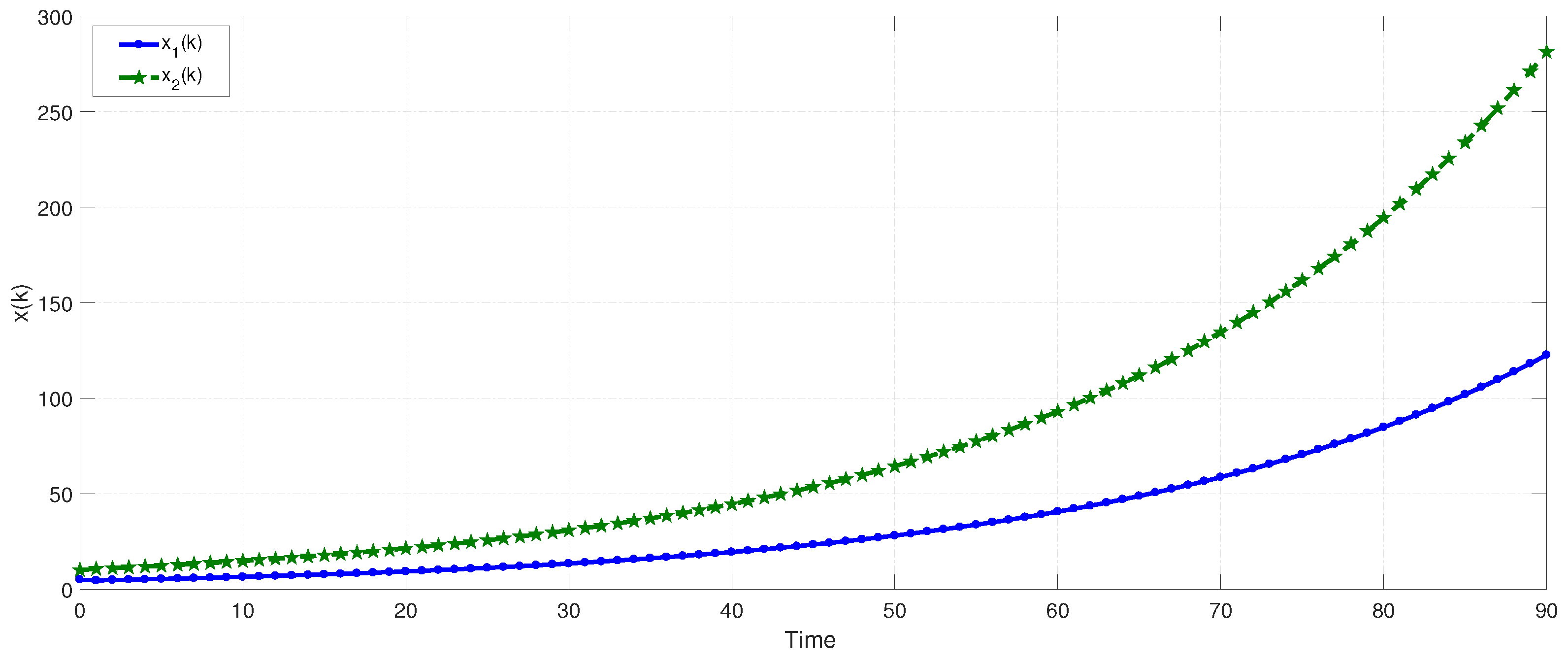
Example 1. In this example, the RAS problem for system (1) consisting of two modes is analyzed. The system matrices are provided as follows:

$${\underline{A}}_1=\left[\begin{array}{cc}0.0049& 0.4470\\ 0.3480& 0.8850\end{array}\right],{\overline{A}}_1=\left[\begin{array}{cc}0.0051& 0.4530\\ 0.3520& 0.8850\end{array}\right],{\underline{D}}_1=\left[\begin{array}{cc}0& 0\\ 0& 0.00002\end{array}\right],{\overline{D}}_1=\left[\begin{array}{cc}0& 0\\ 0& 0.00002\end{array}\right],$$

$${\underline{A}}_2=\left[\begin{array}{cc}1.035& 0.137\\ 0.018& 0.585\end{array}\right],{\overline{A}}_2=\left[\begin{array}{cc}1.045& 0.143\\ 0.022& 0.585\end{array}\right],{\underline{D}}_2=\left[\begin{array}{cc}0.00001& 0\\ 0& 0.00002\end{array}\right],{\overline{D}}_2=\left[\begin{array}{cc}0.00001& 0\\ 0& 0.00002\end{array}\right],$$

and

$$d\left(k\right)=1+{\sin }^2\left(\frac{k\pi }{2}\right).$$

From the given TVD above, we can select $d_1=1,d_2=2$ and $\widehat{d}=2$. It can be obtained that ${\underline{A}}_1⪰0,{\underline{A}}_2⪰0,{\underline{D}}_1⪰0$ and ${\underline{D}}_2⪰0$. Thus, this system is positive by using the assumption and Lemma 1. Then, we carry out the simulation with the initial state generating $\phi \left(\zeta \right)={\left[510\right]}^T,\zeta =-\widehat{d},-\widehat{d}+1,\dots ,-1,0$ and stipulating that the system matrices be

$$A_1=\frac{{\underline{A}}_1+{\overline{A}}_1}{2}=\left[\begin{array}{cc}0.005& 0.450\\ 0.350& 0.885\end{array}\right],D_1=\frac{{\underline{D}}_1+{\overline{D}}_1}{2}=\left[\begin{array}{cc}0& 0\\ 0& 0.00002\end{array}\right],$$

and

$$A_2=\frac{{\underline{A}}_2+{\overline{A}}_2}{2}=\left[\begin{array}{cc}1.040& 0.140\\ 0.020& 0.585\end{array}\right],D_2=\frac{{\underline{D}}_2+{\overline{D}}_2}{2}=\left[\begin{array}{cc}0.00001& 0\\ 0& 0.00002\end{array}\right].$$

The corresponding state responses of two modes are shown in Figure 1 and Figure 2. Obviously, it can be seen from Figure 1 and Figure 2 that two modes are both positive and unstable.

Next, it is obvious that

$$\tilde{D}=\left[\begin{array}{cc}0.00001& 0\\ 0& 0.00002\end{array}\right].$$

Based on conditions (2)–(8) in Theorem 1 and given $L=1,{\mu }_1=0.58,{\gamma }_1=1.34,$ ${\mu }_2=0.55,{\gamma }_2=1.62,{\tau }_{1,min}=2,{\tau }_{2,min}=1$, we obtain the feasible solution:

$${\upsilon }_{1,0}=\left[\begin{array}{c}28.4261\\ 84.8639\end{array}\right],{\upsilon }_{1,1}=\left[\begin{array}{c}66.5702\\ 117.8516\end{array}\right],{\upsilon }_{2,0}=\left[\begin{array}{c}35.8341\\ 64.7436\end{array}\right],{\upsilon }_{2,1}=\left[\begin{array}{c}49.9281\\ 146.6385\end{array}\right],$$

${\tau }_{1,max}=2.001$ and ${\tau }_{2,max}=1.1$. Hence, this system is GUAS under the switching signal $\sigma \left(k\right)\in {\Omega }_{[2,2.001][1,1.1]}$ by Theorem 1. The corresponding switching signal $\sigma \left(k\right)$ and the state responses of the system are presented in Figure 3 and Figure 4, respectively. Therefore, it can be seen that our designed switching signal can ensure the RAS of the system effectively. However, owing to the existence of TVD, the corresponding results in [20,26] cannot be applied to this example. In addition, it should be pointed out that our results are relatively less conservative and more general than [29] because of the existence of the IUs and the MDDT switching approach.

Example 2. We consider the two modes of system (23) with the IUs. The bounds of the subsystem matrices are given as

$${\underline{A}}_1=\left[\begin{array}{cc}1.040& 0.018\\ 0.028& 0.645\end{array}\right],{\overline{A}}_1=\left[\begin{array}{cc}1.060& 0.022\\ 0.032& 0.655\end{array}\right],$$

and

$${\underline{A}}_2=\left[\begin{array}{cc}0.356& 0.040\\ 0.518& 1.008\end{array}\right],{\overline{A}}_2=\left[\begin{array}{cc}0.364& 0.060\\ 0.522& 1.012\end{array}\right].$$

It is easy to see that ${\underline{A}}_1⪰0$ and ${\underline{A}}_2⪰0$. Hence, this system is positive by using the assumption and Lemma 1. We assign the initial state $x\left(0\right)={\left[105\right]}^T$ and the matrices

$$A_1=\frac{{\underline{A}}_1+{\overline{A}}_1}{2}=\left[\begin{array}{cc}1.05& 0.02\\ 0.03& 0.65\end{array}\right],A_2=\frac{{\underline{A}}_2+{\overline{A}}_2}{2}=\left[\begin{array}{cc}0.36& 0.05\\ 0.52& 1.01\end{array}\right].$$

We observe that the eigenvalues of $A_1$ are ${\lambda }_1=1.0515$ and ${\lambda }_2=0.6485$ and the eigenvalues of $A_2$ are ${\lambda }_1=0.3222$ and ${\lambda }_2=1.0478$. Thus, two modes are positive and unstable which can be seen from Figure 5 and Figure 6.

Choose $L=1,{\mu }_1=0.55,{\gamma }_1=1.65,{\mu }_2=0.56,{\gamma }_2=1.32,{\tau }_{1,min}=1,{\tau }_{2,min}=2$, then all conditions of Corollary 1 are satisfied for the following positive vectors

$${\upsilon }_{1,0}=\left[\begin{array}{c}98.8669\\ 68.5693\end{array}\right],{\upsilon }_{1,1}=\left[\begin{array}{c}144.1831\\ 160.3028\end{array}\right],{\upsilon }_{2,0}=\left[\begin{array}{c}80.6618\\ 89.5543\end{array}\right],{\upsilon }_{2,1}=\left[\begin{array}{c}186.3108\\ 127.9683\end{array}\right],$$

and the time constants ${\tau }_{1,max}=1.1$ and ${\tau }_{2,max}=2.1$. Consequently, the considered system is GUAS under the switching signal $\sigma \left(k\right)\in {\Omega }_{[1,1.1][2,2.1]}$. Finally, the state responses of the system with respect to $\sigma \left(k\right)\in {\Omega }_{[1,1.1][2,2.1]}$ (in Figure 7) are shown in Figure 8.

5. Conclusions

The RAS problem for the discrete-time linear switched positive TVD system with IUs in the case of all subsystems being unstable has been intensively studied. By applying the TSMCPLKF method and the MDDT switching rule, new DDSC under the reasonable assumptions to guarantee the global uniform asymptotic stability of the system have been derived in the main theorem. In addition, novel DDSC of the discrete-time linear switched positive system without TVD have also been acquired in the corollary. Finally, two numerical examples have been displayed to validate the effectiveness along with some advantages of obtained theoretical results.

References

1. Liberzon, D. Switching in Systems and Control; Birkhauser: Boston, MA, USA, 2003. [Google Scholar]
2. Gao, H.; Shi, K.; Zhang, H. A novel event-triggered strategy for networked switched control systems. J. Frankl. Inst. 2021, 358, 251–267. [Google Scholar] [CrossRef]
3. Gao, H.; Zhang, H.; Shi, K.; Zhou, K. Event-triggered finite-time guaranteed cost control for networked Takagi-Sugeno (T-S) fuzzy switched systems under denial of service attacks. Int. J. Robust Nonlinear Control 2022, 32, 5764–5775. [Google Scholar] [CrossRef]
4. Mercorelli, P. A switching Kalman Filter for sensorless control of a hybrid hydraulic piezo actuator using MPC for camless internal combustion engines. In Proceedings of the 2012 IEEE International Conference on Control Applications (CCA), Dubrovnik, Croatia, 3–5 October 2012; pp. 980–985. [Google Scholar]
5. Slynko, V.; Tunc, C. Stability of abstract linear switched impulsive differential equations. Automatica 2019, 107, 433–441. [Google Scholar] [CrossRef]
6. Slynko, V.; Tunc, O.; Atamas, I. Construction of a Lyapunov function for a linear large-scale periodic system with possibly unstable subsystems. J. Franklin Inst. 2022, 359, 7510–7539. [Google Scholar] [CrossRef]
7. Chen, H.; Haus, B.; Mercorelli, P. Extension of SEIR compartmental models for constructive Lyapunov control of COVID-19 and analysis in terms of practical stability. Mathematics 2021, 9, 2076. [Google Scholar] [CrossRef]
8. Fu, T.; Zhou, Y. Stabilization of switched time-delay systems with only unstable subsystems: A new approach based on a vibration model of 1.5 degrees of freedom. Appl. Math. Comput. 2022, 415, 126740. [Google Scholar] [CrossRef]
9. Kharitonov, V. Time-Delay Systems: Lyapunov Functionals and Matrices; Springer: New York, NY, USA, 2012. [Google Scholar]
10. Botmart, T.; Noun, S.; Mukdasai, K.; Weera, W.; Yotha, N. Robust passivity analysis of mixed delayed neural networks with interval nondifferentiable time-varying delay based on multiple integral approach. AIMS Math. 2021, 6, 2778–2795. [Google Scholar] [CrossRef]
11. Saravanan, S.; Ali, M.S.; Rajchakit, G.; Hammachukiattikul, B.; Priya, B.; Thakur, G.K. Finite-time stability analysis of switched genetic regulatory networks with time-varying delays via Wirtinger’s integral inequality. Complexity 2021, 2021, 9540548. [Google Scholar] [CrossRef]
12. Rajchakit, G.; Rojsiraphisal, T.; Rajchakit, M. Robust stability and stabilization of uncertain switched discrete-time systems. Adv. Differ. Equ. 2012, 134, 1–15. [Google Scholar] [CrossRef]
13. Li, Y.; Zhang, H. Dwell time stability and stabilization of interval discrete-time switched positive linear systems. Nonlinear Anal. Hybrid Syst. 2019, 33, 116–129. [Google Scholar] [CrossRef]
14. Ma, R.; Wang, X.; Liu, Y. Robust stability of switched positive linear systems with interval uncertainties via multiple time-varying linear copositive Lyapunov functions. Nonlinear Anal. Hybrid Syst. 2018, 30, 285–292. [Google Scholar] [CrossRef]
15. Zhang, J.; Han, Z. Robust stabilization of switched positive linear systems with uncertainties. Int. J. Control Autom. Syst. 2013, 11, 41–47. [Google Scholar] [CrossRef]
16. Li, Y.; Zhang, H.B.; Zheng, Q.X. Robust stability and L1-gain analysis of interval positive switched T-S fuzzy systems with mode-dependent dwell time. Neurocomputing 2017, 235, 90–97. [Google Scholar] [CrossRef]
17. Rajchakit, G. Robust stability and stabilization of nonlinear uncertain stochastic switched discrete-time systems with interval time-varying delays. Appl. Math. Inf. Sci. 2012, 6, 555–565. [Google Scholar]
18. Rajchakit, G. Switching design for the robust stability of nonlinear uncertain stochastic switched discrete-time systems with interval time-varying delay. J. Comput. Anal. Appl. 2014, 16, 10–19. [Google Scholar]
19. Mouktonglang, T.; Poochinapan, K.; Yimnet, S. Robust finite-time control of discrete-time switched positive time-varying delay systems with exogenous disturbance and their application. Symmetry 2022, 14, 735. [Google Scholar] [CrossRef]
20. Feng, S.; Wang, J.; Zhao, J. Stability and robust stability of switched positive linear systems with all modes unstable. IEEE/CAA J. Autom. Sin. 2019, 6, 167–176. [Google Scholar] [CrossRef]
21. Wang, P.; Zhao, J. Almost output regulation for switched positive systems with different coordinates transformations and its application to a positive circuit model. IEEE Trans. Circuits Syst. I Regul. Pap. 2019, 66, 3968–3977. [Google Scholar] [CrossRef]
22. Yimnet, S.; Niamsup, P. Finite-time stability and boundedness for linear switched singular positive time-delay systems with finite-time unstable subsystems. Syst. Sci. Control. Eng. 2020, 8, 541–568. [Google Scholar] [CrossRef]
23. Haddad, W.M.; Chellaboina, V.; Hui, Q. Nonnegative and Compartmental Dynamical Systems; Princeton University Press: Princeton, NJ, USA, 2010. [Google Scholar]
24. Mahmoud, M.S. Switched delay-dependent control policy for water-quality systems. IET Control Theory Appl. 2009, 3, 1599–1610. [Google Scholar] [CrossRef]
25. Bolajraf, M.; Tadeo, F.; Alvarez, T.; Rami, M.A. State-feedback with memory for controlled positivity with application to congestion control. IET Control Theory Appl. 2010, 4, 2041–2048. [Google Scholar] [CrossRef]
26. Zhang, J.; Sun, Y. Practical exponential stability of discrete-time switched linear positive systems with impulse and all modes unstable. Appl. Math. Comput. 2021, 409, 126408. [Google Scholar] [CrossRef]
27. Liu, L.; Xing, H.; Cao, X.; Fu, Z.; Song, S. Guaranteed cost finite-time control of discrete-time positive impulsive switched systems. Complexity 2018, 2018, 5790681. [Google Scholar] [CrossRef]
28. An, S.; Ma, R.; Fu, J. Dwell-time-based control synthesis of switched positive systems with all unstabilizable subsystems. Int. J. Robust Nonlinear Control 2022, 32, 2420–2441. [Google Scholar] [CrossRef]
29. Liu, Z.; Zhang, X.; Lu, X.; Liu, Q. Stabilization of positive switched delay systems with all modes unstable. Nonlinear Anal. Hybrid Syst. 2018, 29, 110–120. [Google Scholar] [CrossRef]
30. Yang, G.; Hao, F.; Zhang, L.; Li, B. Exponential stability for continue-time switched positive delay systems with all unstable subsystems. IEEE Access 2019, 7, 165428–165436. [Google Scholar] [CrossRef]
31. Rojsiraphisal, T.; Niamsup, P.; Yimnet, S. Global uniform asymptotic stability criteria for linear uncertain switched positive time-varying delay systems with all unstable subsystems. Mathematics 2020, 8, 2118. [Google Scholar] [CrossRef]
32. Mouktonglang, T.; Yimnet, S. Global exponential stability of both continuous-time and discrete-time switched positive time-varying delay systems with interval uncertainties and all unstable subsystems. J. Funct. Spaces 2022, 2022, 3968850. [Google Scholar] [CrossRef]
33. Xiang, W.; Xiao, J. Stabilization of switched continuous-time systems with all modes unstable via dwell time switching. Automatica 2014, 50, 940–945. [Google Scholar] [CrossRef]
Figure 1. The state trajectories of the first mode in Example 1.
Axioms 12 00440 g001
Figure 2. The state trajectories of the second mode in Example 1.
Axioms 12 00440 g002
Figure 3. The given switching signal in Example 1.
Axioms 12 00440 g003
Figure 4. The system state response in Example 1.
Axioms 12 00440 g004
Figure 5. The state trajectories of the first subsystem in Example 2.
Axioms 12 00440 g005
Figure 6. The state trajectories of the second subsystem in Example 2.
Axioms 12 00440 g006
Figure 7. The given switching signal in Example 2.
Axioms 12 00440 g007
Figure 8. The system state response in Example 2.
Axioms 12 00440 g008
Disclaimer/Publisher’s Note: The statements, opinions and data contained in all publications are solely those of the individual author(s) and contributor(s) and not of MDPI and/or the editor(s). MDPI and/or the editor(s) disclaim responsibility for any injury to people or property resulting from any ideas, methods, instructions or products referred to in the content.