A Fast Multilevel Fuzzy Transform Image Compression Method


1
Dipartimento di Architettura, Università degli Studi di Napoli Federico II, Via Toledo 402, 80134 Napoli, Italy
2
Centro Interdipartimentale Alberto CalzaBini, Università degli Studi di Napoli Federico II, 80134 Napoli, Italy
3
Institute for Research and Applications of Fuzzy Modeling, Dvořákova 7, 701 03 Ostrava, Czech Republic
*
Author to whom correspondence should be addressed.
Axioms 2019, 8(4), 135; https://0-doi-org.brum.beds.ac.uk/10.3390/axioms8040135
Submission received: 27 October 2019
/
Revised: 2 December 2019
/
Accepted: 2 December 2019
/
Published: 3 December 2019
(This article belongs to the Special Issue Fuzzy Transforms and Their Applications)
Abstract
:We present a fast algorithm that improves on the performance of the multilevel fuzzy transform image compression method. The multilevel F-transform (for short, MF-tr) algorithm is an image compression method based on fuzzy transforms that, compared to the classic fuzzy transform (F-transform) image compression method, has the advantage of being able to reconstruct an image with the required quality. However, this method can be computationally expensive in terms of execution time since, based on the compression ratio used, different iterations may be necessary in order to reconstruct the image with the required quality. To solve this problem, we propose a fast variation of the multilevel F-transform algorithm in which the optimal compression ratio is found in order to reconstruct the image in as few iterations as possible. Comparison tests show that our method reconstructs the image in at most half of the CPU time used by the MF-tr algorithm.
1. Introduction
F-transform is a technique introduced in [1] by I. Perfilieva to create a fuzzy approximation of a continuous function. It has been widely used in numerous data and image analysis applications. In particular, this technique has been applied as a lossy image compression method [2,3,4,5] in which the bidimensional discrete F-transform was applied to coding/decoding images; in [2,3] it was proved that the performance obtained by applying this method for image compression is better than that obtained with lossy image compression based on fuzzy relations and is comparable with that obtained by applying the well-known JPEG algorithm.
Being a lossy image compression method, the F-transform can be used in all cases where a loss of image information can be tolerable, such as, for example, in coding/decoding images published on Web pages or captured by lower-end digital cameras on mobile phones. When applying a lossy compression method to images in which the loss of information is presupposed, such as medical images or high-resolution remote sensing images, it is not easy to determine the best compression ratio to reach a trade-off between the advantages of reducing the image size and preserving the image quality.
In order to reach this trade-off, a method called multilevel F-transform (for short, MF-tr) was proposed in [6]. It is based on a multilevel framework similar to the framework used in the Laplacian pyramid compression method (e.g., [7,8,9,10]) and in the wavelet transform (e.g., [11,12,13,14]), and its structure is similar to that used in F-transform image fusion [15,16,17,18].
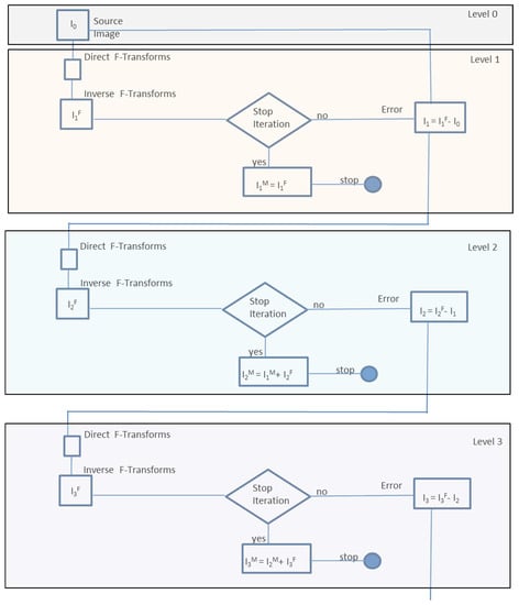
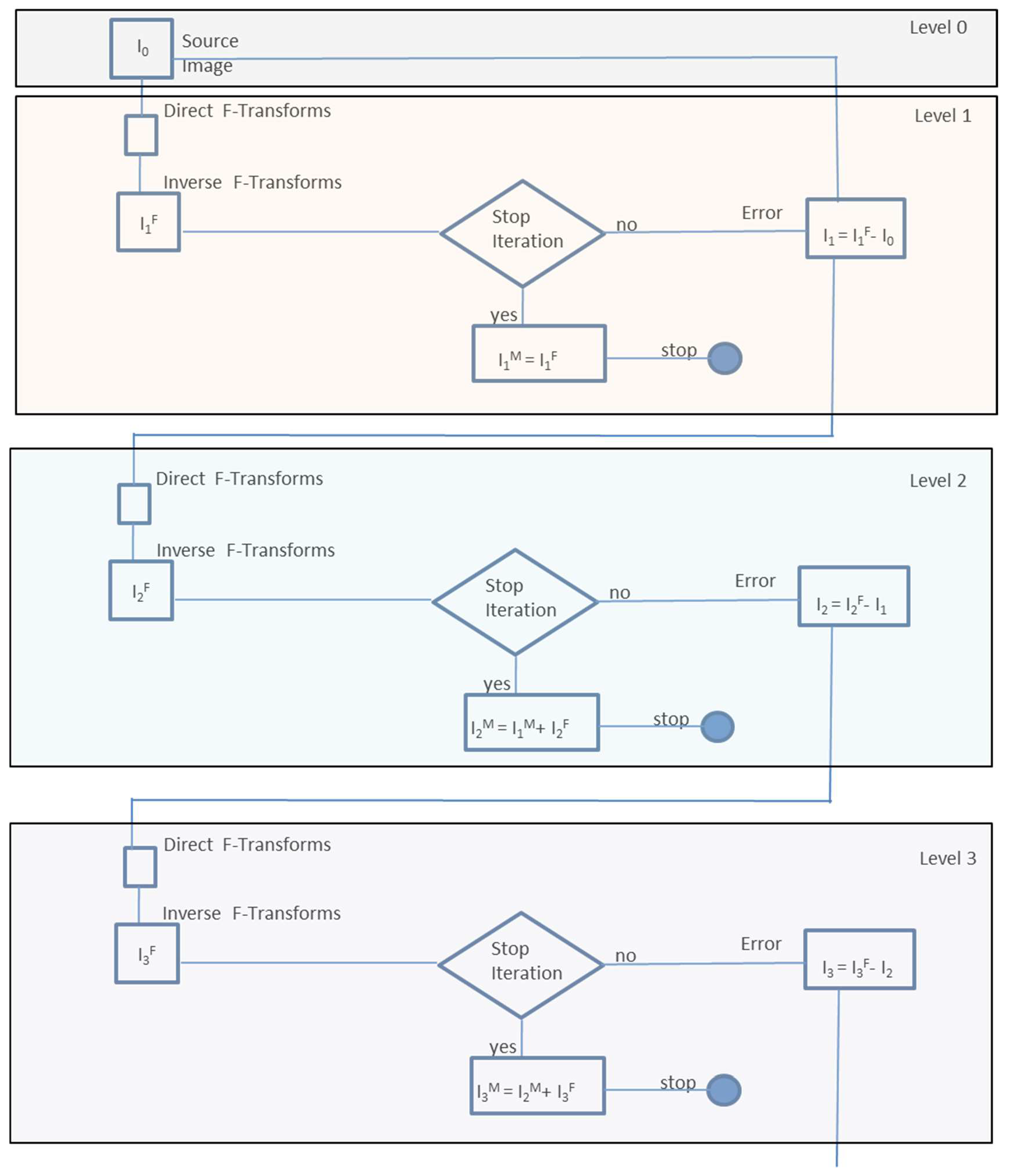
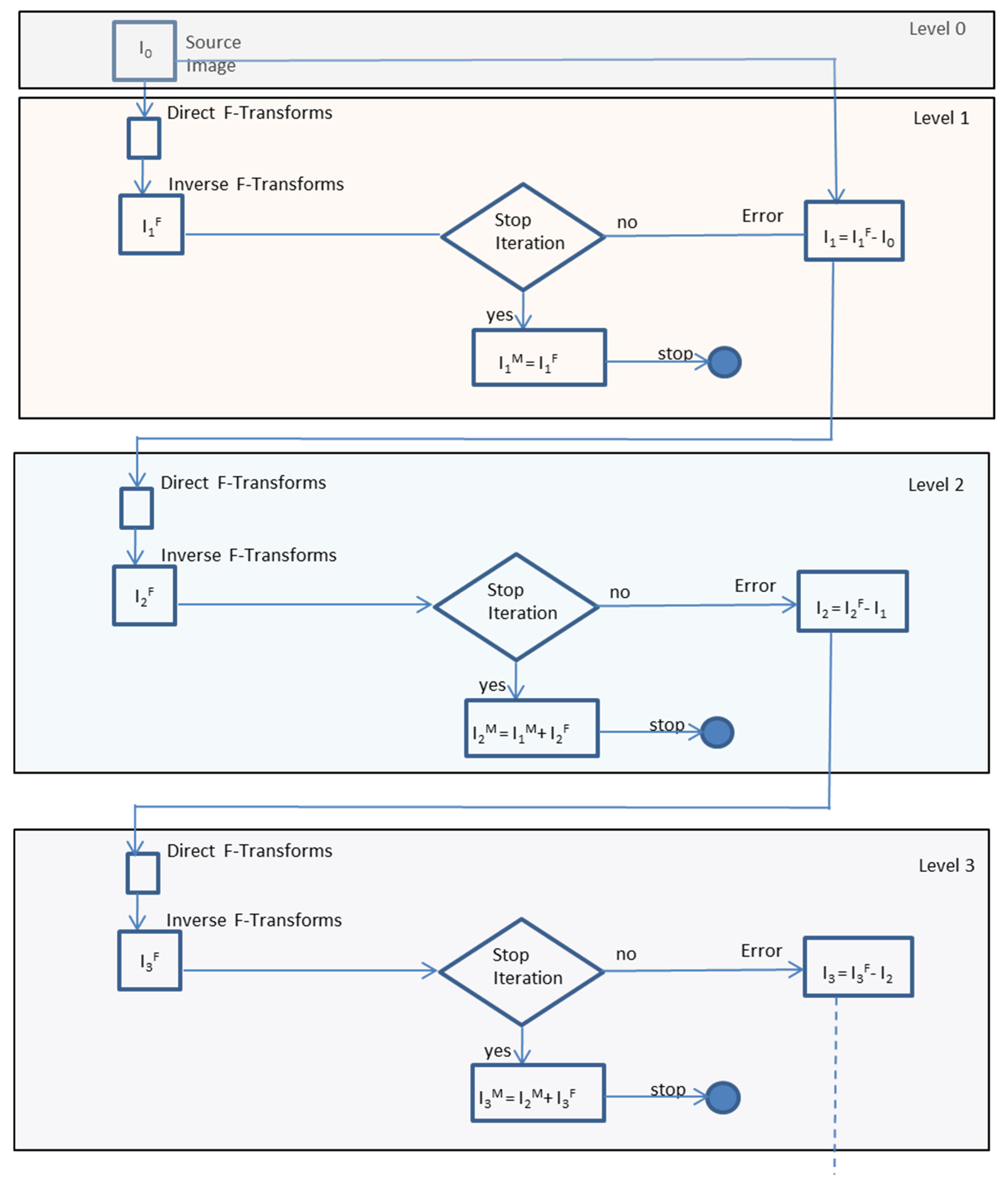
In the MF-tr algorithm, the bidimensional direct and inverse F-transforms are used to code and decode the image, respectively, at any level. The reconstructed image is given by the sum of the decoded images obtained at any level.
The image is compressed with a specified compression ratio; the input image at level zero is the source image, and the one in the succeeding level is given by the difference between the decoded (reconstructed) image and the input image in the previous level (the error).
If the quality of the reconstructed image is acceptable, then the process stops; otherwise, the error image is calculated and considered as an input image at the next level. This process is iterated until the reconstructed image is of acceptable quality. The quality of the reconstructed image is measured by computing the Peak Signal-to-Noise Ratio (PSNR) index: the quality of the reconstructed image is acceptable if the PSNR value exceeds a selected threshold.
In Figure 1, the architecture of the MF-tr method is schematized.
The main problem of this method results from a chosen compression ratio: If it is high, so that the compression is weak, the process ends quickly, leaving space for further compression. If, on the other hand, the compression ratio is small, i.e., the compression is strong, the computation time is longer because of many needed iterations.
Therefore, it is not possible to determine a priori the functional behavior of the PSNR index with respect to the compression ratio because this function depends on many characteristics of the image. As a result, it is recommended to estimate the PSNR index for images reconstructed using various compression ratios and to find the best compression ratio a posteriori as a trade-off between the compression ratio that allows us to reach an acceptable quality of the reconstructed image and the execution time.
The compression ratio is a parameter in the range [0,1] used to characterize compression by the ratio between the sizes of the compressed and source images. The aim of this research was to improve the MF-tr algorithm by proposing an approach to find the best compression ratio in the sense explained above. This compression ratio is the one which provides a reconstructed image with the quality required to pass the chosen threshold. Subsequently, the proposed MF-tr algorithm with the selected compression ratio is executed with guaranteed quality of the reconstructed image. Comparative tests with the previously proposed MF-tr algorithms were performed, and the execution times are displayed.
In Section 2, we recall the concept of bidimensional discrete direct and inverse F-transforms and describe the MF-tr method. In Section 3, we present the fast MF-tr image compression method; in Section 4, the experimental results are shown and discussed; and the conclusions are reported in Section 5.
2. Preliminaries
2.1. Discrete Dircct and Inverse F-Transforms for Coding/Decoding Images
The F-transform is a well-known technique proposed in [2] to approximate a continuous function f: X → Y in a closed interval [a,b] based on the knowledge of the value of f in a discrete set of points. The F-transform deals with a fuzzy partition of the domain X given by fuzzy sets called basic functions.
Formally, let [a,b] be a closed interval, n ≥ 2, and x1, x2, …, xn be a set of n-many points of [a,b], called nodes, such that a = x1 < x2 <…< xn = b. We say that an assigned family of fuzzy sets A1, …, An: [a,b] → [0,1], with Ai(x) a continuous function on [a,b], is a fuzzy partition of [a,b] if the following conditions hold:
- Ai(xi) = 1 for every i = 1, 2, …, n;
- Ai(x) = 0 if x is not in (xi−1, xi+1), where we assume x0 = x1 = a and xn+1 = xn = b by commodity of presentation;
- Ai(x) strictly increases on [xi−1, xi] for i = 2, …, n and strictly decreases on [xi, xi+1] for i = 1, …, n − 1;
- for every x ∈ [a,b].
The fuzzy sets {A1, …, An} are called basic functions. Moreover, we say that they form a uniform fuzzy partition if
- ▪
- n ≥ 3 and the nodes are equidistant, i.e., xi = a + h ∙ (i − 1) where h = (b − a)/(n − 1) for i = 1, 2, …, n;
- ▪
- Ai(xi − x) = Ai(xi + x) for every x ∈ [0,h] and i = 2, …, n − 1; and
- ▪
- Ai+1(x) = Ai(x − h) for every x ∈ [xi, xi+1] and i = 1,2, …, n − 1.
Let p1, …, pN be a set of points in [a,b] on which the values assumed by the function f are known. We call this set of points sufficiently dense with respect to the fuzzy partition {A1, A2, …, An} if for each basic function Ai, i = 1, …, n, there exists at least a point pj, j = 1, …, N, such that Ai(pj) > 0. In this case we can define the n-dimensional vector F = [F1, …, Fn] with components
called the discrete direct fuzzy transform of f with respect to the fuzzy partition {A1, A2, …, An}. We define the discrete inverse F-tr of the function f with respect to {A1, A2, …, An} to be the following function defined in the same points p1, …, pm of [a,b]:
where fF,n is called the discrete inverse fuzzy transform of f with respect to the fuzzy partition {A1, A2,…, An}.
Let f(x) be assigned on a set P of points p1, …, pm of [a,b]. Then, for every ε > 0, it is proved [2] that there exist an integer n(ε) and a related fuzzy partition {A1, A2, …, An(ε)} of [a,b] such that P is sufficiently dense with respect to {A1, A2, …, An(ε)} and the inequality |f(pj) − fF,n(ε)(pj)| < ε holds true for every pj ∈ [a, b], j = 1, …, m.
Now we extend these definitions to functions in two variables continuous in the rectangle [a,b] × [c,d]. Let n, m ≥ 2, and let x1, x2, …, xn ∈ [a,b] and y1, y2, …, ym ∈ [c,d] be (n + m)-many assigned points, called nodes, such that a = x1 < x2 <…< xn = b and c = y1 < …< ym = d. Furthermore, let A1, …, An: [a,b] → [0,1] be a fuzzy partition of [a,b] and B1,…,Bm: [c,d] → [0,1] be a fuzzy partition of [c,d]. Let (pj,qj) ∈ [a,b] × [c,d], where i = 1, …, N and j = 1, …, M, be a set of (N × M)-many points on which the values assumed by the function f are known. If the sets P = {p1, …, pN} and Q = {q1, …, qM} of these points are sufficiently dense, respectively, with respect to the partitions {A1, A2, …, An} and {B1, …, Bm}, then we define the bidimensional discrete direct fuzzy transform of f given by the matrix F with components
We define the bidimensional discrete inverse fuzzy transform with respect to {A1, A2, …, An} and {B1, …, Bm} to be given by
Let I be a gray image of N × M size and L gray levels. For brevity, we consider I(i,j) normalized to [0,1] (i.e., I(i,j) = P(i,j)/L, with P(i,j) the original pixel value). Let us consider the function I: (i,j) ∈ {1, …, N} × {1, …, M} → [0,1] and the fuzzy partitions A1, …, Am: [1,N]→ [0,1] of [1,N] and, B1, …, Bn: [1,M]→[0,1] of [1,M] with n < N and m < M.
We can apply the discrete direct F-transform (3) to compress the image I and the discrete inverse F-transform (4) to obtain the decoded image.
In [3,4], the matrix I was divided into submatrices IB of NB × MB size, called blocks. For any block we consider the function IB: (i, j)∈{1, …, NB} × {1, …, MB}®[0,1]), compressing the block via direct F-transform to a block of size nB × mB with nB < NB and mB < MB, obtaining
The block is reconstructed via the inverse F-transform, obtaining
The reconstructed blocks are subsequently joined to form the decompressed image. Similarly, the compressed blocks are subsequently joined to form the compressed image.
2.2. Multilevel F-Transform Image Compression
The MF-transform image compression method is an iterative method proposed in [6] where the source image is initially compressed via direct F-transform and the difference between the image reconstructed via inverse F-transform and the source image is calculated in a new image called the error. The error image is the input image of the successive phase, compressed via direct F-transform, and then the image error is calculated as well.
This process continues iteratively until the quality of the reconstituted image is higher than a fixed threshold.
Formally, let I0 be the source image. At Level 1, it is coded and decoded by using the direct and inverse F-transforms, respectively. Let be the decoded image. In [6], a set of criteria was fixed for stopping the iterations. If the iteration stop criteria are reached, the algorithm stops and the final reconstructed image is given by I1M = I1F; otherwise, the error at Level 1, I1 = − I0, is calculated, and the process is iterated at Level 2 where the image I1 is coded and decoded by using the direct and inverse F-transforms.
In general, if at Level s the iteration stop criteria are reached, the final reconstructed image obtained by applying the MF-transform method algorithm will be
Otherwise, the error image at Level s is calculated by
and the process is iterated at Level s + 1.
In [6], three stop iteration criteria based on the peak signal-to-noise ratio (PSNR) index were applied.
The PSNR index [19,20] measures the quality of the reconstructed image compared with the source image. The PSNR of the image reconstructed at Level s is obtained by calculating the mean square error MSE), given by
The PSNR index is given by the formula
where L is the number of gray levels of the image.
The PSNR index is measured in decibels; it is greater the lower the value of the MSE is; that is, the smaller the mean square error compared to the original image, the closer the PSNR approaches infinity. Then, a higher PSNR value provides a higher image quality.
The MF-tr algorithm stops if at least one of the following criteria is met:
- The PSNR of the reconstructed image at Level h is greater than a prefixed threshold PSNRth. In this case, the quality of the reconstructed image obtained is already acceptable;
- The difference between the PSNR at the sth level and the PSNR at the (s − 1)th level is less than a difference threshold DPSNRth. The algorithm stops because the contribution to the improvement of the image quality obtainable in the subsequent iterations will be of little significance;
- The process has reached the maximum number of iterations smax.
The parameters PSNRth, DPSNRth, and smax and the compression ratio ρ are set by the user.
The execution time increases with the number of levels to be reached before meeting at least one of the three criteria defined above. Therefore, the execution time depends on the choice of the compression ratio: a compression ratio that provides at Level 1 a reconstructed image of much lower quality than that required (when PSNR ≪ PSNRth) would imply a high execution time as many cycles will be required to obtain a reconstructed image of the required quality.
3. The Fast Multilevel F-Transform Image Compression Method
In order to set an optimal value for the compression ratio, we constructed a preprocessing phase in which the image is coded/decoded via F-transform by using a set of compression ratios.
Let I0 be the source image of size N × M and PSNRth be the threshold of the PSNR index. We apply the F-transform method considering the set D of compression ratios ρ1 < ρ2 < … < ρn in the range between ρmin and ρmax.
The PSNR index increases with increasing compression ratio. Thus, to find the best compression ratio, the algorithm applies the binary search strategy considering an initial compression ratio ρFirst given by the median value in the set D of compression ratios. Then, the PSNR index is calculated. If the PSNR is greater than PSNRth, then a stronger compression is performed and the previously used compression ratio is set; otherwise, a weaker compression is performed and the succeeding compression ratio is used. Now we suppose that, at a certain moment, the calculated PSNR index is greater than the threshold PSNRth, while in the previous cycle it was less than PSNRth: in this case the process stops and the compression ratio used in the previous cycle is set. Otherwise, if the PSNR index is less than PSNRth while in the previous cycle it was greater than PSNRth, the process stops and the current compression ratio is set.
Below, the Fast MF-tr Algorithm 1 is shown in pseudocode.
| Algorithm 1: Fast MF-tr | ||
| Input: | N × M source image I0 Sorted set of compression ratios {ρ1, ρ2, …, ρn} Threshold similarityPSNRth Difference threshold DPSNRth Max number of iterations smax | |
| Output: | Reconstructed image | |
| 1 | ρ:= median({ρ1, ρ2, …, ρn}) | |
| 2 | ρBest: ρ | |
| 3 | stopIteration:= FALSE | |
| 4 | PSNRold:= PSNRth | |
| 5 | WHILE (stopIteration=FALSE) | |
| 6 | Compress the source image I0 via direct F-transform | |
| 7 | Decompress the source image I0 via inverse F-transform | |
| 8 | Calculate the PSNR index (8) | |
| 9 | IF (PSNR > PSNRth) AND (PSNRold < PSNRth) THEN | |
| 10 | ρBest: = ρold | |
| 11 | stopIteration:= TRUE | |
| 12 | ELSE | |
| 13 | IF (PSNR < PSNRth) AND (PSNRold > PSNRth) THEN | |
| 14 | ρBest:= ρ | |
| 15 | stopIteration:= TRUE | |
| 16 | ELSE | |
| 17 | PSNRold:= PSNR | |
| 18 | IF (PSNR > PSNRth) THEN | |
| 19 | ρ:= ρprev | |
| 20 | ELSE | |
| 21 | ρ:= ρnext | |
| 22 | END IF | |
| 23 | ENDIF | |
| 24 | END IF | |
| 25 | END WHILE | |
| 26 | CALL MF-tr(I0, PSNRth, PSNRth, DPSNRth, smax) | |
| 27 | RETURN reconstructed image | |
Then, the F-tr algorithm is applied using the optimal compression ratio detected. This approach allows us to decrease the processing time and to reach the minimum number of iterations that will guarantee the selected quality of the reconstruction.
4. Test Results
We tested our method on a set images of sizes 256 × 256 and 512 × 512 from the Southern California Signal and Image Processing Institute (USC-SIPI) Image Database (http://sipi.usc.edu/database/) using an Intel Core i7-59360X processor with a clock frequency of 3 GHz.
In all our experiments, we considered the set of compression ratios ρ = {6.1 × 10⁻⁵, 2.44 × 10⁻⁴, 9.77 × 10⁻⁴, 3.9 × 10⁻³, 3.09 × 10⁻³, 6.94 × 10⁻³, 4.00 × 10⁻², 1.56 × 10⁻², 2.78 × 10⁻², 6.25 × 10⁻², 0.11, 0.25, 1}. The median value in this set is ρ = 4.00 × 10⁻². This was the initial compression ratio used for executing the best compression ratio search. The highest compression ratio in the set is ρ = 1, corresponding to a null compression.
We set the PSNRth threshold as the value of the PSNR index for which the trend of the PSNR index varying with the compression ratio showed an approximate plateau for gradually weaker compressions.
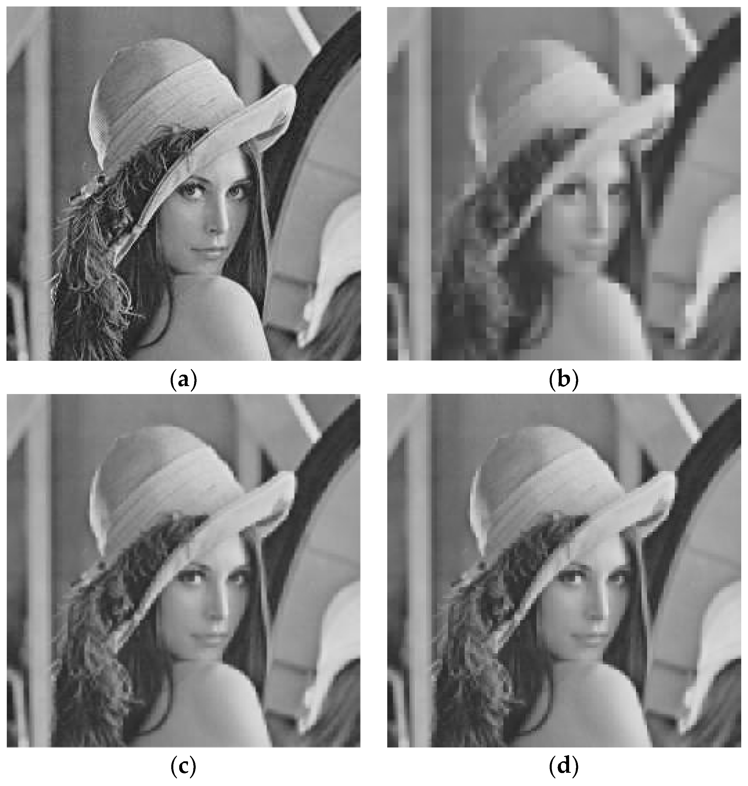
Here, we present the results obtained with the 256 × 256 image Lena, shown in Figure 3a. We set the threshold PSNRth to 28.
Initially we used the median compression ratio ρ = 4.00 × 10⁻², obtaining a PSNR value of 23.87. In Figure 3b, we show the decompressed image obtained. The best compression ratio was ρBest = 0.11. In Figure 3c, we show the corresponding decompressed (reconstructed) image; the PSNR was 27.68. Using a smaller compression ratio than ρ = 0.11, we obtained PSNR = 28.41, which is greater than the threshold value.
In Figure 3d, we show the final reconstructed image obtained by applying the Fast MF-tr algorithm. It was computed at Level 2, and the final PSNR was 28.29. Applying the MF-tr algorithm by considering an initial compression ratio of ρ = 4.00 × 10⁻², the reconstructed image was obtained at Level 6.
Table 1 shows the comparison results obtained by using the MF-tr and the proposed algorithm. In addition to the PSNR, the calculated value of the structural similarity index (SSIM) for measuring the quality of the reconstructed image is also shown. These results highlight that the CPU time needed for coding the image obtained by using the Fast F-tr algorithm was about half that required by running the MF-tr algorithm. The reconstructed image has the same quality as the image reconstructed by the MF-tr algorithm method, as measured using the PSNR and SSIM indices.
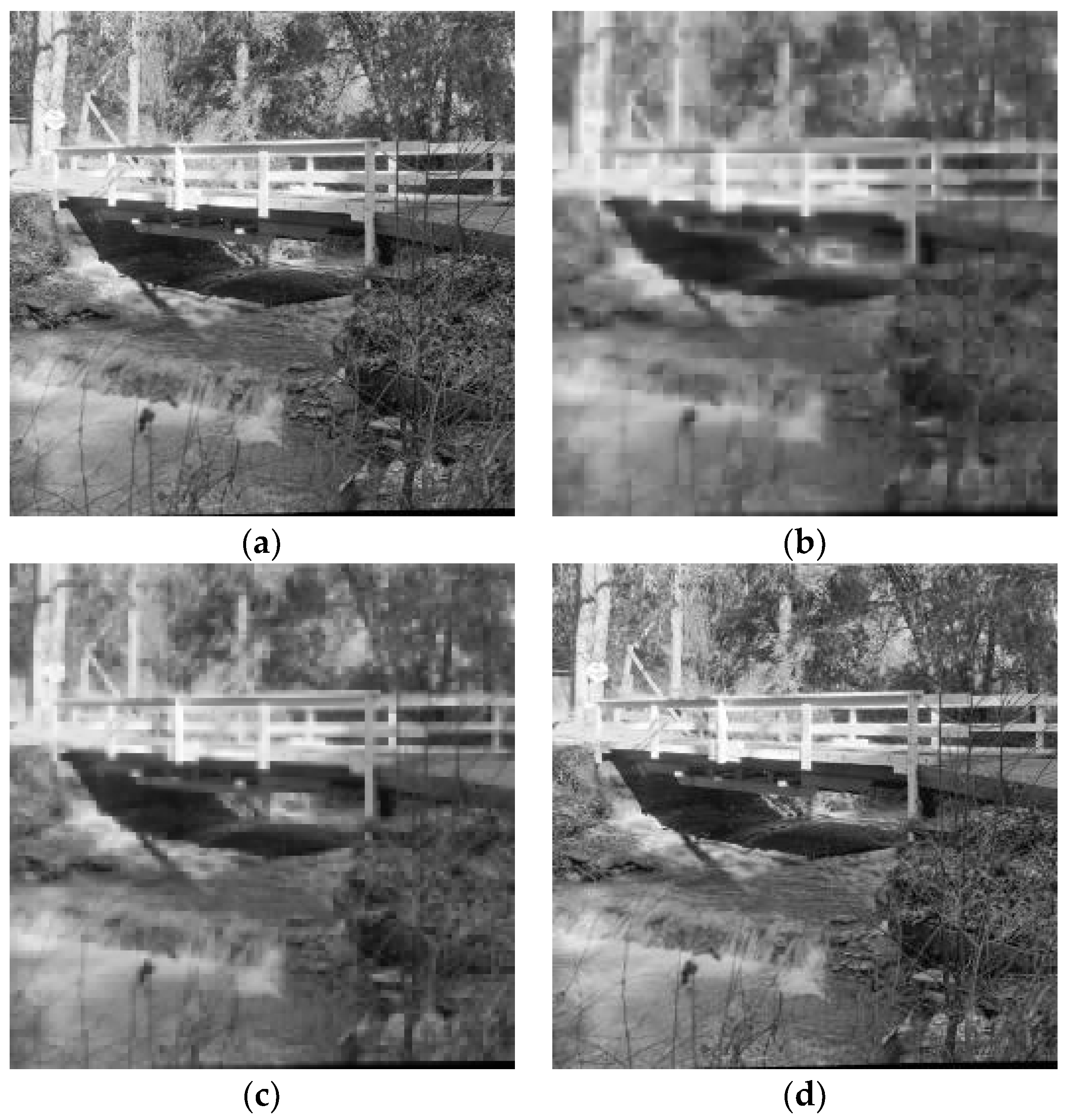
Below we show the results obtained using the source 512 × 512 gray image Bridge (Figure 4a). We set the threshold PSNRth to 25. By using the median compression ratio ρ = 4.00 × 10⁻², we obtained a PSNR value of 20.79 (Figure 4b); the best compression ratio was ρBest = 6.25 × 10⁻², and the corresponding PSNR was 24.38 (Figure 4c). The final image was reconstructed at the second level, obtaining PSNR = 25.16 (Figure 4d).
Table 2 shows the comparison results with respect to the MF-tr algorithm. Using the MF-transform algorithm, a reconstructed image with PSNR = 25.15 and SSIM = 0.91 was obtained at the fifth level, with a CPU time of 74.65 s. Using the Fast MF-tr algorithm, the reconstructed image (PSNR = 25.16, SSIM = 0.92) was obtained at the second level, and the CPU time (33.28 s) was, also in this case, about half that obtained via the MF-tr algorithm.
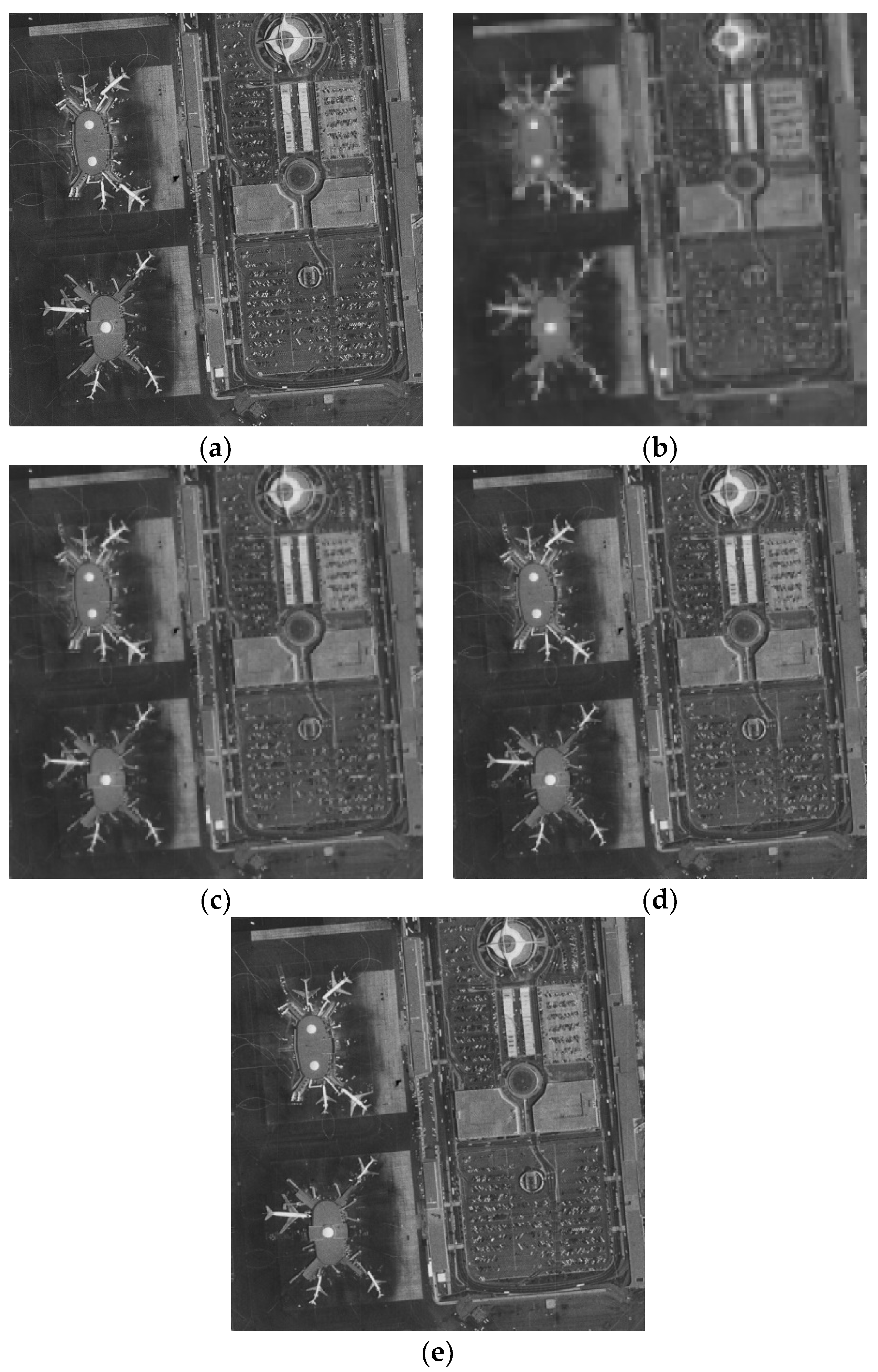
Finally, we show the results obtained with the source 1024 × 1024 gray image Airport (Figure 5a). The threshold PSNRth was set to 28. By using the median compression ratio ρ = 4.00 × 10⁻², we obtained a PSNR value of 22.05 (Figure 4b); the best compression ratio was ρBest = 0.11 and the corresponding PSNR was 27.87 (Figure 5d). The final image was reconstructed at the third level, obtaining PSNR = 28.10 (Figure 5e).
Table 3 shows the comparison results with respect to the MF-tr algorithm. Using the MF-transform algorithm, a reconstructed image with PSNR = 28.12 and SSM = 0.94 was obtained at the fifth level, with a CPU time of 151.18 s. Using the Fast MF-tr algorithm, the reconstructed image (PSNR = 28.10, SSIM = 0.94) was obtained at the third level; the CPU time was 54.86—almost one-third of that obtained via the MF-tr algorithm.
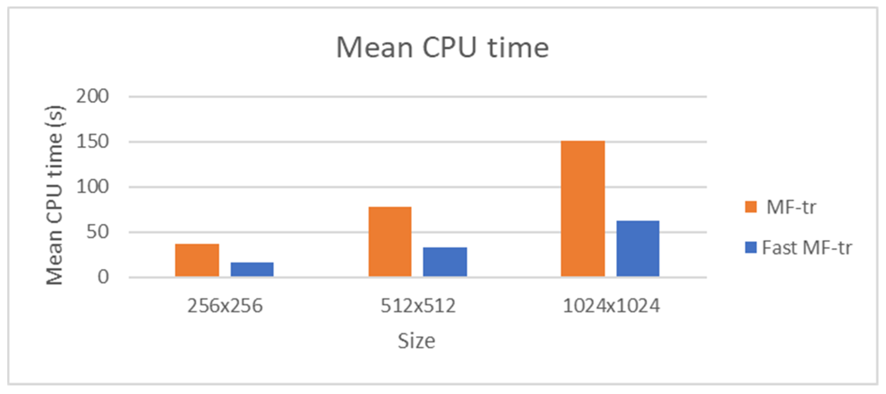
In the histogram in Figure 6, we show the respective mean CPU times obtained by applying the two algorithms on images with sizes 256 × 256, 512 × 512, and 1024 × 1024.
The last column in Table 4 shows the ratio between the mean CPU time obtained by using the Fast MF-tr algorithm and the mean CPU time obtained by using the MF-tr algorithm. This ratio is always less than 0.5 and decreases with increasing image size.
These results show that the execution times measured using the Fast MF-tr algorithm were always less than half the execution times measured using the MF-tr algorithm.
5. Conclusions
We proposed a fast variant of the MF-tr image compression algorithm, in which the best compression ratio is found and then applied in order to obtain a reconstructed image with quality greater than a preselected threshold. We compared our algorithm with the F-tr algorithm, applying both to 256 × 256, 512 × 512, and 1024 × 124 images from the USC-SIPI Image Database.
The comparison results show that the execution time of the newly proposed Fast F-tr algorithm is less than one-half of the execution time of the MF-tr algorithm.
In the future, we intend to do further tests applying the Fast MF-tr algorithm to large images, such as high-resolution satellite or medical images, in order to develop an optimal method of compressing large images that is capable of preserving image quality and, at the same time, of guaranteeing reasonable execution time.
Author Contributions
The contributions of the three authors Ferdinando Di Martino (FD), Irina Perfilieva (IP), and Salvatore Sessa (SS) are summarized below: conceptualization, F.D., I.P. and S.S..; methodology, F.D., I.P. and S.S.; software, F.D., I.P. and S.S.; validation, F.D., I.P. and S.S.; formal analysis, F.D., I.P. and S.S.; investigation, F.D., I.P. and S.S.; resources, X.X.; data curation, F.D., I.P. and S.S.; writing—original draft preparation, F.D., I.P. and S.S.; writing—review and editing, F.D., I.P. and S.S.; visualization, F.D., I.P. and S.S.; supervision, F.D., I.P. and S.S.
Funding
This research received no external funding.
Acknowledgments
The work of Ferdinando Di Martino and Salvatore Sessa was supported by the Centro Interdipartimentale Alberto CalzaBini, University of Naples Federico II, Via Toledo, 402 - 80132 - Naples (Italy). The work of Irina Perfilieva was supported by the Czech Ministry of Education, Youth and Sports, project OP VVV (AI-Met4AI): No. CZ.02.1.01/0.0/0.0/17-049/0008414.
Conflicts of Interest
The authors declare no conflict of interest.
References
- Perfilieva, I. Fuzzy transforms. Fuzzy Sets Syst. 2006, 157, 993–1023. [Google Scholar] [CrossRef]
- Di Martino, F.; Sessa, S. Compression and decompression of images with discrete fuzzy transforms. Inf. Sci. 2007, 17, 2349–2362. [Google Scholar] [CrossRef]
- Di Martino, F.; Loia, V.; Perfilieva, I.; Sessa, S. An image coding/decoding method based on direct and inverse fuzzy transforms. Int. J. Approx. Reason. 2008, 48, 110–131. [Google Scholar] [CrossRef] [Green Version]
- Di Martino, F.; Loia, V.; Sessa, S. Fuzzy transforms for compression and decompression of colour videos. Inf. Sci. 2010, 180, 3914–3931. [Google Scholar] [CrossRef]
- Perfilieva, I.; De Baets, B. Fuzzy transforms of monotone functions with application to image compression. Inf. Sci. 2010, 180, 3304–3315. [Google Scholar] [CrossRef]
- Di Martino, F.; Sessa, S. A Multi-Level Image Compression Method Based on Fuzzy Transforms. J. Ambient Intell. Humaniz. Comput. 2019, 10, 2745–2756. [Google Scholar] [CrossRef]
- Toet, A. A morphological pyramidal image decomposition. Pattern Recognit. Lett. 1989, 9, 255–261. [Google Scholar] [CrossRef]
- Paris, S.; Hasinoff, S.V.; Kautz, J. Local Laplacian filters: Edge-aware image processing with a Laplacian pyramid. Commun. ACM 2015, 58, 81–91. [Google Scholar] [CrossRef]
- Boiangiu, C.A.; Cotofana, M.V.; Naiman, A.; Lambru, C. A generalized Laplacian Pyramid aimed at image compression. J. Inf. Syst. Oper. Manag. 2016, 10, 327–335. [Google Scholar]
- Ispas, C.; Boiangiu, C.A. An image compression scheme based on Laplacian Pyramid. J. Inf. Syst. Oper. Manag. 2017, 11, 350–358. [Google Scholar]
- Walker, J.S.; Nguyen, T.Q. Wavelet-Based Image Compression (Chapter 6). In The Transform and Data Compression Handbook; Rao, K.R., Yip, P.C., Eds.; CRC Press LLC: Boca Raton, FL, USA, 2001. [Google Scholar]
- Song, M.-S. Wavelet Image Compression. Contemp. Math. 2006, 414, 41–73. [Google Scholar]
- Khan, U.R.; Ahmed, S.; Nazeer, T. Wavelet Based Image Compression Techniques: Comparative Analysis and Performance Evaluation. Int. J. Emerg. Technol. Eng. Res. 2017, 5, 9–13. [Google Scholar]
- Karthikeyan, C.; Palanisamy, C. An Efficient Image Compression Method by Using Optimized Discrete Wavelet Transform and Huffman Encoder. J. Comput. Theor. Nanosci. 2018, 15, 289–298. [Google Scholar] [CrossRef]
- Perfilieva, I. Fuzzy transform in image compression and fusion. Acta Math. Univ. Ostrav. 2007, 15, 27–37. [Google Scholar]
- Perfilieva, I.; Dankova, M. Image fusion on the basis of fuzzy transforms. In Proceedings of the 8th International FLINS Conference on Computational Intelligence in Decision and Control, Madrid, Spain, 21–24 September 2008; pp. 471–476. [Google Scholar]
- Manchanda, M.; Sharma, R. A novel method of multimodal medical image fusion using fuzzy transform. J. Vis. Commun. Image Represent. 2016, 40, 197–217. [Google Scholar] [CrossRef]
- Di Martino, F.; Sessa, S. Complete image fusion method based on fuzzy transforms. Soft Comput. 2019, 23, 2113–2123. [Google Scholar] [CrossRef]
- Huynh-Thu, Q.; Ghanbari, M. Scope of validity of PSNR in image/video quality assessment. Electron. Lett. 2008, 44, 800–801. [Google Scholar] [CrossRef]
- Huynh-Thu, Q.; Ghanbari, M. The accuracy of PSNR in predicting video quality for different video scenes and frame rates. Telecommun. Syst. 2012, 49, 35–48. [Google Scholar] [CrossRef]
Figure 1.
Multilevel structure in the multilevel F-transform (MF-tr) algorithm.

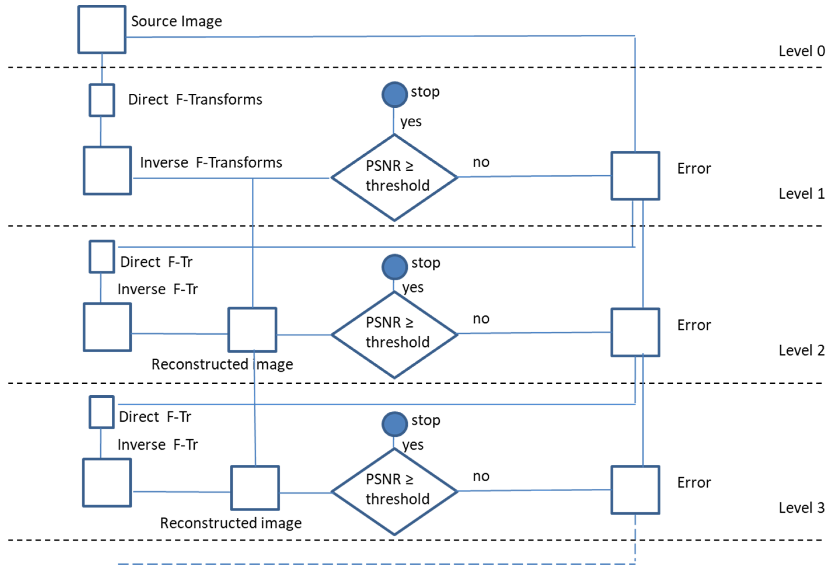
Figure 2.
The multilevel F-transform image reconstruction process.

Figure 3.
(a) Source image: Lena. (b) Decompressed image at Level 1 (ρ = 4.00 × 10⁻²); (c) Decompressed image at Level 2 (ρ = 0.11). (d) Final reconstructed image.
Figure 3.
(a) Source image: Lena. (b) Decompressed image at Level 1 (ρ = 4.00 × 10⁻²); (c) Decompressed image at Level 2 (ρ = 0.11). (d) Final reconstructed image.

Figure 4.
(a) Source image: Bridge. (b) Decompressed image at Level 1 (ρ = 4.00 × 10⁻²). (c) Decompressed image at Level 2 (ρ = 6.25 × 10⁻²). (d) Final reconstructed image.
Figure 4.
(a) Source image: Bridge. (b) Decompressed image at Level 1 (ρ = 4.00 × 10⁻²). (c) Decompressed image at Level 2 (ρ = 6.25 × 10⁻²). (d) Final reconstructed image.

Figure 5.
(a) Source image: Airport. (b) Decompressed image at Level 1 (ρ = 4.00 × 10⁻²). (c) Decomposed image at Level 2 (ρ = 6.25 × 10⁻²). (d) Decomposed image at Level 3 (ρ = 0.11). (e) Final reconstructed image.
Figure 5.
(a) Source image: Airport. (b) Decompressed image at Level 1 (ρ = 4.00 × 10⁻²). (c) Decomposed image at Level 2 (ρ = 6.25 × 10⁻²). (d) Decomposed image at Level 3 (ρ = 0.11). (e) Final reconstructed image.

Figure 6.
Histogram of the mean CPU times for images with different size.


Table 1.
PSNR, structural similarity index (SSIM), and CPU times obtained for the 256 × 256 gray image Lena.
Table 1.
PSNR, structural similarity index (SSIM), and CPU times obtained for the 256 × 256 gray image Lena.
| Algorithm | Levels | PSNR | SSIM | CPU Time (s) |
|---|---|---|---|---|
| MF-tr | 6 | 28.26 | 0.95 | 35.08 |
| Fast MF-tr | 2 | 28.29 | 0.96 | 17.57 |
Table 2.
PSNR, SSIM, and CPU times obtained for the 512 × 512 gray image Bridge.
| Algorithm | Levels | PSNR | SSIM | CPU Time (s) |
|---|---|---|---|---|
| MF-tr | 5 | 28.12 | 0.91 | 74.65 |
| Fast MF-tr | 2 | 28.10 | 0.92 | 33.28 |
Table 3.
PSNR, SSIM, and CPU times obtained for the 512 × 512 gray image Airport.
| Algorithm | Levels | PSNR | SSIM | CPU Time (s) |
|---|---|---|---|---|
| MF-tr | 7 | 25.15 | 0.94 | 148.25 |
| Fast MF-tr | 3 | 25.16 | 0.94 | 59.86 |
Table 4.
Mean CPU times obtained for different image sizes.
| Size | Mean CPU Time (s) | ||
|---|---|---|---|
| MF-tr | Fast MF-tr | CPU Time Ratio | |
| 256 × 256 | 37.11 | 17.09 | 0.46 |
| 512 × 512 | 78.29 | 33.35 | 0.43 |
| 1024 × 1024 | 151.13 | 62.54 | 0.41 |
© 2019 by the authors. Licensee MDPI, Basel, Switzerland. This article is an open access article distributed under the terms and conditions of the Creative Commons Attribution (CC BY) license (http://creativecommons.org/licenses/by/4.0/).
Share and Cite
MDPI and ACS Style
Di Martino, F.; Perfilieva, I.; Sessa, S. A Fast Multilevel Fuzzy Transform Image Compression Method. Axioms 2019, 8, 135. https://0-doi-org.brum.beds.ac.uk/10.3390/axioms8040135
AMA Style
Di Martino F, Perfilieva I, Sessa S. A Fast Multilevel Fuzzy Transform Image Compression Method. Axioms. 2019; 8(4):135. https://0-doi-org.brum.beds.ac.uk/10.3390/axioms8040135
Chicago/Turabian StyleDi Martino, Ferdinando, Irina Perfilieva, and Salvatore Sessa. 2019. "A Fast Multilevel Fuzzy Transform Image Compression Method" Axioms 8, no. 4: 135. https://0-doi-org.brum.beds.ac.uk/10.3390/axioms8040135
Note that from the first issue of 2016, this journal uses article numbers instead of page numbers. See further details here.