Article

Determination of the Distribution of Relaxation Times by Means of Pulse Evaluation for Offline and Online Diagnosis of Lithium-Ion Batteries

Electrical Energy Storage Technology, Departement of Energy and Automation Technology, Faculty IV, Secr. EMH 2, Technische Universität Berlin, Einsteinufer 11, D-10587 Berlin, Germany
*
Author to whom correspondence should be addressed.
Submission received: 26 February 2021 / Revised: 19 March 2021 / Accepted: 2 April 2021 / Published: 1 June 2021
(This article belongs to the Special Issue Battery Systems and Energy Storage beyond 2020)

Abstract

:
The distribution of relaxation times (DRT) analysis of impedance spectra is a proven method to determine the number of occurring polarization processes in lithium-ion batteries (LIBs), their polarization contributions and characteristic time constants. Direct measurement of a spectrum by means of electrochemical impedance spectroscopy (EIS), however, suffers from a high expenditure of time for low-frequency impedances and a lack of general availability in most online applications. In this study, a method is presented to derive the DRT by evaluating the relaxation voltage after a current pulse. The method was experimentally validated using both EIS and the proposed pulse evaluation to determine the DRT of automotive pouch-cells and an aging study was carried out. The DRT derived from time domain data provided improved resolution of processes with large time constants and therefore enabled changes in low-frequency impedance and the correlated degradation mechanisms to be identified. One of the polarization contributions identified could be determined as an indicator for the potential risk of plating. The novel, general approach for batteries was tested with a sampling rate of 10 Hz and only requires relaxation periods. Therefore, the method is applicable in battery management systems and contributes to improving the reliability and safety of LIBs.

1. Introduction

The use of energy storage systems is essential for the transition to renewable energies. Due to the unsteady energy supply from renewable energies such as wind power and photovoltaics, energy storage devices are required to compensate for fluctuations in output and to reliably provide energy at all times. For the electrification of the transport sector, energy storage systems are required in order to move vehicles independently of an external energy supply and without burning fossil fuels. In battery electric vehicles in particular, LIBs are by far the most frequently used battery technology due to their high energy and power density.
Large batteries are required in electric vehicles (EVs) and stationary energy storage devices, which are therefore the main cost factor in these applications. Accordingly, the requirements for the service life of the LIBs are high and a high degree of reliability is a prerequisite.
Therefore, non-invasive investigation methods are used to achieve a comprehensive understanding of the underlying degradation mechanisms of LIBs to enable system optimizations with regard to the service life. In addition, the non-invasive methods are required for the online diagnosis of LIBs and to identify potential risks during operation in order to ensure safe operation.
In current studies, the continous determination of the changes in kinetic parameters of LIBs made it possible to draw conclusions about progressive aging and degradation mechanisms [1,2,3,4,5]. Compared to recording of the open-circuit-voltage (OCV) or to directly determining the capacity, measuring the dynamic behavior of LIBs is usually less time-consuming [1].
EIS as a non-invasive technique is widely used for aging studies in order to measure the impedance directly and thus to determine the kinetic parameters of the LIBs [6,7,8,9]. Aging processes such as lithium plating [3] and the formation of the solid electrolyte interface (SEI) [4] could be investigated using EIS.
The derivation of the DRT on the basis of the EIS measurement data as well as the further DRT analysis is a common method for the investigation of LIBs and other batteries. In [10,11,12,13,14,15] methods are investigated and described to obtain the DRT from impedance data. In several publications, the number of dominant electrochemical processes of LIB as well as their time constants and polarization contributions could be quantified by analyzing the DRT of the measured spectra [14,15,16,17]. Changes in the time constants and polarization contributions during the aging of the LIBs under investigation can also be determined using the DRT, as recently shown by Sabet et al. [5].
The main disadvantage of EIS is the long measurement time, especially for low frequencies. The measurement time ranges from several hours for frequencies in the millihertz range to several days for frequencies in the microhertz range. Therefore the bandwidth and resolution of the impedance measurement data available for the DRT is limited [15]. Additionally, only small signal amplitudes are permitted to ensure that the steady state condition is not violated during the EIS. The long measuring times and low signal amplitudes cannot be implemented under operating conditions and with commercially available measuring electronics [18], which is why DRT analyzes have so far been limited to laboratory tests. But even under laboratory conditions, when measuring lower frequencies, maintaining the steady state and current drift are becoming increasingly critical [19].
Due to the general availability in online applications, the characterization of cell impedance based on pulse data is of great interest and the subject of some current studies (e.g., [20,21]). The time domain data of current and voltage curves can be evaluated in the event of pulse excitations in order to determine the impedance of the LIB and other battery types. The calculation on the basis of time domain data is generally faster than the direct measurement of the impedance, since several frequencies are excited simultaneously with excitations in the time domain [19]. Thus, on the basis of time domain data, a higher frequency resolution and wider bandwidth of the impedance measurements can be achieved, which is of particular interest with regard to the DRT.
An overview of the options for calculating the impedance using time domain data is given in [22]. In [19,23], the time domain data resulting from pulse measurements were brought into the frequency domain using a fast Fourier transform (FFT) in order to calculate the low frequency impedance. However, the excitation of a pulse is non-periodic. A window function must therefore be used for the transformations, which in turn generates an offset of the signal [18]. To avoid additional sources of error, as an alternative to the FFT or Laplace transformation, a pre-selected equivalent circuit model (ECM) can be parameterized using the time domain data [19]. The impedance is obtained by transforming the ECM into the frequency domain. The ECM is chosen in a manner that the impedance behavior of the battery can be reproduced. Therefore, the model must be selected individually for each battery type, cell chemistry and the electrochemical processes to be expected [24]. In addition, the impedance of the batteries can change significantly with aging, state of charge (SOC) as well as temperature and thus also the dynamic behavior in the time domain. For this reason, prior knowledge of the electrochemical processes involved and of the aging behavior and further dependencies is required in order to select a suitable model.
The DRT can be derived from the calculated impedance. If the selected ECM consists only of RC elements (parallel connection of resistance and capacitor) and an internal resistance (Thévenin model), the DRT is given directly by the model in the time domain and a transformation to frequency domain is not necessary. Analytical methods have already been proposed for the online parameterization of a Thévenin model [20,25] but the number of RC elements is limited and too small to be able to derive a DRT with adequate resolution. The sufficient number of RC elements can be characterized by iterative numerical optimization methods such as genetic algorithms and method of least squares. Compared to the analytical methods, however, the computationally intensive iterative calculations are disadvantageous for online applications [25] and the number of RC elements is limited again due to the computing power available [26]. The initial values to be determined also require prior knowledge of the electrochemical processes and their approximate time constants and polarization contributions.
In summary, it can be stated that based on the analysis of the DRT, aging mechanisms have already been examined in numerous investigations. The DRT is determined according to the state of the art on the basis of the impedance. The direct measurement of the impedance by means of EIS cannot be implemented in current online applications without adaptations and at low frequencies, even under laboratory conditions, it is time-consuming and subject to inaccuracies. The indirect determination of the impedance based on the evaluation of time domain data leads to additional inaccuracies or requires an individual definition of a model for different cell chemistries and types. A direct derivation of the DRT based on time domain data, which can also be used online, would therefore be desirable.
In this study a method is proposed and described to derive the DRT directly from the measured voltage course during cell relaxation. The method is validated experimentally by comparing the results with a DRT obtained from EIS measurements. In an aging study, the introduced method and a subsequent DRT analysis are used to identify the time constants and polarization contributions of the electrochemical processes of LIBs. The method is shown to be sufficiently sensitive to quantify the changes in these parameters during aging without the need for EIS equipment or other devices not available in online applications. The study demonstrates that the DRT derived from time domain data offers significantly more insights into processes with large time constants respectively low-frequency impedance with less expenditure of time than a DRT derived from EIS measurements. In addition, a correlation between a polarization contribution of one of the processes with a large time constant and a degradation mechanism could be established. Thus, the proposed method offers a time-effective estimate of the kinetic parameters of a LIB, provides insights into battery degradation and is offline and online applicable.

2. Methods

Multiple electrochemical processes with a wide range of time constants occur in LIBs. In addition to the the charge transfer processes of the individual electrodes, diffusion processes such as solid state diffusion and diffusion of lithium ions through the surface films of the electrodes also influence the dynamic characteristics of LIBs [9]. Some processes have similar time constants and are therefore not easy to distiguish from each other only considering the spectra obtained by EIS. In Figure 1a, a spectrum of the cells examined in this research is shown.
The diffusion branch at low frequencies can be clearly assigned to the solid state diffusion as the time constant of these processes is usually a few decades larger compared to other dynamic processes [9]. The semicircle in the spectra is caused by charge transfer processes and the diffusion trough the SEI [27]. Since the time constants are of a comparable order of magnitude, these processes show overlapping effects in the impedance spectra and only a single semicircle is visible. Changes of the polarization contribution and time constants of the various processes during aging can therefore not be reliably separated and assigned to the specific processes. An approach to identify the single processes and their parameters is an analysis of the DRT [14].

2.1. DRT of Frequency Domain Data

Since the DRT analysis of frequency domain data is well-established and the focus of this study is the DRT of time domain data the method is only briefly described. We refer to [15] for a more detailed explanation of the procedure used.
In order to calculate the DRT using frequency domain data, the resistive–capacitive part of the given spectra is reconstructed with a series of m RC-elements, a parallel circuit of an ohmic resistor and a capacitor.
Z R C , s i n g l e = R 1 + j ω R C = R 1 + j ω τ
Z R C , s e r i e s = k = 1 m h ( τ k ) 1 + j ω τ k
where h ( τ k ) are the RC-elements unknown polarization contributions. By pre-defining the time constants τ = R · C , the equation of the RC elements and thus the optimization problem become linear. In view of the nature of electrochemical processes, an equidistant distribution on a logarithmic scale is assumed for the time constants. The range of time constants is expanded by two decades and the number of RC-elements per decade is increased by a factor of three compared to the measured frequencies in order to enhance the accuracy and to obtain an adequate resolution of the DRT (see e.g., [15]).
Since the number of RC-elements per decade is higher than the resolution of the impedance data, the optimization problem becomes ill-posed. Therefore, a regularization technique which was introduced by Tikhonov [28] is used to enable an analytical solution. The Tikhonov regularization for determining the DRT has already been shown in some publications [11,13,14,15]. The regularization parameter was elected according to [15]. The value is kept constant for the evaluation of all spectra, since the results of the DRT analysis are sensitive to the parameter. Thus, the DRTs of the different spectra are comparable and changes in the dispersion due to the aging process which can be tracked.
The parts of the measured spectra with positive imaginary values cannot be modelled by a series of RC-elements and have to be discarded. Additionally, the internal resistance R i is subtracted from impedance values of the measured spectra prior to the fitting procedure. It is assumed that R i is equal to the zero crossing of the imaginary axis [9]. After preprocessing of the measurement data, the spectra mainly consist of resistive–capacitive contributions, which can be modelled by RC-elements.
The optimization problem is solved with a non-negative least squares fit because only positive resistances are physically meaningful. Figure 1b depicts the DRT of the spectrum shown in Figure 1a. The position of the peaks indicate the time constants of the processes involved and the area under the peaks correlates to the polarization contribution of the process [14,15,16]. In contrast to the Nyquist diagram, which shows only a single semicircle at moderate frequencies, various processes with different polarization contributions and time constants are visible in the same frequency range.

2.2. DRT of Time Domain Data

2.2.1. General Approach

Figure 2a shows the simulation of the cell voltage of an LIB during a charge pulse with constant current and the subsequent relaxation period. The impedance of the battery was modelled by three RC-elements and internal resistance. White noise was added to the voltage signal to take measurement inaccuracies of real-world applications into account.
For the proposed method of an DRT analysis of time domain data, the voltage relaxation is evaluated. Similar to the DRT analysis of frequency domain data, an attempt is made to reconstruct the voltage behaviour with a series of RC-elements. The voltage course of a single RC-element during a relaxation period can be described as follows:
u R C ( t ) = U 0 · e t τ R C
where τ R C = R · C , the characteristic time constant of a RC-element. The voltage of the RC-element at the beginning of the relaxation period U 0 at t = 0   s can be calculated if the duration t c p and current I c p of the previous pulse are known:
U 0 = R · I c p 1 e t c p τ R C
Equation (4) is only valid if the cell has been sufficiently relaxed before the current pulse and any overvoltages can be neglected. Assuming a finite number m of RC-elements, the overall voltage response can be computed numerically:
U R C , s e r i e s ( t ) = k = 1 m R k · I c p 1 e t c p τ k · e t τ k
By defining fixed time constants τ k , the optimization problem becomes linear. The values of the resistances R k must be set in such a way that the error between the voltage prediction by the series of RC-elements and the measured voltage data (or in this case the simulated voltage data) is minimized. Using the sum of squared errors as a cost function leads to the following optimization problem m i n { J } :
J = A · R v e c U v e c 2
where the vector R v e c corresponds to the unknown polarization contributions of the RC-elements
R v e c = R 1 R k R m T
and U v e c is the vector of the measured (or simulated) voltage course:
U v e c = U 1 U n
The number n corresponds to the number of measurement points. The measurement data should be preprocessed in advance. In Section 2.2.3, a detailed description of the process is given. The dimension of the matrix A is n · m and the matrix is calculated for the different predefined constants and the time after the end of the pulse t which corresponds to the respective voltage measurement in U v e c .
A = I c p · 1 e t c p τ 1 · e t 1 τ 1 1 e t c p τ m · e t 1 τ m 1 e t c p τ 1 · e t n τ 1 1 e t c p τ m · e t n τ m

2.2.2. Predefinition of Time Constants τ

A logarithmically uniform distribution is defined for the time constants τ 1 τ m . The minimum and the maximum time constants τ m i n and τ m a x are determined based on the maximum sampling rate f s , m a x = 1 Δ t m i n and the duration of the relaxation process t m a x . The Shannon theorem states that frequencies that are higher than half of the sampling rate cannot be evaluated without further processing of the measured signal.
f e v a l , m a x 1 2 · Δ t m i n
Taking into account the transient frequency f t = 1 2 · π · τ of a RC-element, the following relationship result for the smallest observable time constant τ e v a l , m i n [29]:
1 2 · π · τ e v a l , m i n 1 2 · Δ t m i n
τ e v a l , m i n = Δ t m i n π
The largest evaluable time constant τ e v a l , m a x is limited by the duration of the relaxation phase according to [19].
f e v a l , m i n 4 t m a x
τ e v a l , m a x = t m a x 8 π
The minimum and maximum time constants of the distribution τ m i n and τ m a x are chosen to be two decades smaller, respectively, andlarger than the evaluable time constants in order to increase the accuracy at both ends of the frequency dispersion:
τ m i n = τ e v a l , m i n 100 = τ 1
τ m a x = τ e v a l , m a x · 100 = τ m
This procedure was similarly proposed by [15] for the DRT analysis of frequency domain data. In order to obtain a smooth DRT curve within the evaluated frequency range, the number of RC elements or time constants m must be selected to be high enough. A number of one hundred τ per decade was used for the analysis of the DRT in this study.

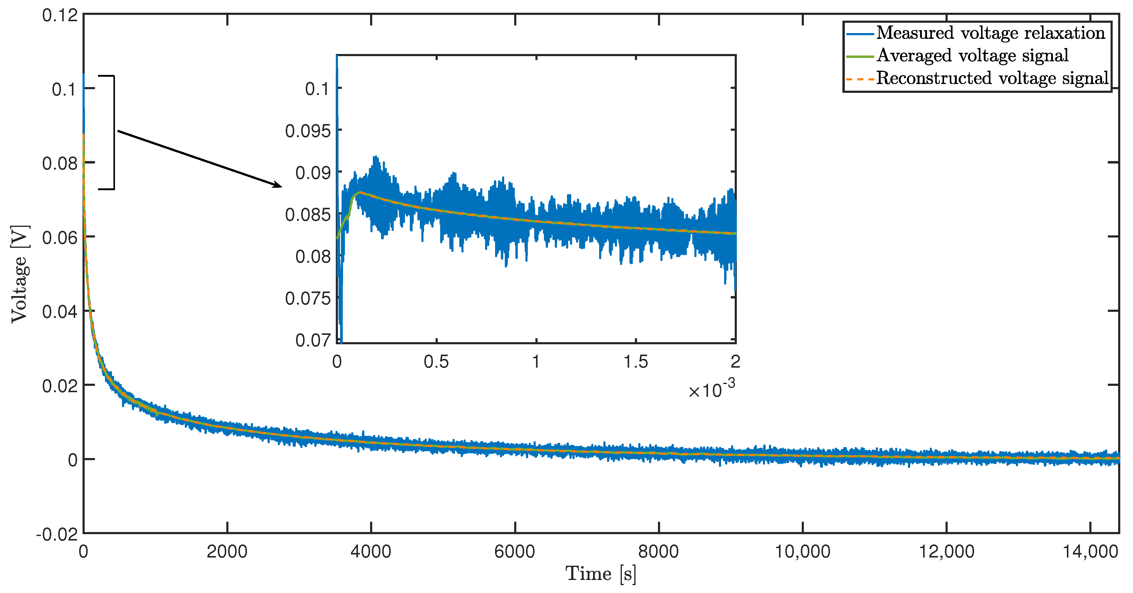
2.2.3. Pre-Processing of Measurement Data

Before calculating the DRT, the existing measurement data should be checked for usability and preprocessed. According to the Equation (12), the sampling rate must be high enough (or the timestep between two successive voltage measurements Δ t m i n small enough) to enable a meaningful evaluation of the DRT down to the time constant τ e v a l , m i n . Therefore, when selecting the the sampling rate beforehand, the minimum time constant relevant for the investigation should be taken into account. If the maximum sampling rate of the measurement device is lower, the DRT can only be evaluated for time constants that satisfy Equation (12). This consideration is particularly important for BMS, as they often have sample rates of 10 Hz or less.
The processes with low time constants only have measurable contributions at the beginning of the relaxation phase and quickly subside. Therefore, the sampling rate does not necessarily have to be constant over the entire measurement period and can be reduced in order to avoid large amounts of measurement data. With very high sampling frequencies and the evaluation of very small time constants, the speed of the current control needs to be considered. As long as the current has not dropped to zero, Equation (5) is not valid. These voltage measurements should therefore be discarded and only larger time constants evaluated. Apart from that, only the voltage values should be evaluated that were recorded at least one time step after the load drop. Since pure ohmic resistances cannot be modelled with Equation (5), the influence of internal resistance on the voltage response should not be taken into account.
The OCV U O C V must be subtracted from the voltage measurements u m e a s ( t ) before determining the DRT. Assuming a completely relaxed cell at the end of the relaxation phase, this can be achieved by subtracting the last measured voltage value u m e a s ( t m a x ) from all measurements. A considerably long relaxation phase is therefore imperative.
u p r o c e s s e d ( t ) = u m e a s ( t ) U O C V = u m e a s ( t ) u m e a s ( t m a x )
At the beginning of the relaxation process, all processes contribute to changes in cell voltage. As relaxation progresses, only processes with larger time constants are relevant. Following the measurement data should be interpolated on a logarithmic scale in order to weigh the single measurement points accordingly. Due to the low impedance of automotive cells, the signal-to-noise ratio is usually rather low. As the cell becomes increasingly relaxed, the signal-to-noise ratio deteriorates further, as can be seen in Figure 2. Forming the moving average before interpolation smooths the measured values and can therefore improve the ratio.

2.2.4. Calculation of the DRT

Due to the long measurement time for low-frequency impedances, the number of time constants m usually exceeds the number of frequencies measured. In contrast to frequency domain data, the resolution in the time domain is comparatively high. The number of interpolation points can also be selected to be higher than m in order to use the additional information provided by the high-resolution pulse measurement. To solve the over-determined system, the Tikhonov regularization is applied again. Equation (6) is extented by the regularization term:
J = A · R v e c U 2 + I · λ U 2
where λ is the regularization parameter and I is the m · m indentity matrix. The value of the regularization parameter is optimized with respect to the sum of the square errors of the reconstructed voltage signal. A non-negative least square algorithm is proposed to solve the optimization problem. Due to the restriction to positive results, only physically possible polarizations can be calculated. Using the determined polarizations R v e c and the predefined time constants τ , the spectrum can be reconstructed for different angular frequencies ω :
Z D R T = k = 1 m R v e c ( k ) 1 + j ω τ k
If a measured or modelled spectrum is available, the sum of the squares of errors of the capacity-resistive part can be calculated and used as an additional selection criterion for the regularization parameter. This method for the evaluation of the parameter was already proposed by [15] for the DRT calculation of frequency domain data.
In Figure 2b, the DRT is given; this was derived from the voltage course during the relaxation period shown in Figure 2a. The DRT reveals three processes vizualized by the peaks. The area under the peaks corresponds to the polarization contribution of the process and the position of the peak to the time constant. The time constants as well as the polarizations of the identified processes are consistent with the parameters of the RC-elements used in the battery model. Table 1 shows the calculated values and the original parameter set of the battery model as well as the relative deviation.
The relative error of the parameters with larger time constants decreases due to the diminishing influence of the superimposed noise signal. The processes with short time constants only contribute to voltage changes for a short time and their voltage contribution quickly drops to zero. The voltage drop is also most pronounced in processes with the long time constants at the beginning of the relaxation, but it lasts longer. Therefore, the effect of these processes is visible at more measuring points, which enables an increasing averaging of the noise. In Figure 3a, the reconstructed voltage signal is plottet together with the simulated voltage course in order to prove the accuracy of the DRT. Figure 3b shows the reconstructed impedance, derived by using the calculated distribution function and Equation (19), alongside the impedance spetrum of the battery model.
Regardless of whether the real part or the imaginary part is considered, the relative deviation between the two spectra of Figure 3b is less than 1% for the frequency range f e v a l , m i n f e v a l , m a x . In general, the accuracy is higher for lower frequencies within the specified frequency range. Because of the added noise in the simulation, the relative error of the reconstructed voltage signal (Figure 3a) cannot be used as an indicator for the quality of the distribution function. However, the reconstructed voltage follows the mean value of the simulated signal, even with dynamic behavior in the first seconds. Despite the good reconstruction of the dynamics, the impact of the noise is substantially minimized, which proves that no overfitting has taken place.
Based on the sampling rate of commercially available BMS, the resolution of the simulated values was only 100 m s . Since the impedance of automotive sized cells is usually very low and hence the voltage response, a strong noise signal has been added compared to the excitation. Nevertheless, processes with time constants that are only slightly larger than the resolution can be identified and their contributions determined. The results therefore show that the method introduced is theoretically suitable for determining the DRT and the cell impedance and examining the dynamics and processes parameters of an LIB.

3. Experimental

In order to further investigate the applicability and accuracy of the introduced method under real conditions, an experimental study was carried out. To validate the introduced method, automotive LIBs were characterized with both EIS and pulse tests and the resulting DRT and derived process parameters were compared.
The automotive cells were then cyclically aged under various conditions. The changes in processes and their parameters were determined using both methods. Thus, the results obtained through time and frequency domain data can be directly compared and evaluated with regard to the traceability of degradation mechanisms.
For experimental investigations, large format pouch-type LIBs with a nominal capacity of 50 A h were used. The anode of the examined cells are made of graphite and the cathode consists mainly of nickel–manganese–cobalt-oxide (NMC). All cells were taken from the same batch to minimize the impact of manufacturing tolerances.

3.1. Experimental Validation
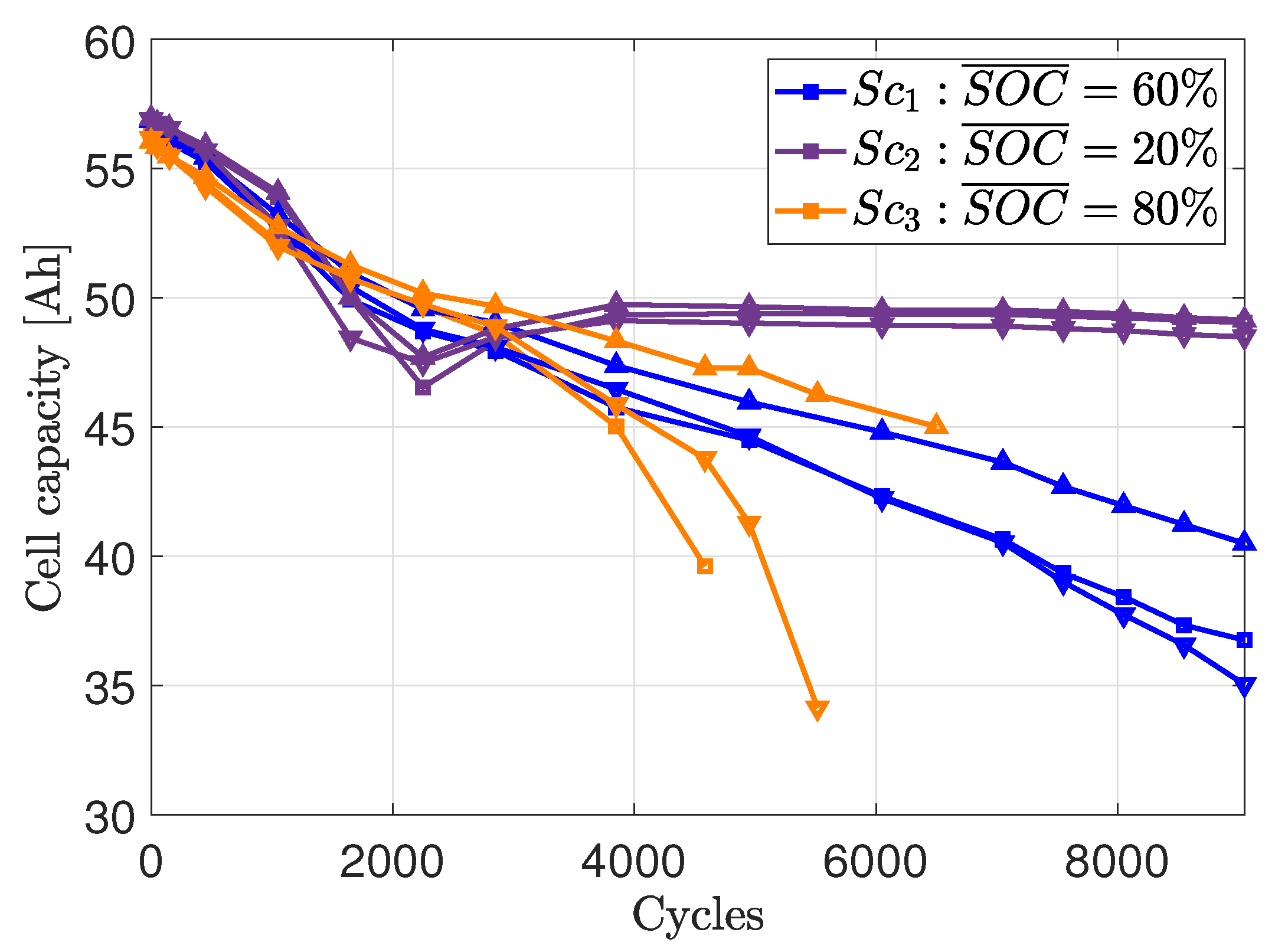
For the experimental validation of the method introduced one of the cell was fully charged and subsequently discharged to determine the available cell capacity. In order to minimize the influence of the cell impedance, a constant-current–constant-voltage (CCCV) protocol was used for both charging and discharging. The CV phases were held until the current dropped below 50 m A . In the CC phase, 25 A were applied during charging and 50 A during discharging. According to the determined capacity the cell was then charged with a constant current of 25 A to certain SOC values (20/40/60/80%). After reaching the desired SOC level, the current was set to zero. The relaxation of the voltage was recorded in high resolution with a sampling rate of 2 M Hz in the first six seconds after the load jump. After six seconds, the sampling rate was reduced down to 1 Hz and the voltage relaxation recorded for 4 h .
The pulse tests were followed by EIS measurements. Galvanostatic excitation with an amplitude of 3 A was applied. The frequency was varied in the range from 50 k Hz to 0.5 m Hz . For frequencies above 100 Hz , 16 measurements per decade were carried out, otherwise only eight were performed. According to Barai et al. [30] the relaxation phase of the previous pulse test is long enough to meet stationary conditions.

3.2. Aging Study

As part of the aging study, the LIBs were cycled under certain operating conditions that are within the manufacturer’s cell specifications. A total of three aging scenarios were carried out, with the average SOC value being varied between the individual scenarios. With the exception of the charging current and the state of charge, the other operating conditions like the depth of discharge (DOD) (30%) and the discharge current ( 1.6 C) were set to be the same for all scenarios. Table 2 gives an overview about the deviating operating conditions for each scenario.
The SOC range of each scenario was set in such a way that, according to [31], different degrees of capacity depletion and deterioration of the individual electrodes could be expected. The aging study thus enables an assessment of whether the sensitivity of the introduced method is sufficient to determine aging mechanisms qualitatively or even quantitatively.
Before starting the cycling, a checkup was carried out for each cell in order to determine the initial cell parameters. During the cycling of the cells, the long-term tests were occasionally interrupted and further checkups were carried out. The checkup procedure contains a CCCV capacity measurement. In addition, at 20/40/60 and 80% a pulse test and an EIS measurement are performed, following the procedure described in Section 3.1. However, the maximum sampling rate during the pulse test is limited to 10 Hz , which is more realistic for online applications such as battery management systems.

4. Results

4.1. Experimental Validation

In this section, the results of the pulse tests and the EIS measurements of the experimental validation are shown and evaluated.
Figure 4 depicts the recorded cell voltage during the relaxation at 20%. In addition to the originally measured signal, the moving average of the signal is given in order to be able to assess the accuracy of the reconstructed signal. It can be stated that the deviation between the reconstructed and the averaged signal over the entire range under consideration is less than 0.5 m V .
The high measurement resolution reveals the inductive behavior of the cell voltage. Due to the inductance, the voltage over the cell connectors and current collectors drop to negative values immediately after the load jump. For less than 0.1 m s , the voltage rises again as the voltage across the inductive components drops quickly. Therefore, the voltage measurements for t < 0.1 m s have been omitted, as electrochemical processes (time constants of usually larger than 1 m s ) are of interest for this study. However, it is pointed out that the inductive behavior can also be simulated by expanding the matrix A (Equation (9)) by the mathematical description of several parallel circuits of ohmic resistance and inductance (RL-elements).
Equation (19) is used to calculate the impedance of the cell for the pulse test at 20% percent. For better comparability with the spectrum measured directly after the pulse test, Figure 5a,b show the imaginary and real parts of both spectra over frequency.
Figure 5a shows that the imaginary part coincides with frequencies below 50 Hz . Due to the limited measuring range, only impedances at frequencies above 0.5   m Hz can be specified for the measured spectrum.
The plot of the real part of the impedance in Figure 5b provides similar insights. The course of the reconstructed spectrum deviates at high frequencies, but follows the measured spectrum at frequencies of ≤ 5 Hz .
The increasing deviations at > 5 Hz can be explained by the Butler–Volmer kinetics. The current excitation at relaxation period was set to zero, while the excitation during the direct measurement of the impedance was set between − 3 A and 3 A . According to the Butler–Volmer equation, the kinetics of charge transfer processes are not linear. Thus, due to increasing charge transfer resistances, the potential response does not decrease linearly with the current excitation [32]. In addition, it has been experimentally proven in some publications that the relaxation time, which differs between the pulse test and the EIS, influences the charge transfer resistances [30,32]. It is known that charge transfer processes at the anode [4,15] and at the cathode [5,33] occur at moderate frequencies of 1–100 Hz . The deviations at frequencies of 5–100 Hz between pulse test and EIS were therefore to be expected.
The ranges of the spectrum at frequencies above 100 Hz could not be adequately reconstructed because the optimization function is limited to resistive–capacitive elements. The impedance values measured at over 100 Hz were therefore discarded and not plotted in Figure 5.
Figure 6 shows the DRT obtained from time domain data and the DRT determined from frequency domain data. The resolution of the DRT from time domain data is twice as high. Therefore, the heights of peaks in one DRT cannot be compared directly with those in the other DRT. In order to compare the polarization contributions of the identified processes, the sum of all polarization contributions within a peak must be determined instead. When calculating the polarization contributions for the first (peak at smallest time constant) to fifth peak, the same orders of magnitude result for the respective peak for both DRTs. In addition, both DRTs show that the contribution of the first and fifth peaks are greatest, followed by the fourth and second peaks. The third peak has a comparatively small contribution in both DRTs.
Both distributions reveal four relevant processes with time constants in the range of 2 · 10 3 s < τ < 2 · 10 0 s . According to f T = 1 2 · π τ , these time constants approximately correspond to frequencies between 0.1 Hz and 100 Hz . Processes in this frequency range were assigned to charge transfer [4,5,15,33] and surface films of the electrodes [4,34]. Due to the Butler–Volmer kinetics, time constants and polarization contributions differ between the two distributions, which explains the discrepancy that occurs in the first four peaks.
For time constants > 10 s , the DRT obtained from time domain data shows a comparatively better resolution of the processes. The DRT based on frequency domain data only indicates a single process for time constants between 10 and 1000 s . In contrast, the DRT obtained through time domain data reveals the existence of three different processes. In addition, time constants that are two orders of magnitude higher can be resolved. If the spectrum is recorded via EIS, the measurement takes more than a day to resolve large time constants. The evaluation of pulse data with the method introduced can therefore be advantageous for examining processes with large time constants such as solid state diffusion.

4.2. Aging Study

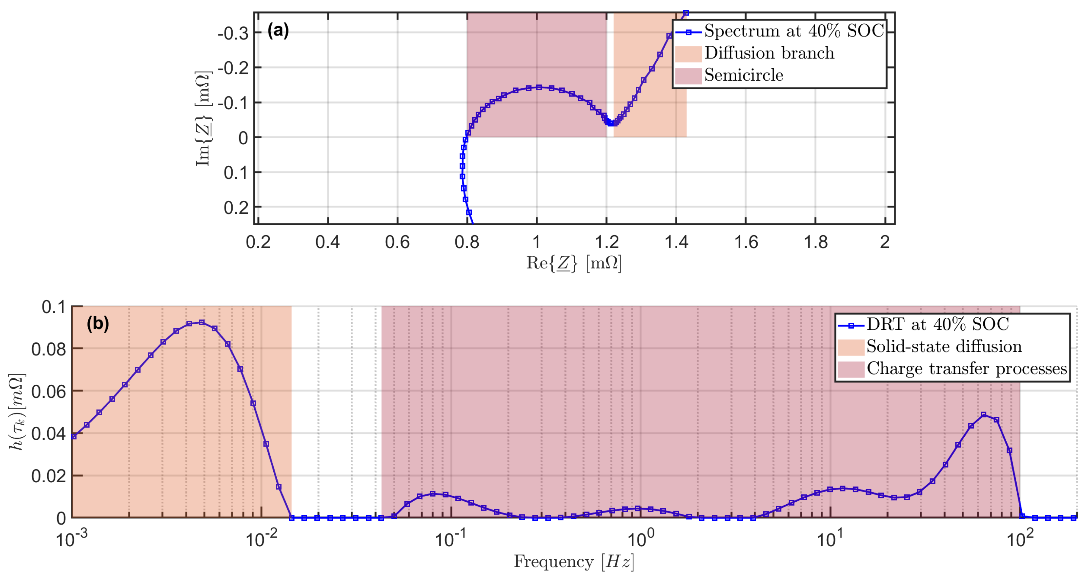
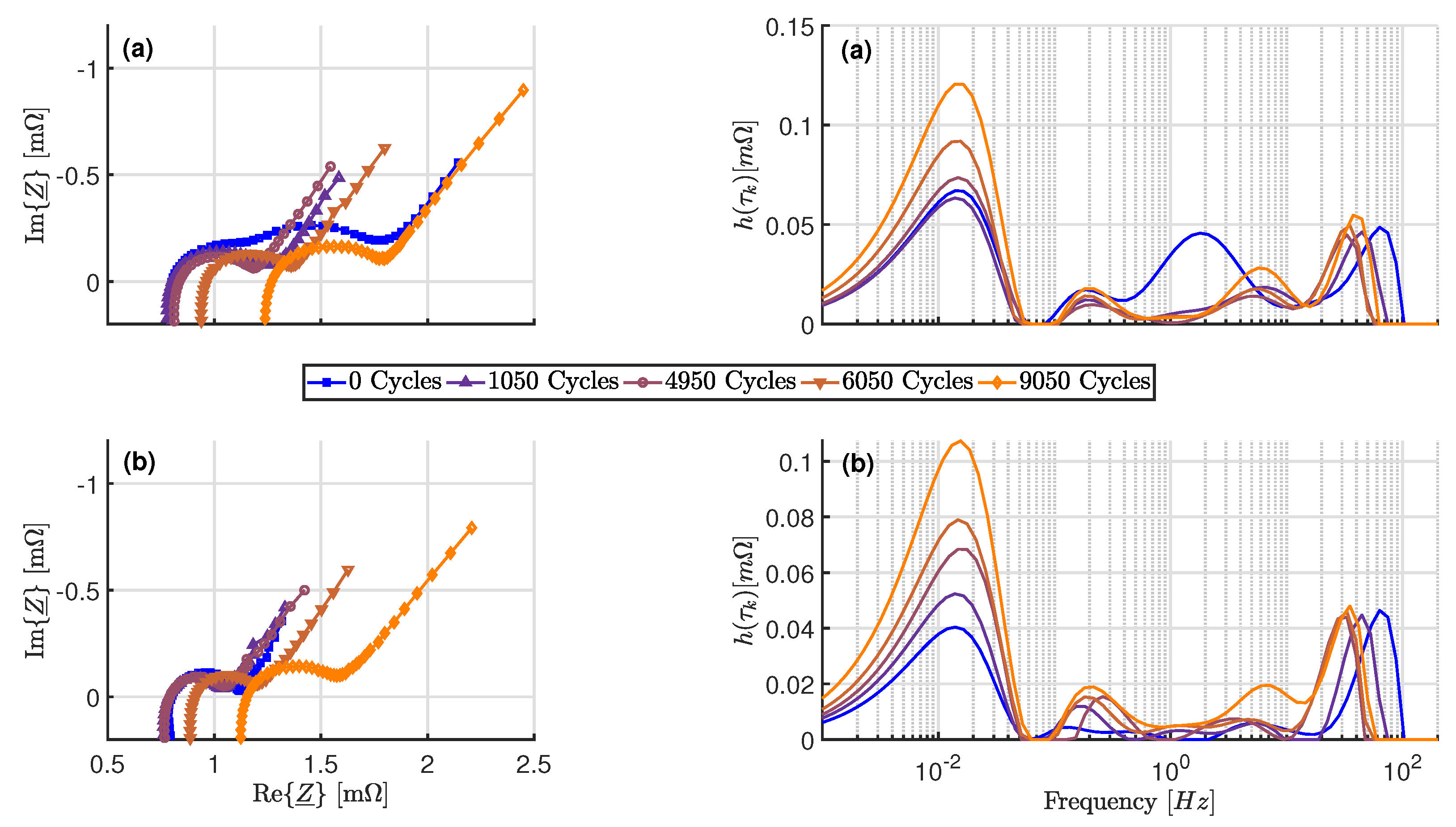
4.2.1. EIS Measurement Evaluation

In Figure 7 shows the measured spectra and the corresponding DRT against frequency of an examined cell as well as the development during aging. The measurements from one cell from aging scenario S c 1 were selected for the exemplary representation. The upper diagrams show the values determined at 20% and the lower part at 80% SOC.
In the Nyquist diagram, two major changes can be seen as the cell ages:
  • An increase of the internal cell resistance R i during aging (Shifting of the zero crossing of the imaginary axis to higher real parts)
  • Disappearance of the second semicircle at 20% SOC during the first 1050 cycles of the long-term test
According to the second bullet point, the DRT at 20% reveals distinct changes in the polarization contribution and the time constant for a process at moderate frequencies. This peak can be assigned to the second semicircle in the spectrum because it occurs particularly when the SOC is low and the cell is new. As already mentioned, this peak can be assigned to a charge transfer process due to the range of the time constant.
In contrast to the observation of the spectra, the analysis of the DRT shows a slight increase in the contribution of this process during the last cycles. Furthermore, slight increases in the polarization of the charge transfer processes are visible at moderate frequencies and 80%. In addition, small changes in the parameters of the process with the smallest time constant are visible, but they do not follow a clear trend. Due to the frequency range, this process can be assigned to the transfer through the SEI of the anode [4,34].
For frequencies < 0.1 Hz , a single process is visible. At low SOC, the polarization of the process remains almost constant during the first 4950 cycles. After the first 4950 cycles, a continuous increase can be observed. At 80% SOC, this continuous increase begins with the start of the long-term test.
The mentioned changes in the process parameters were recognizable for all cells, except for the increase in polarization contribution at low frequencies. This behavior was not pronounced in the cells of scenario S c 2 . Changes of the process parameters were made at a similar rate within a scenario. However, there were deviations in the rate of change between the scenarios, especially with regard to the increase in polarization contribution at frequencies below 0.1 Hz .

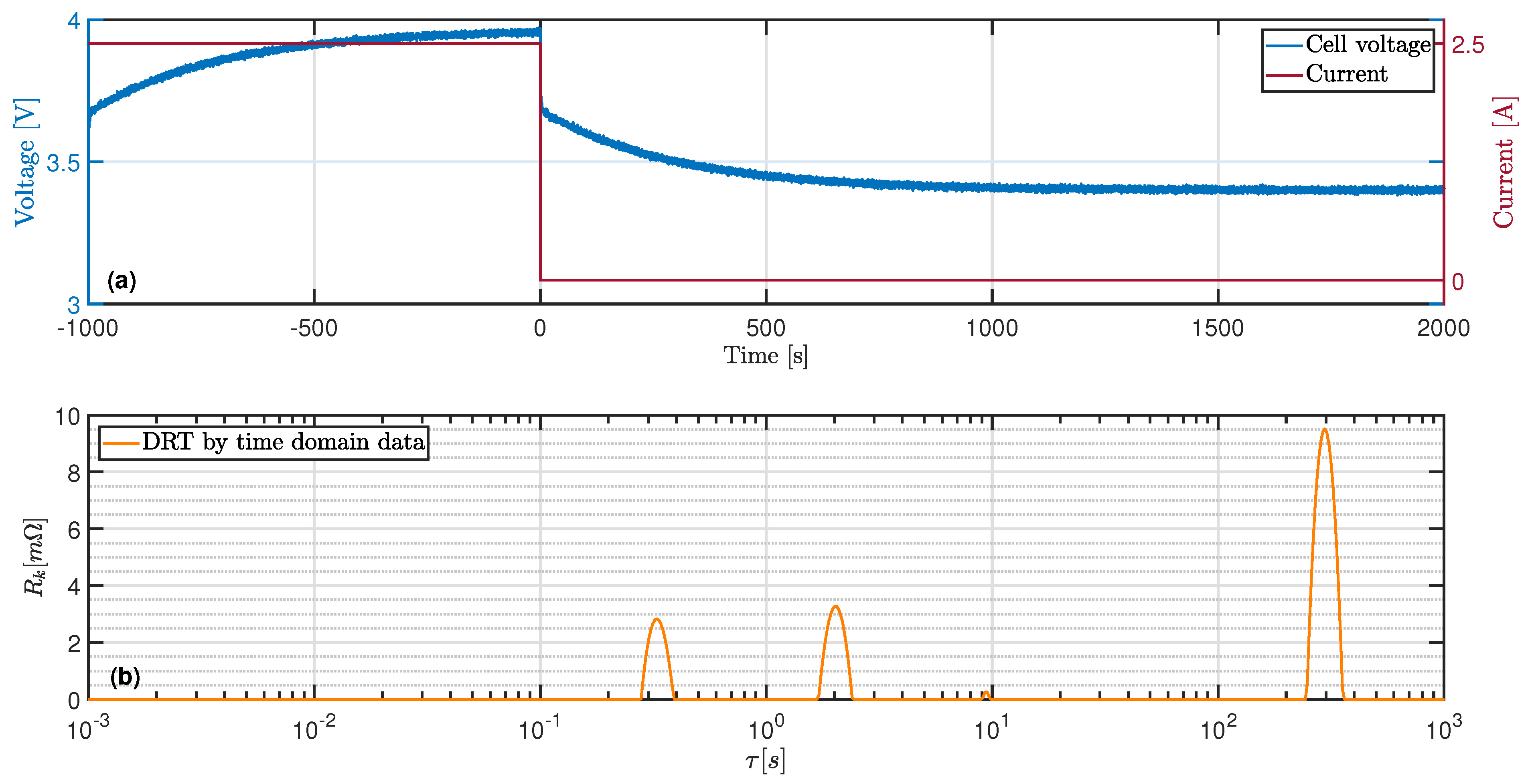
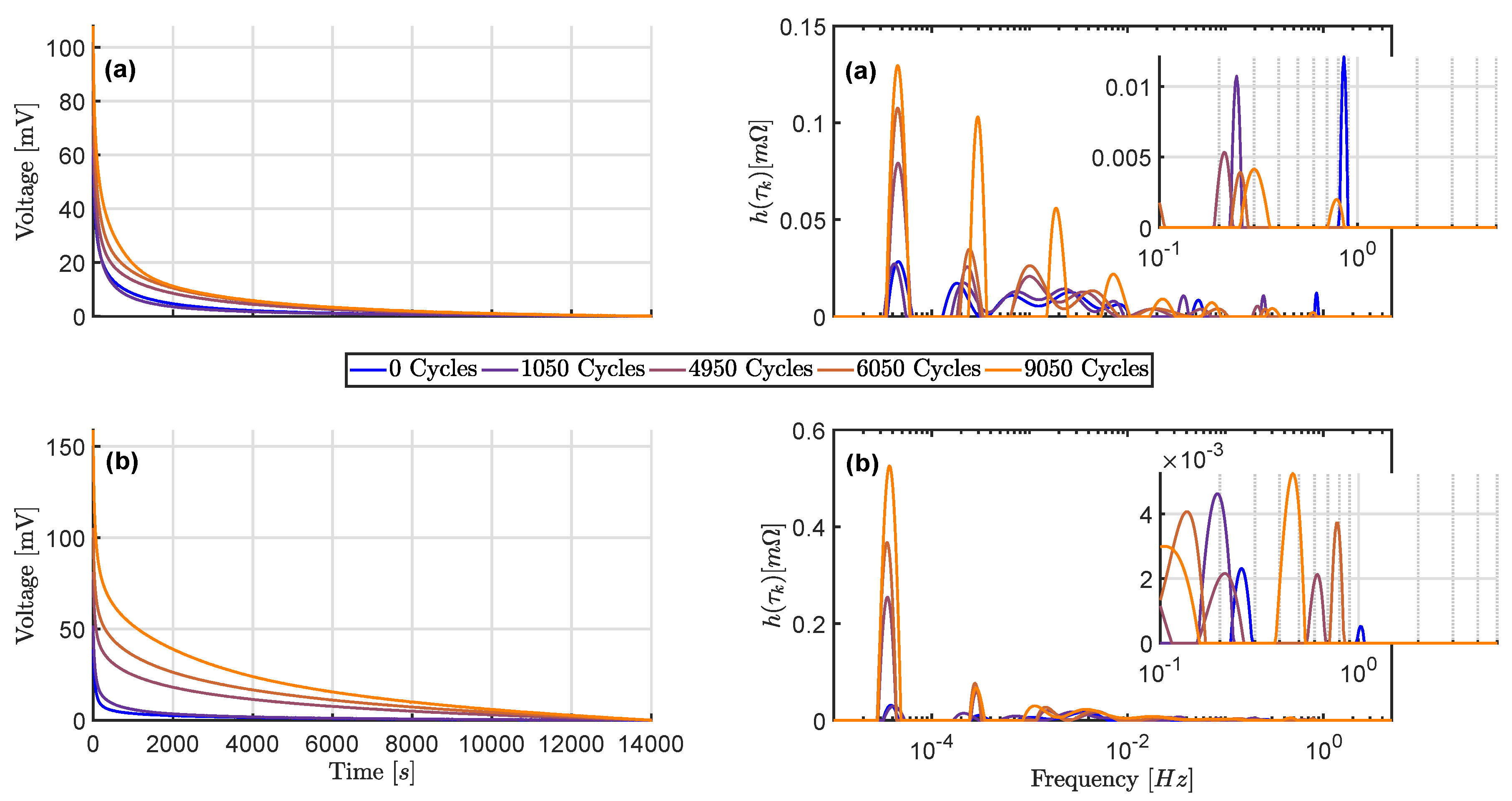
4.2.2. Pulse Test Evaluation

Figure 8 shows the cell voltage course during the relaxation period and the DRT derived from the time domain data. Again, the values at 20% (upper graphs) and 80% SOC (lower graphs) are given and the same cell as in Section 4.2.1 is evaluated.
The voltage courses show a slowdown of the relaxation process as aging progresses. The DRT derived by the time domain data reveals changing parameters of processes with large time constants as the reason. A strong increase of polarization contributions can be observed for low frequencies. Compared to the DRT obtained from frequency domain data, not only a more pronounced increase can be observed. In addition, more processes with large time constants can be identified, since the DRT can also be specified for frequencies that are lower than 1 m Hz .
According to Equation (10), the DRT only provides representative values for the frequencies ≤ 5 Hz . The DRT is cut off accordingly for frequencies above 5 Hz . The process with the smallest time constant shown in Figure 7 (assigned to the SEI) is therefore not visible.
The disappearance of a polarization contribution of a process at moderate frequencies and 20% SOC can be confirmed. The number of processes in the range of moderate frequencies between 0.1 and 5 Hz corresponds to the number determined on the basis of frequency domain data. However, the greater spread of the time constants and the polarization with no discernible trend shows that due to the lower sampling frequency the accuracy is too low to reliably quantize the parameters of the identified processes at moderate frequencies.

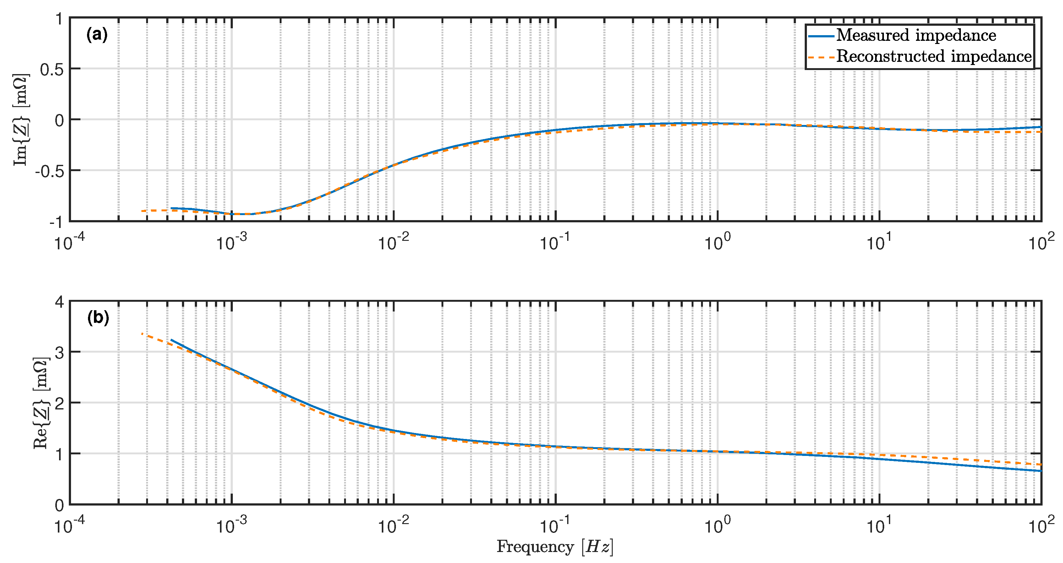
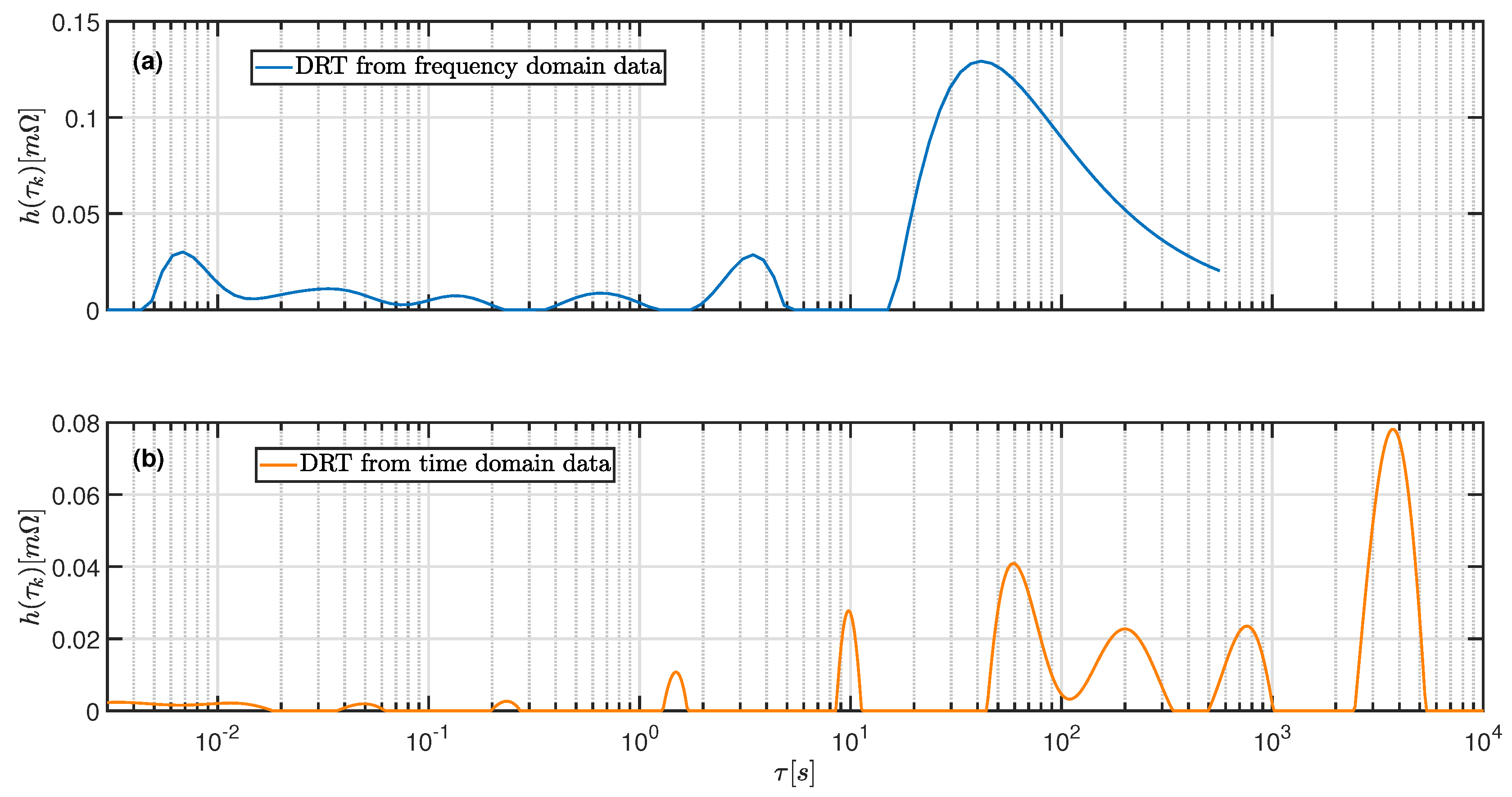
4.2.3. Comparison of DRT by Time and Frequency Domain Data

The results of the experimental studies can be summarized as follows:
  • Processes with characteristic time constants that do not meet Equation (12) cannot be identified with the set sampling rate using the time domain data alone.
  • Already with a maximum sampling rate of 10 Hz , which is realistic for online applications, the DRT by time domain data can be used to identify charge transfer processes and to provide a qualitative description. However, the change in process parameters during aging can only be traced to a limited extent.
  • Quantitative statements for charge transfer processes, even if higher sampling rates are used, differ between the two methods due to the Butler–Volmer kinetics. In fact, due to the strongly non-linear excitations in real applications, the better transferability of the results obtained from frequency domain data is questionable.
  • The DRT based on time domain data is more sensitive for processes with large characteristic time constants such as solid state diffusion.
  • When using frequency domain data, either longer measuring periods are required or the measuring range is limited to higher frequencies, since different frequencies have to be excited successively during EIS.

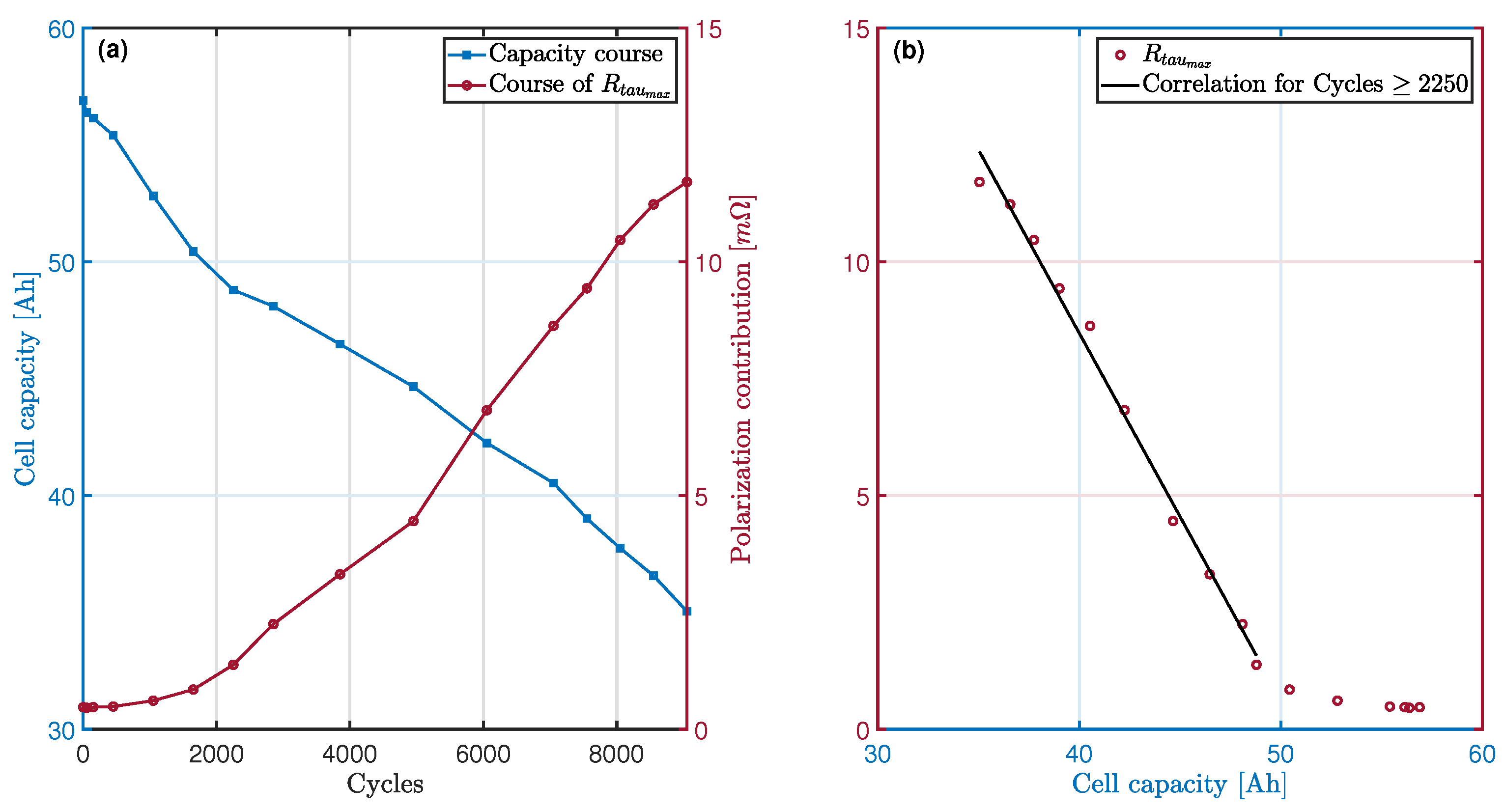
4.2.4. Correlation of the Capacity and the Identified Process Parameters

Figure 9a shows the capacity course during the aging of a cell and the corresponding polarization contribution of the process with the largest time constant, which is determined by time domain data at 60% SOC. The polarization contribution is referred to below as R t a u m a x . The results belong to the cell that has already been evaluated in the previous Section 4.2.1 and Section 4.2.2.
For a better overview of the correlation between the two parameters, the development of R t a u m a x is plotted over the capacity. A strong negative correlation can be found for ≥2250 cycles. During the first cycles, the increase in polarization in relation to the capacity fade is less pronounced. Regardless of which scenario, a significantly weaker increase in R t a u m a x could be confirmed for all cells at the beginning of the aging tests. Thus, the average correlation coefficients C c o e f f for each scenario and for the cycles ≥2250 are given in Table 3.
Taking into account the measurement data only for cycles ≥2250, a Pearson correlation coefficient of ≥98% can be specified for scenarios S c 1 and S c 3 , which indicates a high negative correlation between the two parameters. For scenario S c 2 , the correlation is weaker, but still noticeable.
Figure 10 shows the capacity courses over the cycles for all cells examined.
For scenario S c 2 , a recovery of cell capacity can be seen. After 2250 cycles, the capacity remains relatively constant at around 48 A h . Because of the flat curve, the accurate correlation is more difficult to determine because of the corresponding small changes in polarization R t a u m a x are difficult to detect. This could be one reason why the correlation coefficient is lower in scenario S c 2 .
To further investigate the reasons for the lower correlation coefficient, the correlation between the capacity of the anode and the polarization R t a u m a x was determined. The determination of the loss of active material at the anode (LAMAn) on the basis of the non-invasive measurements during the checkups was carried out in [27]. The correlation between the LAMAn and R t a u m a x was ≥ 96% for each cell of scenario S c 1 from cycle 0 to 9050. Taking into account the uncertainties in the estimation of the LAMAn, 96% is a high value and it can be stated that the increase in R t a u m a x is associated with the LAMAn. For all cells of scenario S c 1 the decrease in capacity at the anode was more pronounced compared to the cells of S c 2 . Gantenbein et al. has already experimentally confirmed a higher LAMAn for cells that were cycled at SOC levels above 65%, while the LAMAn for cells that were cycled below 45% was neglible [31]. The lower LAMAn provides a further reason for the lower correlation in S c 2 and the lower capacity fade during aging. For the cells of S c 3 , the LAMAn after 3850 cycles could not be determined due to a change in the electrode balance [27]. According to the results of [31] a comparatively high LAMAn is to be expected. This statement is supported by the correlation factor determined for scenario S c 3 (see Table 3).
In contrast to the correlation to the cell capacity (see Figure 9), the linear relationship between LAMAn and increase in R t a u m a x is visible from the first few cycles of the long-term test. It is known from the literature that the cell capacity can be limited by different degradation mechanisms in different aging stages of a LIB (e.g., [35,36]). In a previous publication, the loss of lithium inventory (LLI) was identified as the main aging mechanism during the first few cycles of the aging study described [27]. The LAMAn becomes the limiting factor for the capacity of the cells of scenarios S c 1 and S c 3 after 2250 cycles. Therefore, a correlation between the cell capacity and the R t a u m a x only becomes visible after 2250 cycles. It is thus assumed that the correlation between the cell capacity and R t a u m a x originates from the correlation of LAMAn and R t a u m a x .

5. Discussion

In the context of the aging study, the method introduced has proven to be advantageous for investigating processes with time constants in the range of minutes to hours. In addition to the more precise resolution of the low-frequency processes compared to the DRT, which is derived from frequency domain data, the time required for the measurements is significantly lower. Besides higher resolution and lower time efforts, the steady state criterion with regard to the SOC is not violated during the relaxation period. In order to avoid a change in the SOC during the EIS at low frequencies, the excitation current must be limited, which leads to a comparatively poor signal-to-noise ratio.
However, high sampling rates are required in order to investigate frequency-dependent processes with characteristic time constants in the range of a few seconds or even milliseconds such as charge transfer and SEI. According to the Shannon theorem, time constants in the range of milliseconds should theoretically be able to be evaluated with a sampling rate of 10 Hz , which is realistic for an online application. In contrast to this, the aging study has shown that only the parameters of processes with time constants of almost two decades higher ( τ 1.6 s ) can be quantified with sufficient accuracy using the aforementioned sampling rate. In many applications, and especially in most online applications, the method presented is therefore limited to the aging monitoring of processes with time constants in the range of seconds to several hours, such as solid state diffusion.
Therefore, for applications in which both pulse tests and EIS are possible, a combined use of both techniques is proposed. By merging the impedance data obtained through time and frequency domain data as suggested by [19], the impedance spectrum and DRT can be determined for a wide frequency range.
Using the DRT derived from the time domain data, a correlation between the polarization contribution and LAMAn could be determined at low frequencies around 35 μ Hz . Due to the limited frequency range of the EIS, this connection could not be established using the frequency domain data. A correlation between a degradation mechanisms and the impedance of LIBs could already be established in earlier studies. In a comprehensive experimental study, the correlations between kinetic parameters of an LIB and degradation mechanisms could be derived [1]. Recently, a correlation between low frequency impedance and the LLI was found in [24] and Schindler et al. [37] confirmed a correlation between the low frequency impedance and LAM. Using cell kinetics to gain insights into the degradation mechanisms is beneficial because measuring impedances at high and moderate frequencies is fast compared to deriving the mechanisms by recording open circuit voltage curves [1]. However, EIS measurements suffer from long measurement durations for low-frequency impedances and a lack of availability in most state-of-the-art online applications. In contrast, relaxation periods occur in every online application. As a result, the introduced method enables a time-effective investigation that can be used online in order to obtain the relevant parameters of the processes with large time constants and thus enable an online estimate of the degradation mechanisms.
It is known that LIBs can suffer from accelerated capacity loss towards the end of life due to lithium plating originally caused by a lack of anodic material [35,36]. For online applications, an early detection of an increasing capacity reduction and lithium plating is of great importance for the reliability and safety of LIBs. Many publications like [38] have therefore dealt with the prediction of the sudden reduction in capacity. As a further outcome of this study, the correlation found could be used to identify an advanced LAMAn online and thus the risk of lithium plating and the resulting rapid loss of capacity at an early stage.
In summary, this work showed that the evaluation of the voltage relaxation after a current pulse is suitable for investigating the kinetic parameters of a LIB even without prior knowledge of the polarization processes involved. The DRT obtained from the time domain data offers a time-effective determination of processes with large characteristic time constants and enables the parameters to be estimated online. The correlations found provide insights into the degradation mechanisms both offline and online and thus support the future battery design and enable optimization of the operating strategies. The findings about the early detection of a potential risk of lithium plating are available for subsequent studies and contribute to improving the reliability and safety of LIBs.
In a future step, Post-Mortem analyses will be carried out to directly quantify the LAMAn and validate the assumptions made. In addition, the transferability of the results to other cell chemistries and formats must be checked.

Author Contributions

Conceptualization, E.G.; methodology, E.G.; software, E.G.; validation, E.G.; formal analysis, E.G.; investigation, E.G.; resources, J.K.; data curation, E.G.; writing—original draft preparation, E.G.; writing—review and editing, J.K. and E.G.; visualization, E.G.; supervision, J.K.; project administration, E.G.; funding acquisition, J.K. All authors have read and agreed to the published version of the manuscript.

Funding

This research was funded by Bundesministerium für Bildung und Forschung grant number 16EMO0262 (SiCWell).

Institutional Review Board Statement

Not applicable.

Informed Consent Statement

Not applicable.

Data Availability Statement

Not applicable.

Conflicts of Interest

The authors declare no conflict of interest. The funders had no role in the design of the study; in the collection, analyses, or interpretation of data; in the writing of the manuscript, or in the decision to publish the results.

Abbreviations

The following abbreviations are used in this manuscript:
DRTDistribution of relaxation times
LIBLithium-ion battery
EISElectrochemical impedance spectroscopy
EVElectric vehicle
OCVOpen circuit voltage
SEISolid electrolyte interface
FFTFast Fourier transform
ECMEquivalent circuit model
SOCState of charge
NMCNickel-manganese-cobalt-oxide
CCCVconstant-current-constant-voltage
DODDepth of discharge
LAMAnLoss of active material at the anode
LLILoss of lithium inventory

References

  1. Pastor-Fernández, C.; Uddin, K.; Chouchelamane, G.H.; Widanage, W.D.; Marco, J. A Comparison between Electrochemical Impedance Spectroscopy and Incremental Capacity-Differential Voltage as Li-ion Diagnostic Techniques to Identify and Quantify the Effects of Degradation Modes within Battery Management Systems. J. Power Sources 2017, 360, 301–318. [Google Scholar] [CrossRef]
  2. Pastor-Fernández, C.; Yu, T.F.; Widanage, W.D.; Marco, J. Critical review of non-invasive diagnosis techniques for quantification of degradation modes in lithium-ion batteries. Renew. Sustain. Energy Rev. 2019, 109, 138–159. [Google Scholar] [CrossRef]
  3. Schindler, S.; Bauer, M.; Petzl, M.; Danzer, M.A. Voltage relaxation and impedance spectroscopy as in-operando methods for the detection of lithium plating on graphitic anodes in commercial lithium-ion cells. J. Power Sources 2016, 304, 170–180. [Google Scholar] [CrossRef]
  4. Steinhauer, M.; Risse, S.; Wagner, N.; Friedrich, K.A. Investigation of the Solid Electrolyte Interphase Formation at Graphite Anodes in Lithium-Ion Batteries with Electrochemical Impedance Spectroscopy. Electrochim. Acta 2017, 228, 652–658. [Google Scholar] [CrossRef]
  5. Shafiei Sabet, P.; Warnecke, A.J.; Meier, F.; Witzenhausen, H.; Martinez-Laserna, E.; Sauer, D.U. Non-invasive yet separate investigation of anode/cathode degradation of lithium-ion batteries (nickel–cobalt–manganese vs. graphite) due to accelerated aging. J. Power Sources 2020, 449, 227369. [Google Scholar] [CrossRef]
  6. Schmitt, J.; Maheshwari, A.; Heck, M.; Lux, S.; Vetter, M. Impedance change and capacity fade of lithium nickel manganese cobalt oxide-based batteries during calendar aging. J. Power Sources 2017, 353, 183–194. [Google Scholar] [CrossRef]
  7. Andre, D.; Meiler, M.; Steiner, K.; Wimmer, C.; Soczka-Guth, T.; Sauer, D.U. Characterization of high-power lithium-ion batteries by electrochemical impedance spectroscopy. I. Experimental investigation. J. Power Sources 2011, 196, 5334–5341. [Google Scholar] [CrossRef]
  8. Tröltzsch, U.; Kanoun, O.; Tränkler, H.R. Characterizing aging effects of lithium ion batteries by impedance spectroscopy. Electrochim. Acta 2006, 51, 1664–1672. [Google Scholar] [CrossRef]
  9. Jossen, A. Fundamentals of battery dynamics. J. Power Sources 2006, 154, 530–538. [Google Scholar] [CrossRef]
  10. Tuncer, E.; Macdonald, J.R. Comparison of methods for estimating continuous distributions of relaxation times. J. Appl. Phys. 2006, 99, 074106. [Google Scholar] [CrossRef] [Green Version]
  11. Saccoccio, M.; Wan, T.H.; Chen, C.; Ciucci, F. Optimal Regularization in Distribution of Relaxation Times applied to Electrochemical Impedance Spectroscopy: Ridge and Lasso Regression Methods - A Theoretical and Experimental Study. Electrochim. Acta 2014, 147, 470–482. [Google Scholar] [CrossRef]
  12. Wan, T.H.; Saccoccio, M.; Chen, C.; Ciucci, F. Influence of the Discretization Methods on the Distribution of Relaxation Times Deconvolution: Implementing Radial Basis Functions with DRTtools. Electrochim. Acta 2015, 184, 483–499. [Google Scholar] [CrossRef]
  13. Boukamp, B.A.; Rolle, A. Analysis and Application of Distribution of Relaxation Times in Solid State Ionics. Solid State Ion. 2017, 302, 12–18. [Google Scholar] [CrossRef]
  14. Danzer, M.A. Generalized Distribution of Relaxation Times Analysis for the Characterization of Impedance Spectra. Batteries 2019, 5, 53. [Google Scholar] [CrossRef] [Green Version]
  15. Hahn, M.; Schindler, S.; Triebs, L.C.; Danzer, M.A. Optimized Process Parameters for a Reproducible Distribution of Relaxation Times Analysis of Electrochemical Systems. Batteries 2019, 5, 43. [Google Scholar] [CrossRef] [Green Version]
  16. Ivers-Tiffée, E.; Weber, A. Evaluation of electrochemical impedance spectra by the distribution of relaxation times. J. Ceram. Soc. Jpn. 2017, 125, 193–201. [Google Scholar] [CrossRef] [Green Version]
  17. Manikandan, B.; Ramar, V.; Yap, C.; Balaya, P. Investigation of physico-chemical processes in lithium-ion batteries by deconvolution of electrochemical impedance spectra. J. Power Sources 2017, 361, 300–309. [Google Scholar] [CrossRef]
  18. Alavi, S.; Birkl, C.R.; Howey, D.A. Time-domain fitting of battery electrochemical impedance models. J. Power Sources 2015, 288, 345–352. [Google Scholar] [CrossRef]
  19. Klotz, D.; Schönleber, M.; Schmidt, J.P.; Ivers-Tiffée, E. New approach for the calculation of impedance spectra out of time domain data. Electrochim. Acta 2011, 56, 8763–8769. [Google Scholar] [CrossRef]
  20. Karger, A.; Wildfeuer, L.; Maheshwari, A.; Wassiliadis, N.; Lienkamp, M. Novel method for the on-line estimation of low-frequency impedance of lithium-ion batteries. J. Energy Storage 2020, 32, 101818. [Google Scholar] [CrossRef]
  21. Schröer, P.; Khoshbakht, E.; Nemeth, T.; Kuipers, M.; Zappen, H.; Sauer, D.U. Adaptive modeling in the frequency and time domain of high-power lithium titanate oxide cells in battery management systems. J. Energy Storage 2020, 32, 101966. [Google Scholar] [CrossRef]
  22. Zou, C.; Zhang, L.; Hu, X.; Wang, Z.; Wik, T.; Pecht, M. A review of fractional-order techniques applied to lithium-ion batteries, lead-acid batteries, and supercapacitors. J. Power Sources 2018, 390, 286–296. [Google Scholar] [CrossRef] [Green Version]
  23. Schmidt, J.P.; Berg, P.; Schönleber, M.; Weber, A.; Ivers-Tiffée, E. The distribution of relaxation times as basis for generalized time-domain models for Li-ion batteries. J. Power Sources 2013, 221, 70–77. [Google Scholar] [CrossRef]
  24. Zhu, J.; Dewi Darma, M.S.; Knapp, M.; Sørensen, D.R.; Heere, M.; Fang, Q.; Wang, X.; Dai, H.; Mereacre, L.; Senyshyn, A.; et al. Investigation of lithium-ion battery degradation mechanisms by combining differential voltage analysis and alternating current impedance. J. Power Sources 2020, 448, 227575. [Google Scholar] [CrossRef]
  25. Hentunen, A.; Lehmuspelto, T.; Suomela, J. Time-Domain Parameter Extraction Method for Thévenin-Equivalent Circuit Battery Models. IEEE Trans. Energy Convers. 2014, 29, 558–566. [Google Scholar] [CrossRef]
  26. Xiaosong, H.; Fengchun, S.; Yuan, Z.; Huei, P. Online estimation of an electric vehicle Lithium-Ion battery using recursive least squares with forgetting. In Proceedings of the 2011 American Control Conference, San Francisco, CA, USA, 29 June–1 July 2011; pp. 935–940. [Google Scholar] [CrossRef]
  27. Goldammer, M.S.E.; Kowal, J. Investigation of degradation mechanisms in lithium-ion batteries by incremental open-circuit-voltage characterization and impedance spectra. In Proceedings of the 2020 IEEE Vehicle Power and Propulsion Conference (VPPC), Gijon, Spain, 18 November–16 December 2020; pp. 1–8. [Google Scholar] [CrossRef]
  28. Tikhonov, A.N.; Goncharsky, A.V.; Hazewinkel, M. Numerical Methods for the Solution of Ill-Posed Problems; Springer: Dordrecht, The Netherlands, 2010. [Google Scholar]
  29. Schindler, S. Diskrete Elektrochemische Modellierung und Experimentelle Identifikation von Lithium-Ionen-Zellen Basierend auf Halbzellpotentialen; Universität Bayreuth: Bayreuth, Germany, 2018. [Google Scholar]
  30. Barai, A.; Widanage, W.D.; Marco, J.; McGordon, A.; Jennings, P. A study of the open circuit voltage characterization technique and hysteresis assessment of lithium-ion cells. J. Power Sources 2015, 295, 99–107. [Google Scholar] [CrossRef]
  31. Gantenbein, S.; Schönleber, M.; Weiss, M.; Ivers-Tiffée, E. Capacity Fade in Lithium-Ion Batteries and Cyclic Aging over Various State-of-Charge Ranges. Sustainability 2019, 11, 6697. [Google Scholar] [CrossRef] [Green Version]
  32. Kindermann, F.M.; Noel, A.; Erhard, S.V.; Jossen, A. Long-term equalization effects in Li-ion batteries due to local state of charge inhomogeneities and their impact on impedance measurements. Electrochim. Acta 2015, 185, 107–116. [Google Scholar] [CrossRef]
  33. Shafiei Sabet, P.; Sauer, D.U. Separation of predominant processes in electrochemical impedance spectra of lithium-ion batteries with nickel-manganese-cobalt cathodes. J. Power Sources 2019, 425, 121–129. [Google Scholar] [CrossRef]
  34. Illig, J.; Ender, M.; Weber, A.; Ivers-Tiffée, E. Modeling graphite anodes with serial and transmission line models. J. Power Sources 2015, 282, 335–347. [Google Scholar] [CrossRef]
  35. Dubarry, M.; Baure, G.; Devie, A. Durability and Reliability of EV Batteries under Electric Utility Grid Operations: Path Dependence of Battery Degradation. J. Electrochem. Soc. 2018, 165, A773–A783. [Google Scholar] [CrossRef]
  36. Anseán, D.; Dubarry, M.; Devie, A.; Liaw, B.Y.; García, V.M.; Viera, J.C.; González, M. Operando lithium plating quantification and early detection of a commercial LiFePO4 cell cycled under dynamic driving schedule. J. Power Sources 2017, 356, 36–46. [Google Scholar] [CrossRef] [Green Version]
  37. Schindler, S.; Danzer, M.A. A novel mechanistic modeling framework for analysis of electrode balancing and degradation modes in commercial lithium-ion cells. J. Power Sources 2017, 343, 226–236. [Google Scholar] [CrossRef]
  38. Fermín-Cueto, P.; McTurk, E.; Allerhand, M.; Medina-Lopez, E.; Anjos, M.F.; Sylvester, J.; dos Reis, G. Identification and machine learning prediction of knee-point and knee-onset in capacity degradation curves of lithium-ion cells. Energy AI 2020, 1, 100006. [Google Scholar] [CrossRef]
Figure 1. (a) Impedance spectra of pristine cell at 40% SOC. (b) Corresponding DRT.
Batteries 07 00036 g001
Figure 2. (a) Simulated cell voltage of a LIB during a pulse test. (b) DRT derived from the voltage relaxation.
Batteries 07 00036 g002
Figure 3. (a) Comparison of simulated and reconstructed voltage during the relaxation period. (b) Comparison of modeled and reconstructed impedance spectrum.
Batteries 07 00036 g003
Figure 4. Pulse test: Voltage relaxation at 20% SOC.
Batteries 07 00036 g004
Figure 5. Comparison of measured and reconstructed impedance at 20% SOC (a) Imaginary part of impedance. (b) Real part of impedance.
Batteries 07 00036 g005
Figure 6. DRT derived from frequency domain data (a) and from time domain data (b).
Batteries 07 00036 g006
Figure 7. Measured impedance spectra and corresponding DRTs over aging (a) At 20% SOC; (b) At 80% SOC.
Batteries 07 00036 g007
Figure 8. Measured voltage relaxation and derived DRTs over aging (a) At 20% SOC; (b) At 80% SOC.
Batteries 07 00036 g008
Figure 9. (a) Capacity course and polarization contribution R t a u m a x vs. cycles. (b) Correlation between capacity and R t a u m a x .
Batteries 07 00036 g009
Figure 10. Capacity course vs. cycles during the long-term cycling.
Batteries 07 00036 g010
Table 1. Comparison of the parameter set of the battery model and the values derived by the DRT.
ParameterCalculated ValueModel ValueRelative Error
R 1 31.5   m Ω 30 m Ω 5%
τ 1 0.328 s 0.3 s 9.2%
R 2 37.5   m Ω 39 m Ω 3.8%
τ 2 2.046 s 1.95 s 4.9%
R 3 116.9   m Ω 117 m Ω <0.1%
τ 3 296.899 s 292.5 s 1.5%
Table 2. Different operating conditions.
Cycling Scenario SOC ¯ [%] I ch [A]
S c 1 6037.5
S c 2 2037.5
S c 3 8018.75
Table 3. Different operating conditions.
Cycling Scenario SOC ¯ [%] C Coeff [%]
S c 1 6099.1
S c 2 2092.8
S c 3 8098.0
Publisher’s Note: MDPI stays neutral with regard to jurisdictional claims in published maps and institutional affiliations.

