Multivariate Monitoring Workflow for Formulation, Fill and Finish Processes


Abstract
:1. Introduction
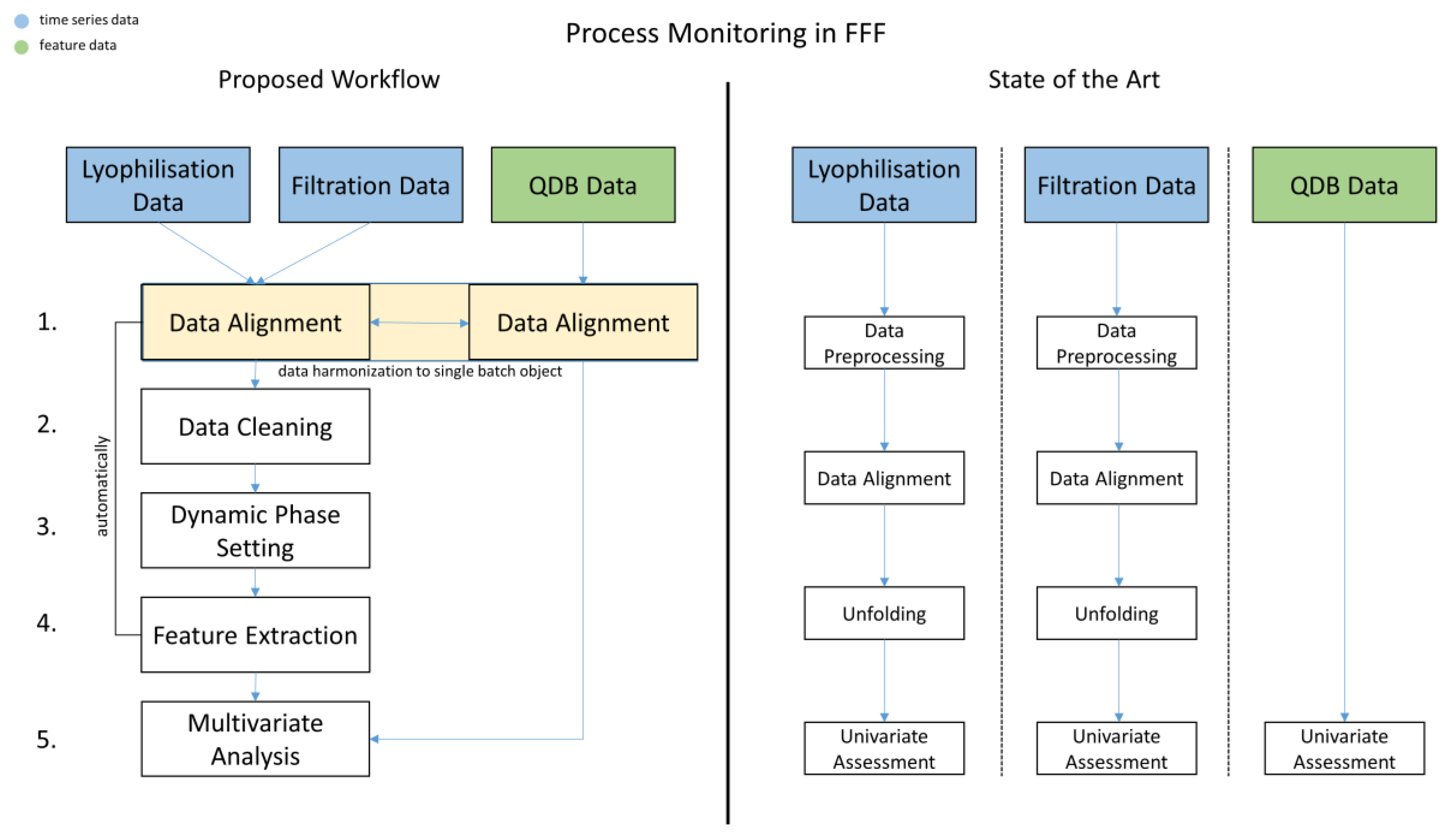
- single-point data (called “feature data”) from intermediates or from Quality Database (QDB) testing (see Figure 1, State of the Art, QDB Data—Univariate Assessment). Examples: lyophilization duration, sterile filtration hold time, amount of various formulation buffer ingredients, etc.
- time-series data during the individual unit operations (see Figure 1, State of the Art, Lyophilization/Filtration Data—Univariate Assessment). Examples: online measurement of product temperature over process time, online measurement of pressure during lyophilization over process time, etc.
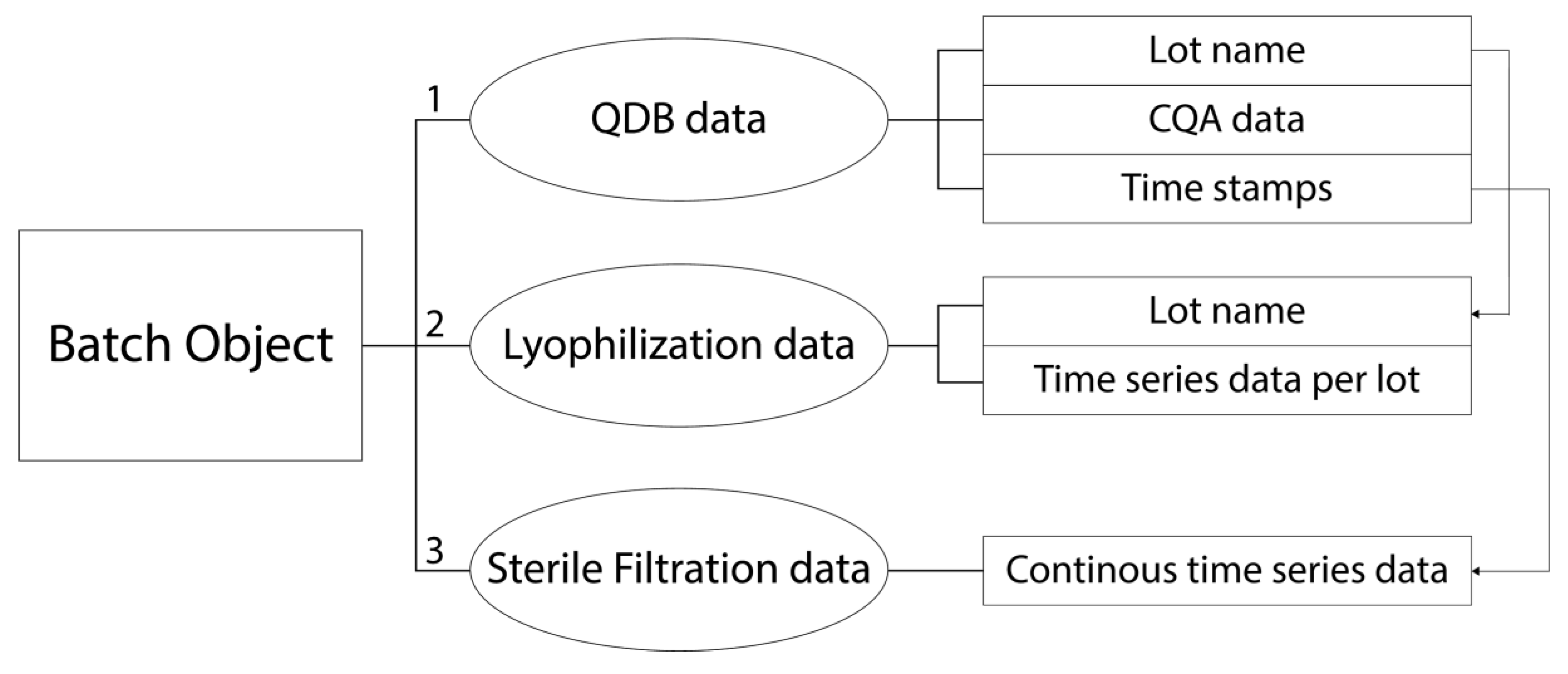
- Assign the available data to the corresponding lots (see Figure 1, Proposed Workflow, Data Alignment).
- Enhance the quality of information by reducing interference signals within the time series (see Figure 1, Proposed Workflow, Data Cleaning).
- Identify process-relevant characteristics of the time-series pattern and leverage for further feature extraction (see Figure 1, Proposed Workflow, Dynamic Phase Setting).
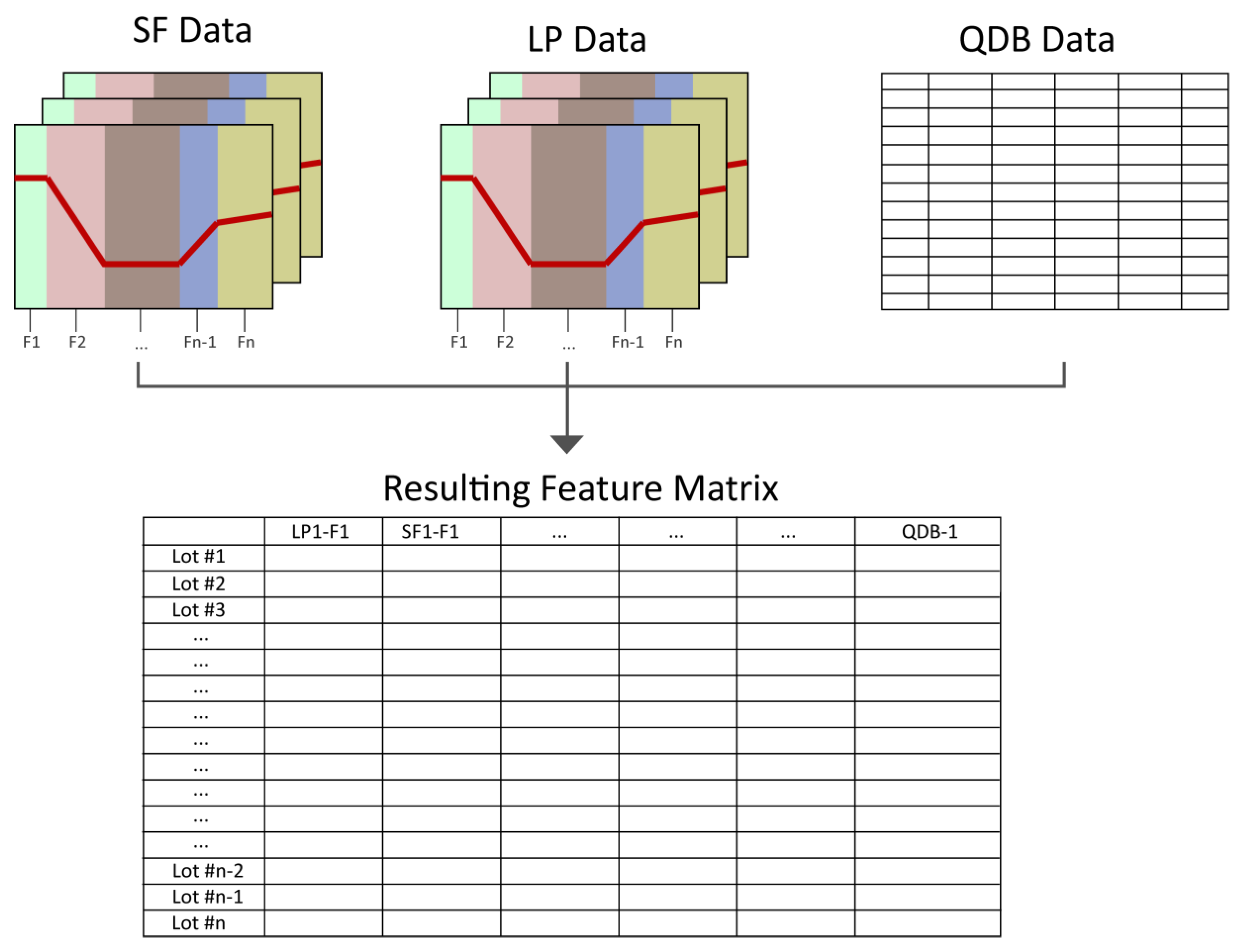
- Create an analytical data set based on the extracted features and combine with already available features (see Figure 1, Proposed Workflow, Feature Extraction).
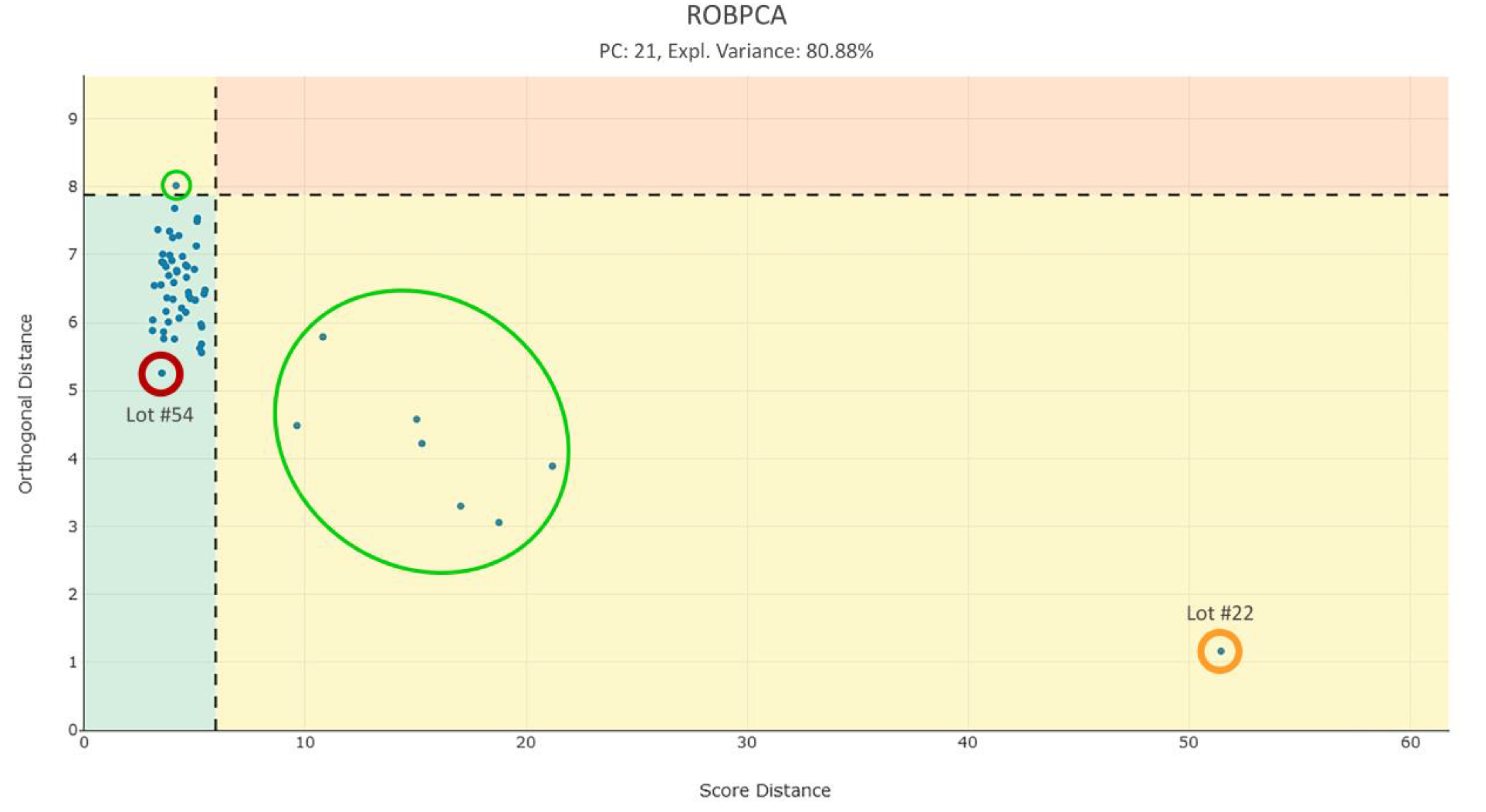
- Perform robust principal component analysis to assess the data set in step 6 (see Figure 1, Proposed Workflow, Multivariate Analysis).
2. Materials and Methods
2.1. Data
2.2. Software
2.3. Statistical Methods
3. Results
3.1. Step 1: Data Alignment
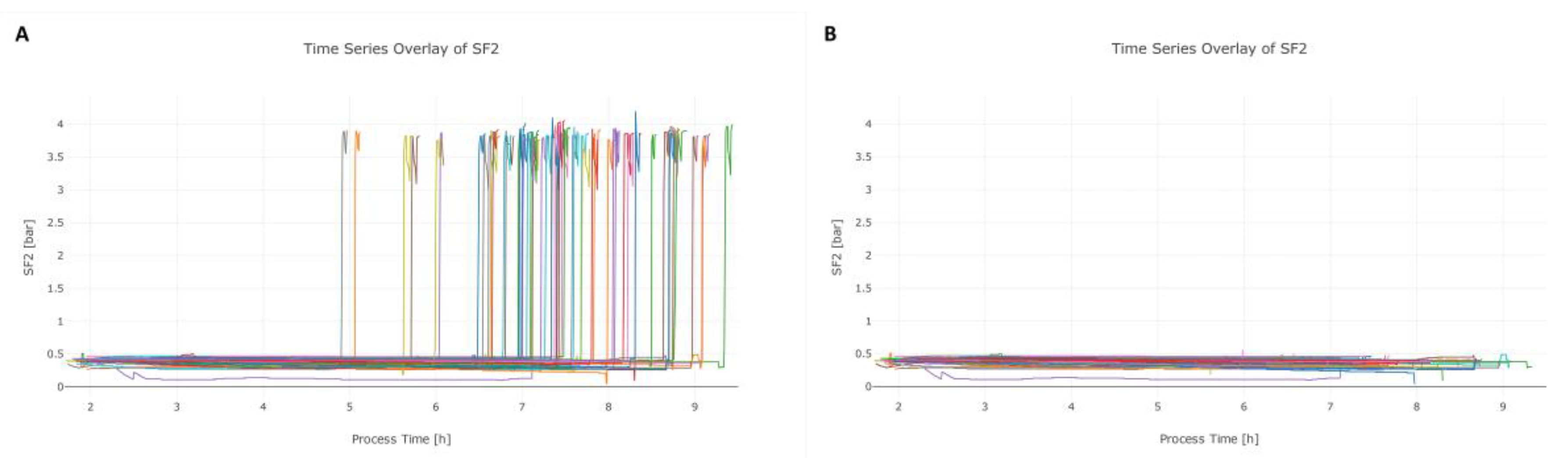
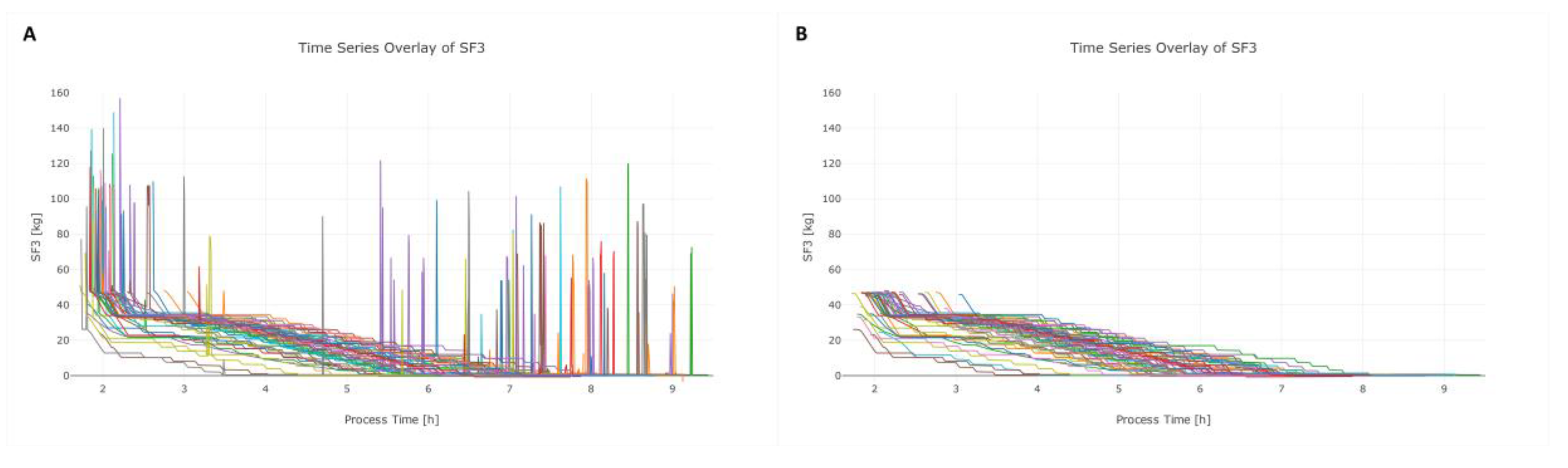
3.2. Step 2: Data Cleaning
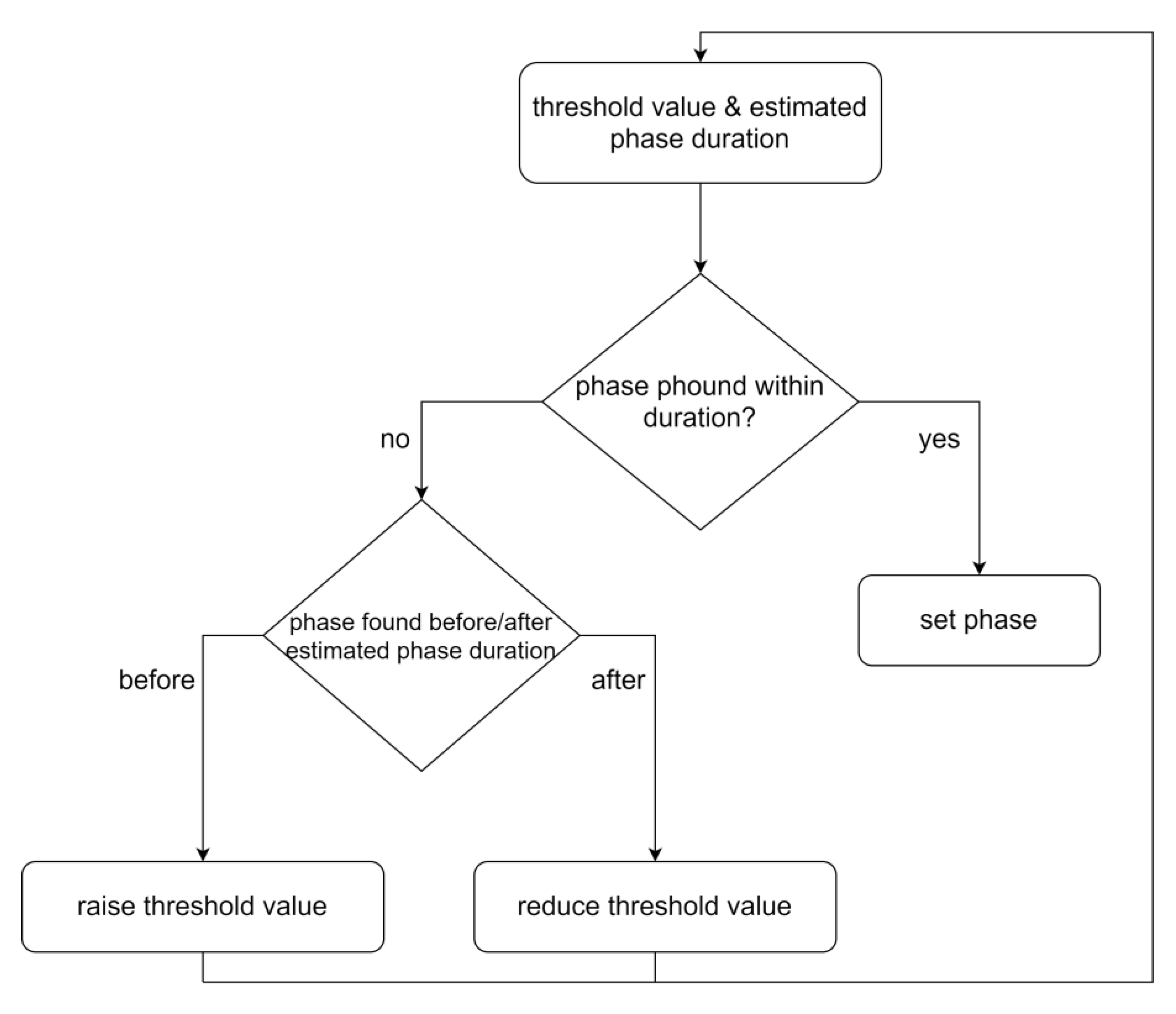
3.3. Step 3: Dynamic Phase Setting
3.3.1. General
3.3.2. Step Signal Phase Settings Algorithms
3.3.3. Intertwined Phase Settings Algorithms
3.4. Step 4: Feature Extraction
3.5. Step 5: Multivariate Analysis
4. Discussion
4.1. Phase Setting
4.2. Outlier Detection
5. Conclusions
Supplementary Materials
Author Contributions
Funding
Acknowledgments
Conflicts of Interest
References
- U.S. Department of Health and Human Services. Process Validation: General Principles and Practices; U.S. Department of Health and Human Services: Washington, DC, USA, 2011.
- Nelson, L.S. The shewhart control chart—Tests for special causes. J. Qual. Technol. 1984, 16, 237–239. [Google Scholar] [CrossRef]
- Boyer, M.; Gampfer, J.; Zamamiri, A.; Payne, R. A roadmap for the implementation of continued process verification. PDA J. Pharm. Sci. Technol. 2016, 70, 282–292. [Google Scholar] [CrossRef]
- BPOG. Continued Process Verification: An Industry Position Paper with Example Plan; Biophorum Operations Group. Available online: https://docplayer.net/21494332-Continued-process-verification-an-industry-position-paper-with-example-plan.html (accessed on 3 June 2020).
- Patro, S.Y.; Freund, E.; Chang, B.S. Protein formulation and fill-finish operations. In Biotechnology Annual Review; Elsevier: Amsterdam, The Netherlands, 2002; Volume 8, pp. 55–84. ISBN 978-0-444-51025-9. [Google Scholar]
- Rathore, N.; Rajan, R.S. Current perspectives on stability of protein drug products during formulation, fill and finish operations. Biotechnol. Prog. 2008, 24, 504–514. [Google Scholar] [CrossRef]
- Montgomery, D.C. Statistical Quality Control, 7th ed.; Wiley: Hoboken, NJ, USA, 1991. [Google Scholar]
- Montgomery, D.C.; Jennings, C.L.; Kulahci, M. Introduction to Time Series Analysis and Forecasting, 2nd ed.; Wiley: Hoboken, NJ, USA, 1976; ISBN 978-1-118-74511-3. [Google Scholar]
- Geurts, P. Pattern extraction for time series classification. In Principles of Data Mining and Knowledge Discovery; De Raedt, L., Siebes, A., Eds.; Springer: Berlin/Heidelberg, Germany, 2001; Volume 2168, pp. 115–127. ISBN 978-3-540-42534-2. [Google Scholar]
- Stephanopoulos, G.; Locher, G.; Duff, M.J.; Kamimura, R.; Stephanopoulos, G. Fermentation database mining by pattern recognition. Biotechnol. Bioeng. 1997, 53, 443–452. [Google Scholar] [CrossRef]
- Golabgir, A.; Gutierrez, J.M.; Hefzi, H.; Li, S.; Palsson, B.O.; Herwig, C.; Lewis, N.E. Quantitative feature extraction from the Chinese hamster ovary bioprocess bibliome using a novel meta-analysis workflow. Biotechnol. Adv. 2016, 34, 621–633. [Google Scholar] [CrossRef] [Green Version]
- Chiang, L.H.; Leardi, R.; Pell, R.J.; Seasholtz, M.B. Industrial experiences with multivariate statistical analysis of batch process data. Chemom. Intell. Lab. Syst. 2006, 81, 109–119. [Google Scholar] [CrossRef]
- Vo, A.Q.; He, H.; Zhang, J.; Martin, S.; Chen, R.; Repka, M.A. Application of FT-NIR analysis for in-line and real-time monitoring of pharmaceutical hot melt extrusion: A technical note. AAPS PharmSciTech 2018, 19, 3425–3429. [Google Scholar] [CrossRef]
- Chen, J.; Liu, K.-C. On-line batch process monitoring using dynamic PCA and dynamic PLS models. Chem. Eng. Sci. 2002, 57, 63–75. [Google Scholar] [CrossRef]
- Borchert, D.; Suarez-Zuluaga, D.A.; Sagmeister, P.; Thomassen, Y.E.; Herwig, C. Comparison of data science workflows for root cause analysis of bioprocesses. Bioprocess Biosyst. Eng. 2019, 42, 245–256. [Google Scholar] [CrossRef] [Green Version]
- Donoho, D.L. High-dimensional data analysis: The curses and blessings of dimensionality. AMS Math Chall. Lect. 2000, 1, 1–32. Available online: https://www.researchgate.net/publication/220049061_High-Dimensional_Data_Analysis_The_Curses_and_Blessings_of_Dimensionality (accessed on 2 June 2020).
- Friedman, J.; Hastie, T.; Tibshirani, R. High-dimensional problems: P >> N. In The Elements of Statistical Learning; Springer: Berlin, Germany, 2017; Volume 2, pp. 649–699. [Google Scholar]
- Suarez-Zuluaga, D.A.; Borchert, D.; Driessen, N.N.; Bakker, W.A.M.; Thomassen, Y.E. Accelerating bioprocess development by analysis of all available data: A USP case study. Vaccine 2019, 37, 7081–7089. [Google Scholar] [CrossRef]
- Steinwandter, V.; Borchert, D.; Herwig, C. Data science tools and applications on the way to Pharma 4.0. Drug Discov. Today 2019. [Google Scholar] [CrossRef]
- Hubert, M.; Rousseeuw, P.J.; Vanden Branden, K. ROBPCA: A new approach to robust principal component analysis. Technometrics 2005, 47, 64–79. [Google Scholar] [CrossRef]
- Hotelling, H. Analysis of a complex of statistical variables into principal components. J. Educ. Psychol. 1933, 24, 417–441. [Google Scholar] [CrossRef]
- Zhu, X.; Wu, X. Class noise vs. attribute noise: A quantitative study. Artif. Intell. Rev. 2004, 22, 177–210. [Google Scholar] [CrossRef]
- Brownrigg, D.R.K. The weighted median filter. Commun. ACM 1984, 27, 807–818. [Google Scholar] [CrossRef]
- Lee, J.-M.; Yoo, C.K.; Lee, I.-B. Enhanced process monitoring of fed-batch penicillin cultivation using time-varying and multivariate statistical analysis. J. Biotechnol. 2004, 110, 119–136. [Google Scholar] [CrossRef]
- Agrawal, R.; Nyamful, C. Challenges of big data storage and management. Glob. J. Inf. Technol. 2016, 6. [Google Scholar] [CrossRef]
- De Maesschalck, R.; Jouan-Rimbaud, D.; Massart, D.L. The mahalanobis distance. Chemom. Intell. Lab. Syst. 2000, 50, 1–18. [Google Scholar] [CrossRef]
- Brereton, R.G. The Mahalanobis distance and its relationship to principal component scores: The Mahalanobis distance and PCA. J. Chemom. 2015, 29, 143–145. [Google Scholar] [CrossRef]
- Charaniya, S.; Hu, W.-S.; Karypis, G. Mining bioprocess data: Opportunities and challenges. Trends Biotechnol. 2008, 26, 690–699. [Google Scholar] [CrossRef] [PubMed]
- Ho, T.K. Random decision forests. In Proceedings of the 3rd International Conference on Document Analysis and Recognition, Montreal, QC, Canada, 14–16 August 1995; pp. 278–282. [Google Scholar]
- Batista, G.E.A.P.A.; Prati, R.C.; Monard, M.C. A study of the behavior of several methods for balancing machine learning training data. ACM SIGKDD Explor. Newsl. 2004, 6, 20. [Google Scholar] [CrossRef]
- Todorov, V.; Templ, M.; Filzmoser, P. Detection of multivariate outliers in business survey data with incomplete information. Adv. Data Anal. Classif. 2011, 5, 37–56. [Google Scholar] [CrossRef] [Green Version]
- Filzmoser, P. A Multivariate Outlier Detection Method. 2004. Available online: http://file.statistik.tuwien.ac.at/filz/papers/minsk04.pdf (accessed on 2 June 2020).


| Quality Data | Sterile Filtration | Lyophilization | ||||||
|---|---|---|---|---|---|---|---|---|
| Data Type | Feature | Time-series | Time-series | |||||
| Description | Abbr. | Description | Abbr. | Unit | Description | Abbr. | Unit | |
| Monitored Output | CQA data of bulk drug substance (BDS) | CQA data | Temperature of product | SF1 | (°C) | Inlet temperature | LP1 | (°C) |
| Time stamps of start and end of sterile filtration and lyophilization | Time stamps | Applied pressure | SF2 | (bar) | Outlet temperature | LP2 | (°C) | |
| Weight of unfiltered product | SF3 | (kg) | Chamber vacuum 1 | LP3 | (bar) | |||
| Chamber vacuum 2 | LP4 | (bar) | ||||||
| Temperature of liquid nitrogen | LP5 | (°C) | ||||||
| Condenser pressure | LP6 | (bar) | ||||||
| Condenser vacuum | LP7 | (bar) | ||||||
| Phase Name | Condition | Run Order |
|---|---|---|
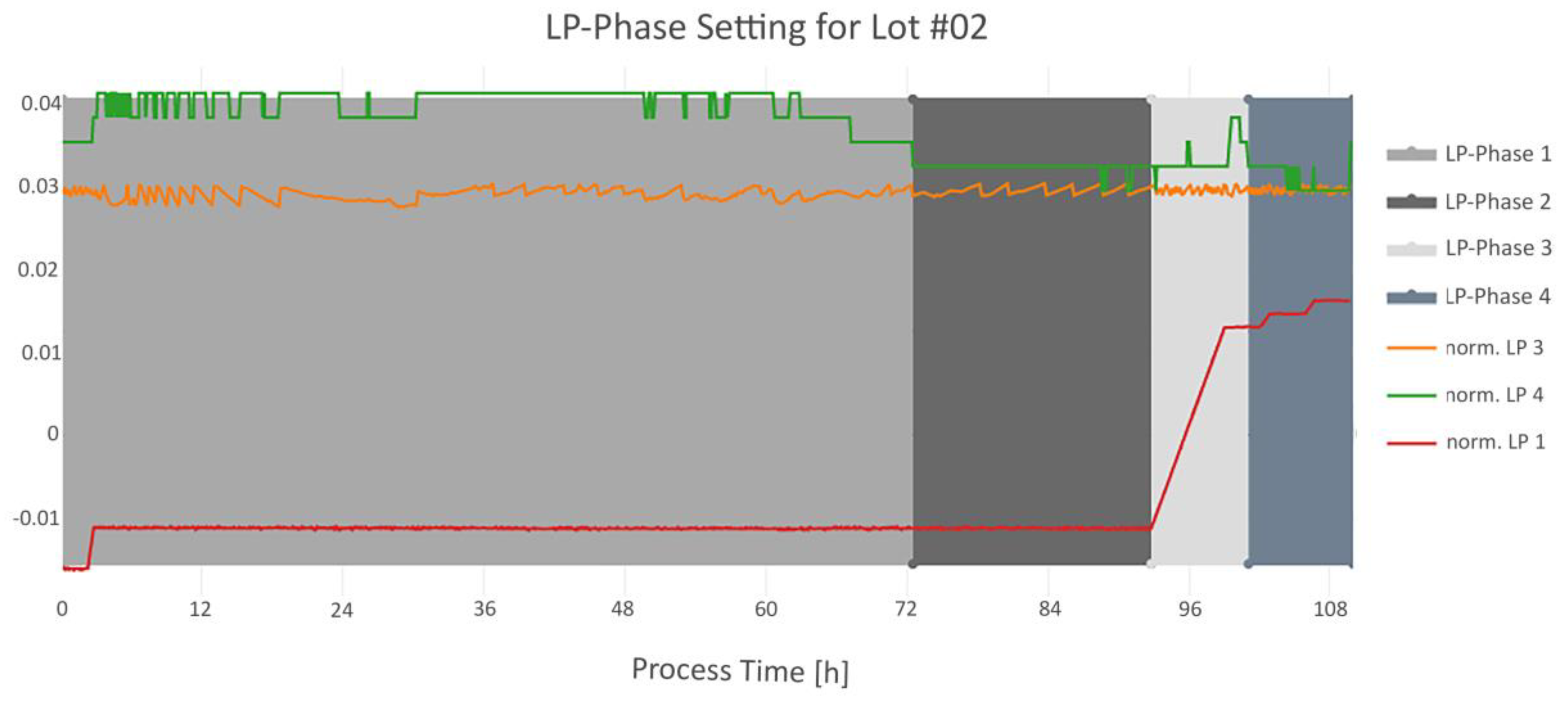
| LP-Phase 1 | Starts with the beginning of LP4 signal. Ends with the start of LP-Phase 2. | 2 |
| LP-Phase 2 | First timestamp, where the difference between LP3 and LP4 is below 20%. Ends with the increasing slope of LP1. | 1 |
| LP-Phase 3 | Starts with the end of LP-Phase 2. Ends when LP4 has the same value as at the beginning of LP-Phase 2, within certain time range. | 3 |
| LP-Phase 4 | Starts with the end of LP-Phase 3. Ends with end of LP4. | 4 |
| Score Distance | Orthogonal Distance | |||
|---|---|---|---|---|
| Moderate Outlier | Outlier | Moderate Outlier | Outlier | |
| CPCA | 6 | 4 | - | 9 |
| ROBPCA | 7 | 1 | 1 | 0 |
© 2020 by the authors. Licensee MDPI, Basel, Switzerland. This article is an open access article distributed under the terms and conditions of the Creative Commons Attribution (CC BY) license (http://creativecommons.org/licenses/by/4.0/).
Share and Cite
Pretzner, B.; Taylor, C.; Dorozinski, F.; Dekner, M.; Liebminger, A.; Herwig, C. Multivariate Monitoring Workflow for Formulation, Fill and Finish Processes. Bioengineering 2020, 7, 50. https://0-doi-org.brum.beds.ac.uk/10.3390/bioengineering7020050
Pretzner B, Taylor C, Dorozinski F, Dekner M, Liebminger A, Herwig C. Multivariate Monitoring Workflow for Formulation, Fill and Finish Processes. Bioengineering. 2020; 7(2):50. https://0-doi-org.brum.beds.ac.uk/10.3390/bioengineering7020050
Chicago/Turabian StylePretzner, Barbara, Christopher Taylor, Filip Dorozinski, Michael Dekner, Andreas Liebminger, and Christoph Herwig. 2020. "Multivariate Monitoring Workflow for Formulation, Fill and Finish Processes" Bioengineering 7, no. 2: 50. https://0-doi-org.brum.beds.ac.uk/10.3390/bioengineering7020050