Spectral Decomposition and Sound Source Localization of Highly Disturbed Flow through a Severe Arterial Stenosis

 ,
, 
 ,
, 
Abstract
:1. Introduction
2. Materials and Methods
2.1. Computational Model
2.2. Physics and Flow Conditions
2.3. Proper Orthogonal Decomposition (POD) Analysis
2.4. Mesh
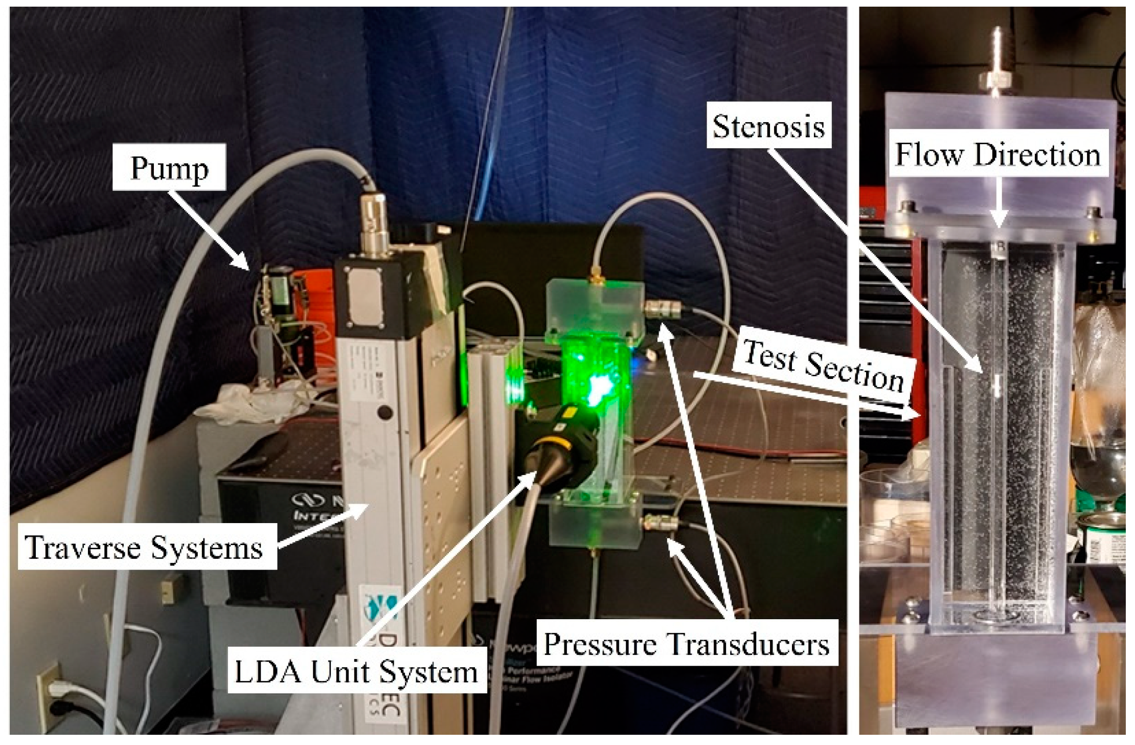
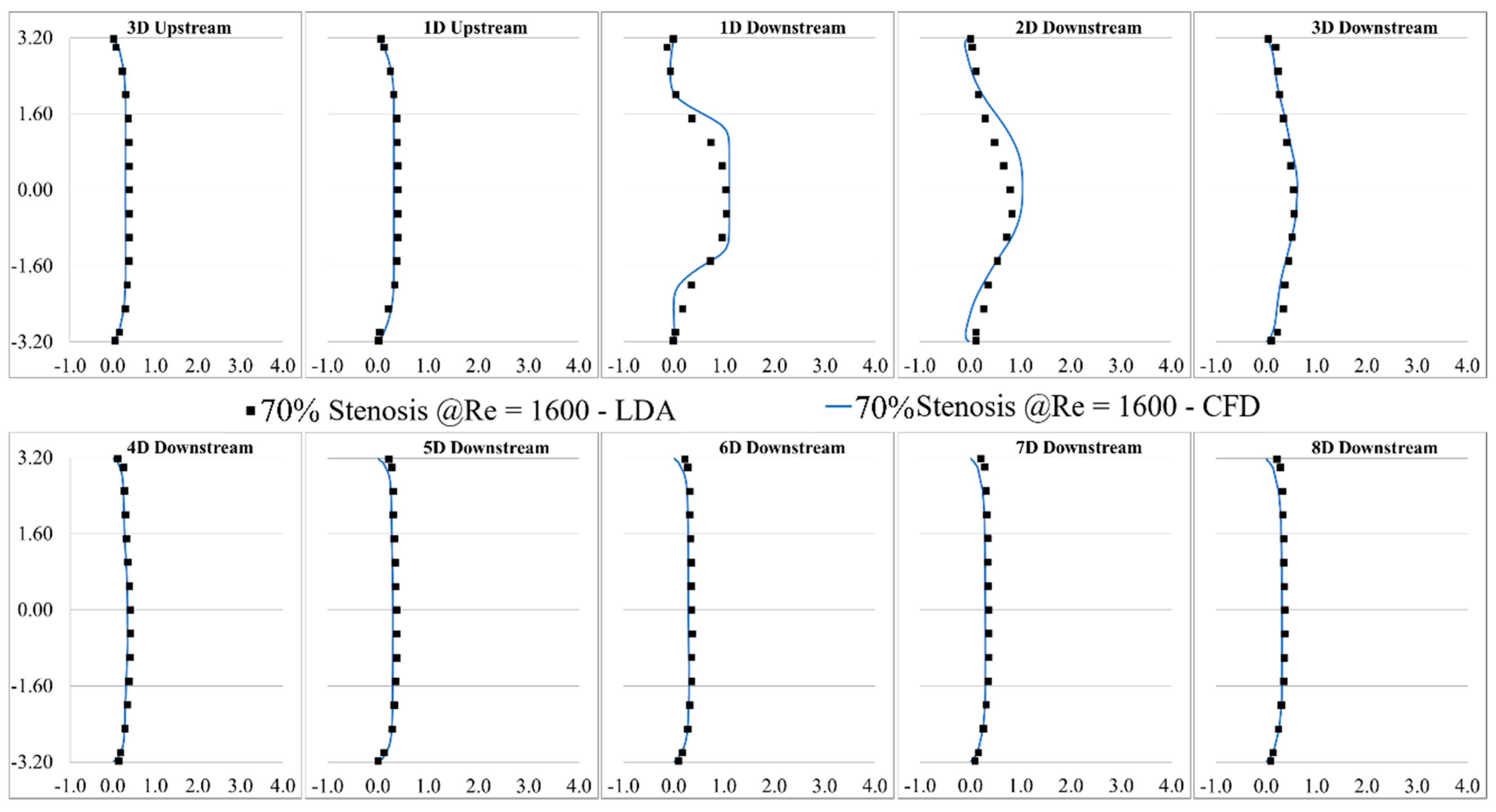
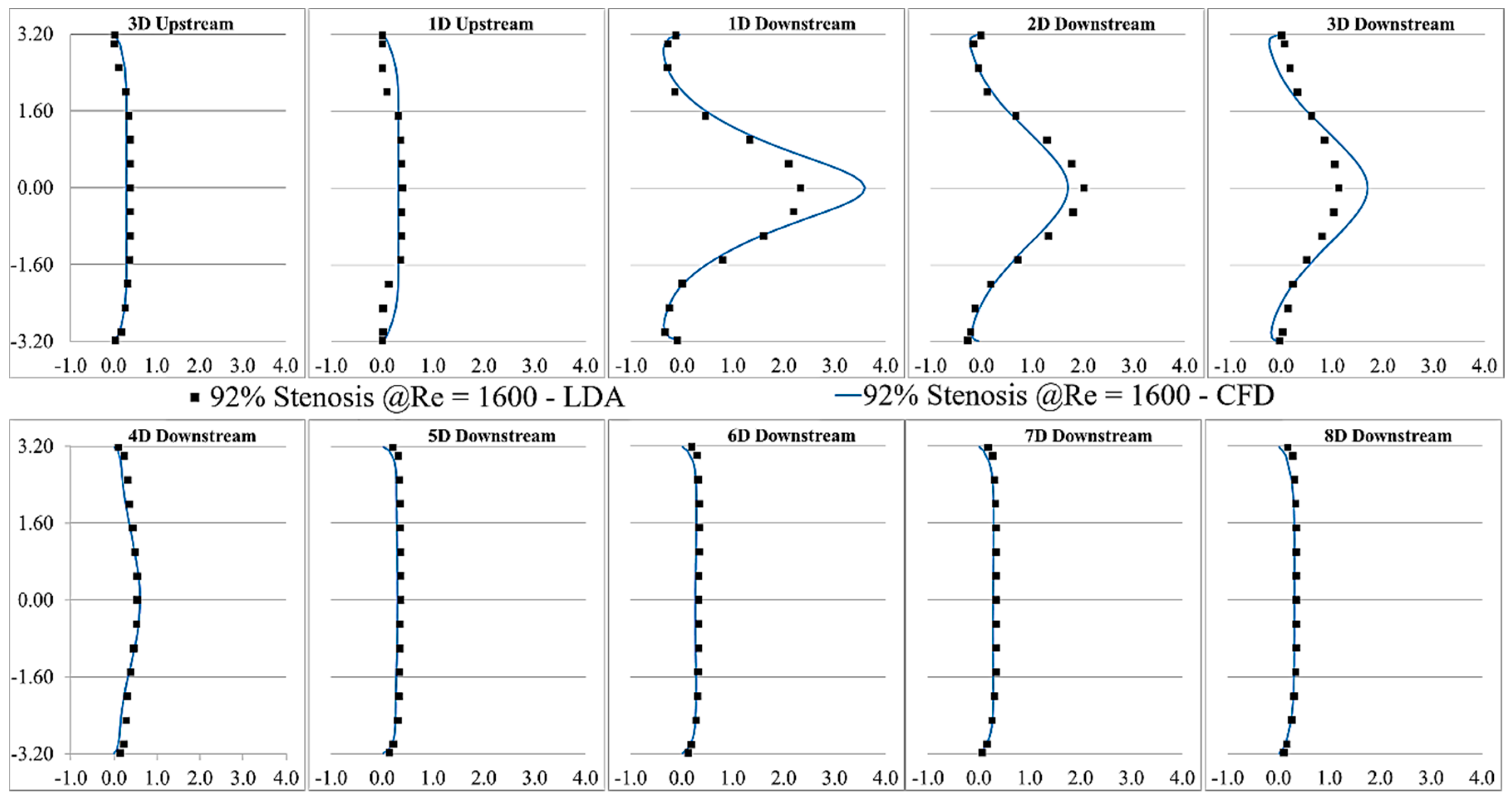
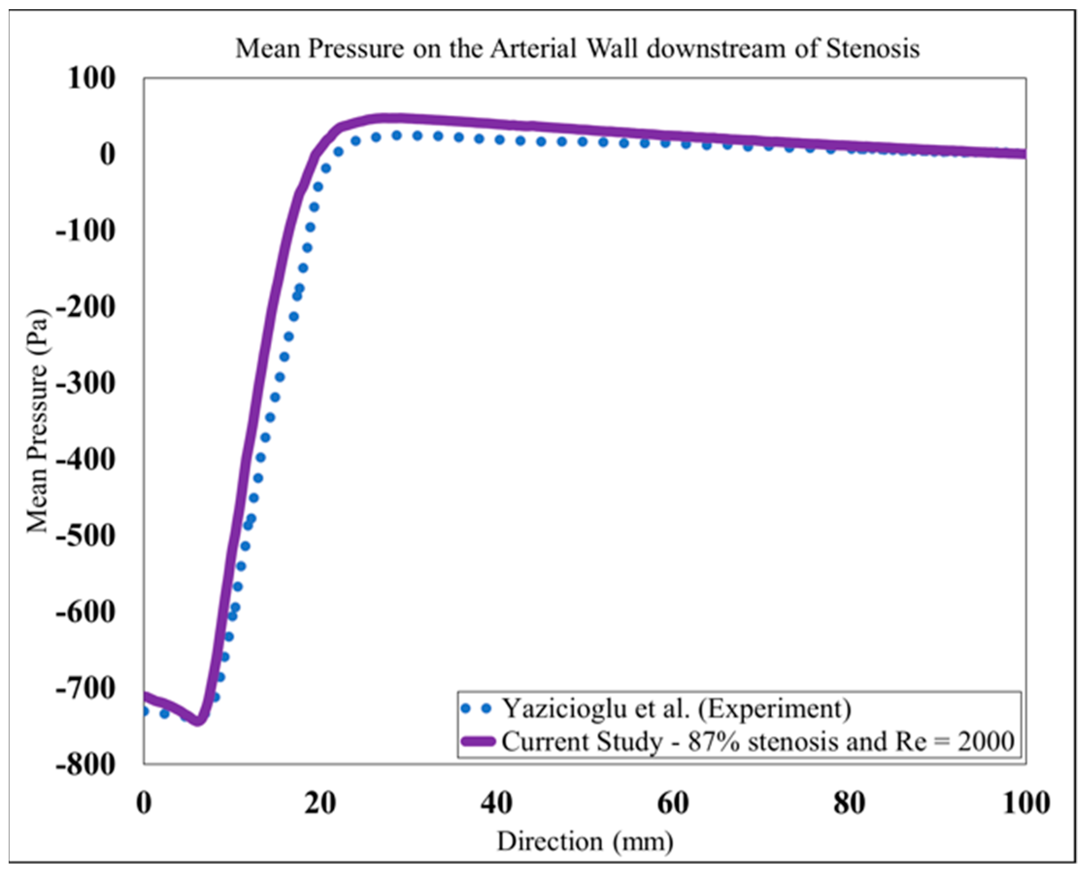
2.5. Validation
3. Results and Discussions
4. Conclusions
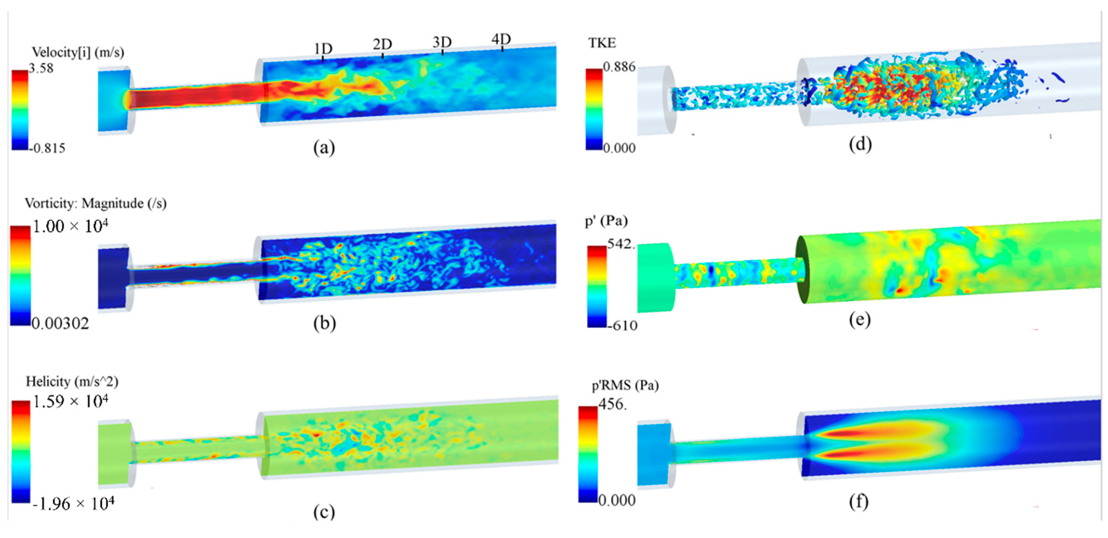
- The analysis of the flow solution showed that the flow velocity increased significantly inside the stenosis and became unstable, leading to significant pressure fluctuations at the plaque surface. It indicates the possibility of increased fluid-solid interactions and subsequent excitation of the vessel wall;
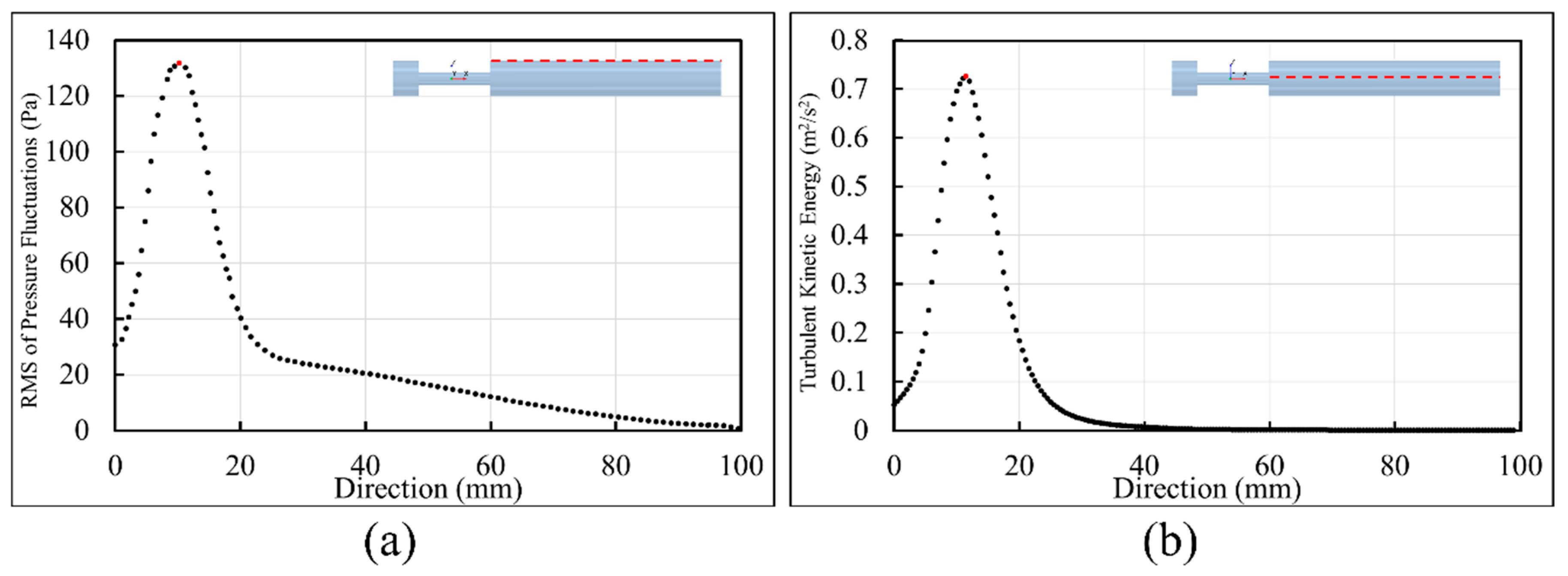
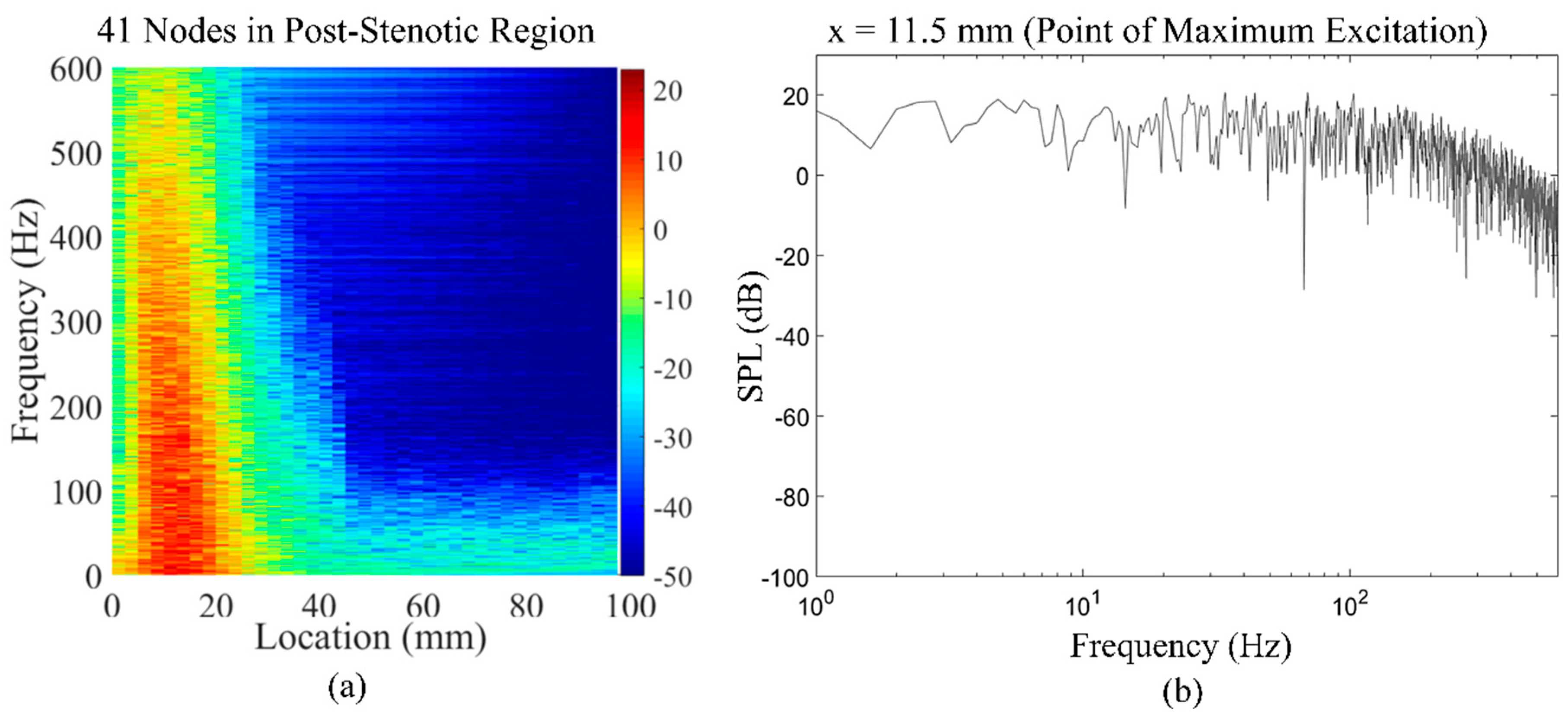
- As the flow jet entered into the expansion region, flow separation occurred at x = 1D, where large eddies started to cascade into smaller eddies with higher rotational energies, up to 4D downstream of the stenosis. These eddies were the origin of flow-induced acoustic radiation, which was mostly concentrated around x = 11.5 mm, as the point of maximum excitation. It is important to avoid this region and move the measurement probe further downstream (i.e., x > 4D) of the vessel during coronary catheterization measurements such as the fractional flow reserve (FFR) for accurate readings;
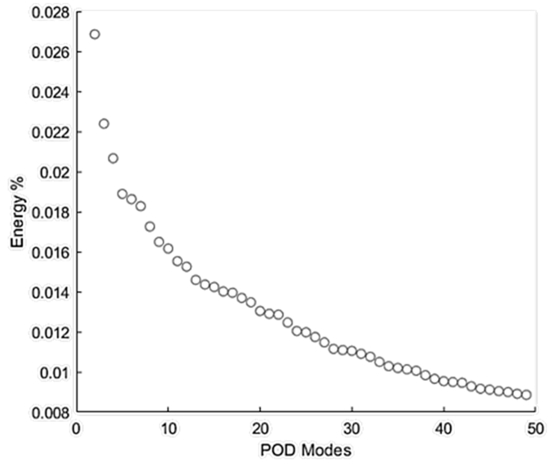
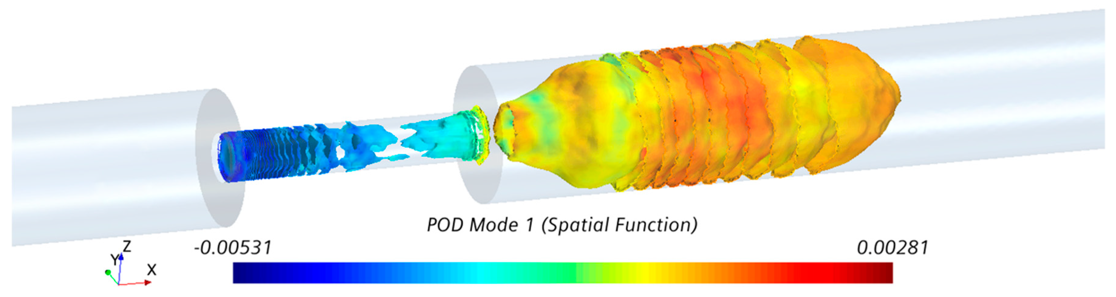
- The analysis of the spectra of the recorded pressures at the wall also showed that the most energetic POD mode of the flow appeared in the same regions, which complimented the results from the fluid dynamics analysis;
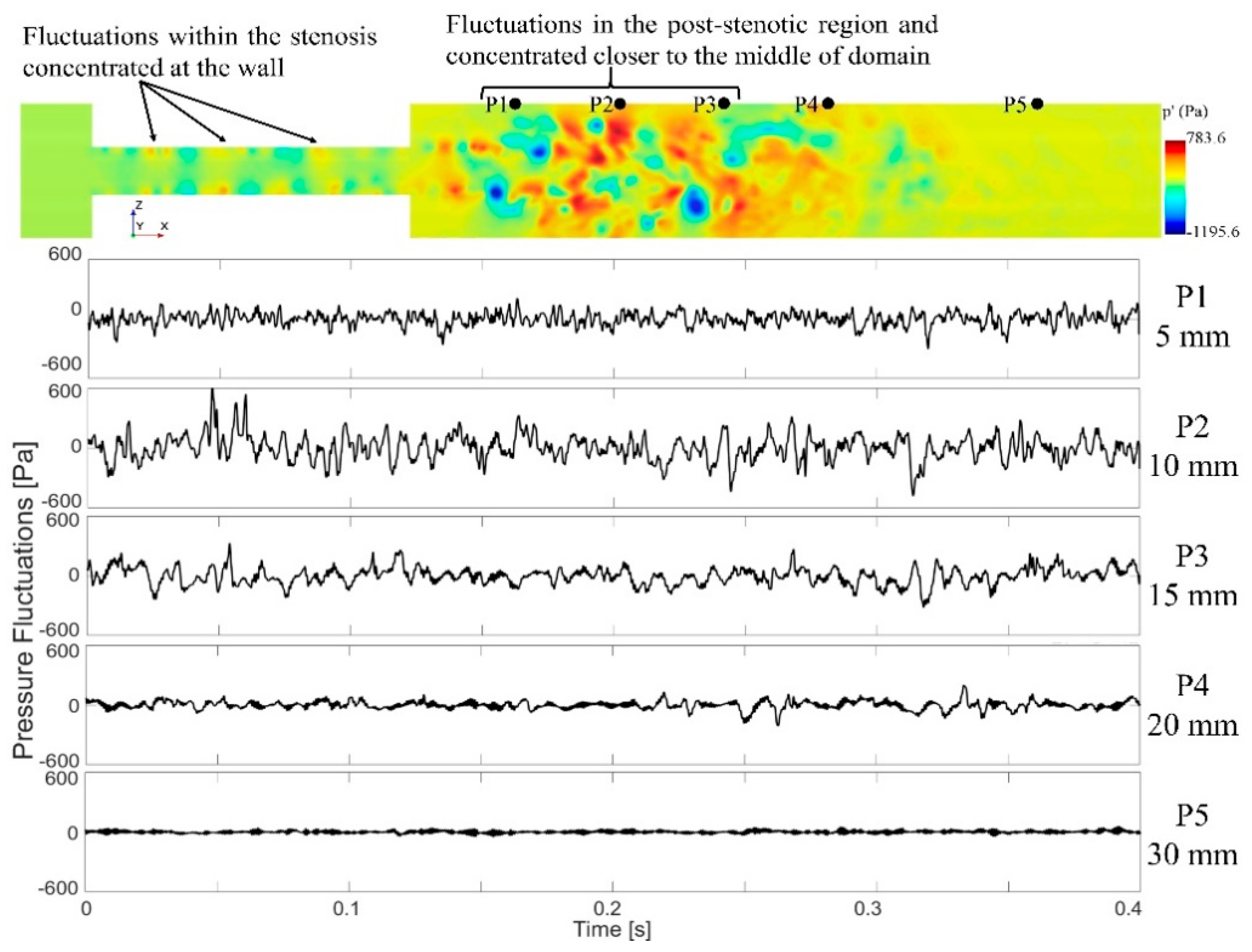
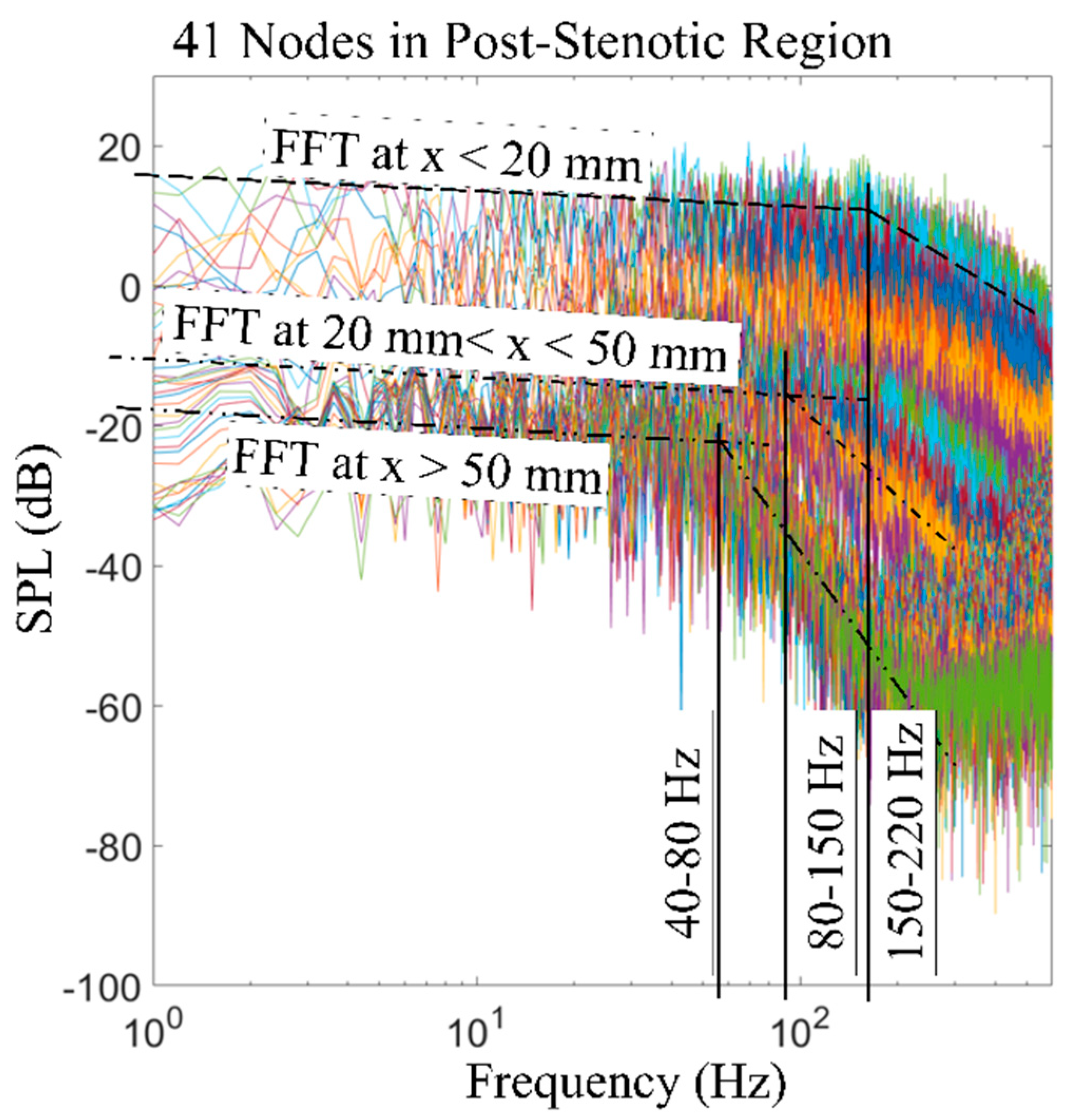
- The spectral decomposition of the pressure fluctuations showed broadband acoustic sources distributed in the same region (1D to 4D) generated from turbulence.
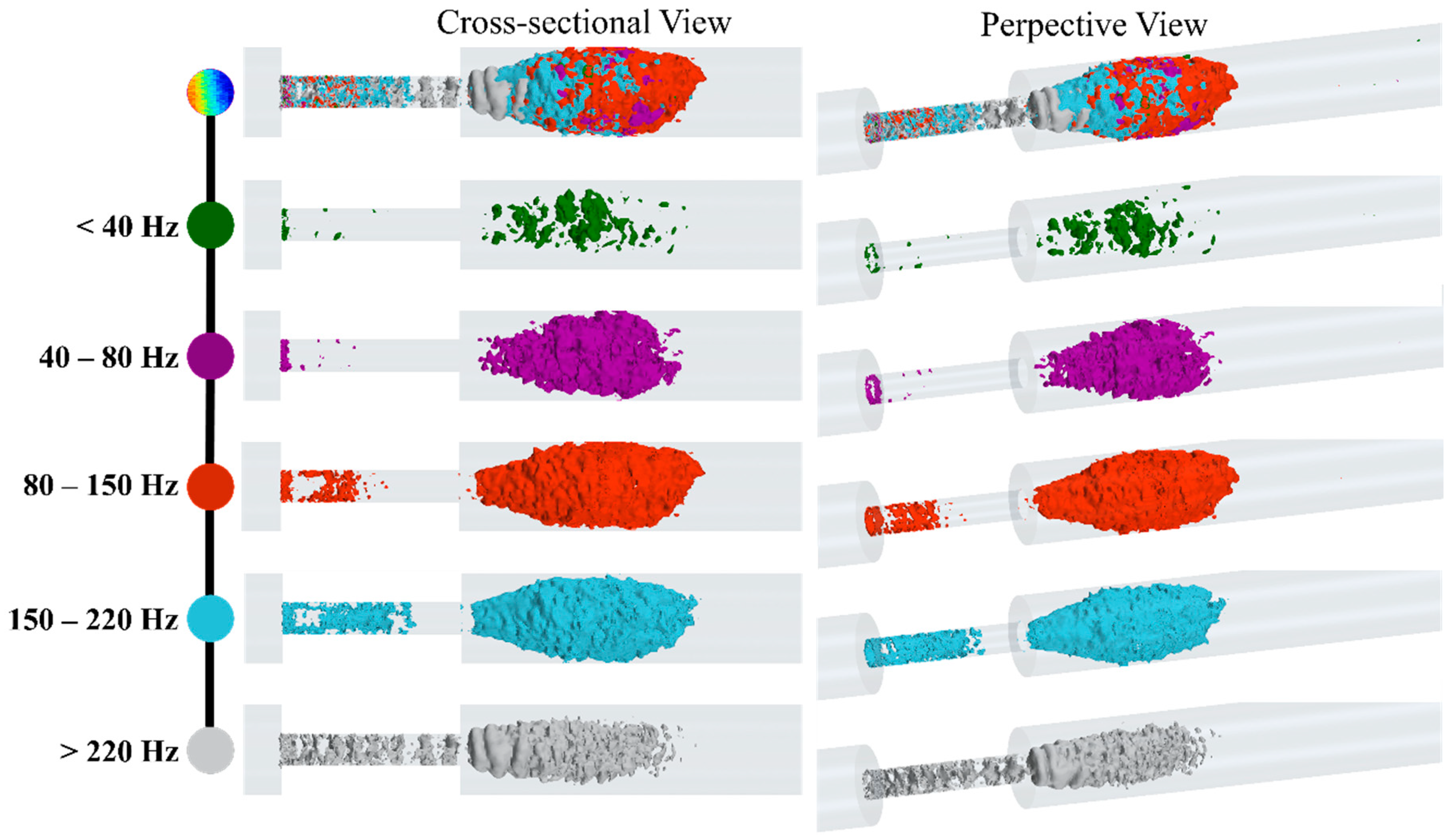
- Low-frequency (i.e., <40 Hz) acoustic fluctuations were observed mostly around the flow jet and the separation regions, which were correlated with larger eddies. The break frequency, as a characteristic of the sound transmitted through the vessel wall and surrounding tissue, was considered in the temporal filtering of the acoustic pressure;
- At higher frequency ranges between 80 Hz to 220 Hz, the fluctuations related to smaller eddies appeared at the entrance of the stenosis and, in the middle of the fluctuating region, extended up to 4D downstream of the stenosis;
- The results also showed organized ring-like isosurfaces of fluctuations inside the stenosis at high frequencies over 220 Hz.
5. Application Feasibility
6. Future Works
- The modeling of flow-induced acoustics in patient-specific models derived from medical imaging. Although the simplified concentric stenosis geometry can help derive qualitative conclusions, the patient-specific irregular stenosis profiles can lead to specific alterations in the generated sounds;
- An acoustic analysis of the progression of stenosis at different levels of severity. The understanding of sound signatures of a stenosis at different stages of the disease can assist to develop an algorithm for the early detection of the stenosis;
- A pulsatile patient-specific flow. The steady flow assumption in this study represented the peak systole of the pulsatile flow. However, the pulsatile flow, with the turbulent diffusion during the diastole with lower flow rates, generates more homogeneous spectra;
- Modeling of elastic wall structural response. Although we verified the use of a rigid wall for this study according to the literature, we should agree that, for the studies focused more on the correlation of hemodynamic parameters with the gradual development of stenosis size and the interactions between the flow and the artery wall, especially with different stiffness of the stenosis, artery, and surrounding tissue, the modeling assumption of an elastic wall becomes more relevant and acceptable.
Author Contributions
Funding
Institutional Review Board Statement
Informed Consent Statement
Data Availability Statement
Acknowledgments
Conflicts of Interest
References
- Centers for Disease Control and Prevention Underlying Cause of Death 1999–2018. CDC WONDER Online Database 2020. U.S. Department of Health & Human Services: Washington, DC, USA. Available online: https://wonder.cdc.gov/ucd-icd10.html (accessed on 25 December 2020).
- Mozaffarian, D.; Benjamin, E.J.; Go, A.S.; Arnett, D.K.; Blaha, M.J.; Cushman, M.; Das, S.R.; de Ferranti, S.; Després, J.-P.; Fullerton, H.J.; et al. Heart Disease and Stroke Statistics—2016 Update: A Report From the American Heart Association. Circulation 2016, 133, e38–e360. [Google Scholar] [CrossRef]
- Rosamond, W.; Flegal, K.; Friday, G.; Furie, K.; Go, A.; Greenlund, K.; Haase, N.; Ho, M.; Howard, V.; Kissela, B.; et al. Heart disease and stroke statistics—2007 Update: A report from the American Heart Association Statistics Committee and Stroke Statistics Subcommittee. Circulation 2007, 115, e69–e171. [Google Scholar] [CrossRef]
- AHA (American Heart Association). Cardiovascular Disease: A Costly Burden, for America Projections Through 2035; American Heart Association Federation Advocacy: Washington, DC, USA, 2017. [Google Scholar]
- Fryar, C.D.; Chen, T.C.; Li, X. Prevalence of uncontrolled risk factors for cardiovascular disease: United States, 1999–2010. NCHS Data Brief 2012, 103, 1–8. [Google Scholar]
- Ahmed, S.A.; Giddens, D.P. Giddens Flow disturbance measurements through a constricted tube at moderate Reynolds numbers. J. Biomech. 1983, 16, 955–963. [Google Scholar] [CrossRef]
- Kirkeeide, R.L.; Young, D.F.; Cholvin, N. Cholvin Wall vibrations induced by flow through simulated stenoses in models and arteries. J. Biomech. 1977, 10, 431–441. [Google Scholar] [CrossRef]
- Khalili, F.; Gamage, P.P.T.; A Mansy, H. Verification of Turbulence Models for Flow in a Constricted Pipe at Low Reynolds Number. In Proceedings of the 3rd Thermal and Fluids Engineering Conference (TFEC), Fort Lauderdale, FL, USA, 4–7 March 2018; pp. 1–10. [Google Scholar]
- Ahmed, S.A. An experimental investigation of pulsatile flow through a smooth constriction. Exp. Therm. Fluid Sci. 1998, 17, 309–318. [Google Scholar] [CrossRef]
- Salim, S.M.; Ariff, M.; Cheah, S.C. Wall Y + Approach for Dealing With Turbulent Flow Over a Surface Mounted Cube: Part 1—Low Reynolds Number. Prog. Comput. Fluid Dyn. Int. J. 2010, 10, 341. [Google Scholar] [CrossRef]
- Fredberg, J.J. Origin and character of vascular murmurs: Model studies. J. Acoust. Soc. Am. 1977, 61, 1077–1085. [Google Scholar] [CrossRef]
- Seo, J.H.; Bakhshaee, H.; Garreau, G.; Zhu, C.; Andreou, A.; Thompson, W.R.; Mittal, R. A method for the computational modeling of the physics of heart murmurs. J. Comput. Phys. 2017, 336, 546–568. [Google Scholar] [CrossRef] [Green Version]
- Bruns, D.L. A general theory of the causes of murmurs in the cardiovascular system. Am. J. Med. 1959, 27, 360–374. [Google Scholar] [CrossRef]
- Lees, R.S.; Dewey, C.F. Phonoangiography: A new noninvasive diagnostic method for studying arterial disease. Proc. Natl. Acad. Sci. USA 1970, 67, 935–942. [Google Scholar] [CrossRef] [PubMed] [Green Version]
- Lee, S.E.; Lee, S.W.; Fischer, P.F.; Bassiouny, H.S.; Loth, F. Direct numerical simulation of transitional flow in a stenosed carotid bifurcation. J. Biomech. 2008, 41, 2551–2561. [Google Scholar] [CrossRef] [Green Version]
- Mittal, R.C.; Simmons, S.P.; Najjar, F.M. Numerical study of pulsatile flow in a constricted channel. J. Fluid Mech. 2003, 485, 337–378. [Google Scholar] [CrossRef] [Green Version]
- Seo, J.H.; Mittal, R. A coupled flow-acoustic computational study of bruits from a modeled stenosed artery. Med. Biol. Eng. Comput. 2012, 50, 1025–1035. [Google Scholar] [CrossRef] [PubMed]
- Khalili, F.; Gamage, P.P.T.; Meguid, I.A.; Mansy, H.A. A coupled CFD-FEA study of sound generated in a stenosed artery and transmitted through tissue layers. In Proceedings of the SoutheastCon 2018, St. Petersburg, FL, USA, 19–22 April 2018. [Google Scholar] [CrossRef]
- Salman, H.E.; Yazicioglu, Y. Flow-induced vibration analysis of constricted artery models with surrounding soft tissue. J. Acoust. Soc. Am. 2017, 142, 1913–1925. [Google Scholar] [CrossRef] [PubMed]
- Salman, H.E.; Yazicioglu, Y. Experimental and numerical investigation on soft tissue dynamic response due to turbulence-induced arterial vibration. Med. Biol. Eng. Comput. 2019, 57, 1737–1752. [Google Scholar] [CrossRef]
- Thomas, J.L.; Winther, S.; Wilson, R.F.; Bøttcher, M. A novel approach to diagnosing coronary artery disease: Acoustic detection of coronary turbulence. Int. J. Cardiovasc. Imaging 2017, 33, 129–136. [Google Scholar] [CrossRef]
- Makaryus, A.N.; Makaryus, J.N.; Figgatt, A.; Mulholland, D.; Kushner, H.; Semmlow, J.L.; Mieres, J.; Taylor, A.J. Utility of an advanced digital electronic stethoscope in the diagnosis of coronary artery disease compared with coronary computed tomographic angiography. Am. J. Cardiol. 2013, 111, 786–792. [Google Scholar] [CrossRef] [PubMed]
- Winther, S.; Schmidt, S.E.; Holm, N.R.; Toft, E.; Struijk, J.J.; Bøtker, H.E.; Bøttcher, M. Diagnosing coronary artery disease by sound analysis from coronary stenosis induced turbulent blood flow: Diagnostic performance in patients with stable angina pectoris. Int. J. Cardiovasc. Imaging 2016, 32, 235–245. [Google Scholar] [CrossRef] [PubMed] [Green Version]
- Tobin, R.J.; Chang, I.D. Wall pressure spectra scaling downstream of stenoses in steady tube flow. J. Biomech. 1976, 9, 633–640. [Google Scholar] [CrossRef]
- Beach, T.G.; Maarouf, C.L.; Brooks, R.G.; Shirohi, S.; Daugs, I.D.; Sue, L.I.; Sabbagh, M.N.; Walker, D.G.; Lue, L.; Roher, A.E. Reduced clinical and postmortem measures of cardiac pathology in subjects with advanced Alzheimer’s disease. BMC Geriatr. 2011, 11, 3. [Google Scholar] [CrossRef] [PubMed] [Green Version]
- Yazicioglu, Y.; Royston, T.J.; Spohnholtz, T.; Martin, B.; Loth, F.; Bassiouny, H.S. Acoustic radiation from a fluid-filled, subsurface vascular tube with internal turbulent flow due to a constriction. J. Acoust. Soc. Am. 2005, 118, 1193–1209. [Google Scholar] [CrossRef] [PubMed]
- Sandgren, T.; Sonesson, B.; Ahlgren, A.R.; Lanne, T. The diameter of the common femoral artery in healthy human: Influence of sex, age, and body size. J. Vasc. Surg. 1999, 29, 503–510. [Google Scholar] [CrossRef] [Green Version]
- Chami, H.A.; Keyes, M.J.; Vita, J.A.; Mitchell, G.F.; Larson, M.G.; Fan, S.; Vasan, R.S.; O’Connor, G.T.; Benjamin, E.J.; Gottlieb, D.J. Brachial artery diameter, blood flow and flow-mediated dilation in sleep-disordered breathing. Vasc. Med. 2009, 14, 351–360. [Google Scholar] [CrossRef]
- Salman, H.E.; Sert, C.; Yazicioglu, Y. Computational analysis of high frequency fluid-structure interactions in constricted flow. Comput. Struct. 2013, 122, 145–154. [Google Scholar] [CrossRef]
- Borisyuk, A.O. Experimental study of wall pressure fluctuations in rigid and elastic pipes behind an axisymmetric narrowing. J. Fluids Struct. 2010, 26, 658–674. [Google Scholar] [CrossRef]
- Mamun, K.; Rahman, M.M.; Akhter, M.N.; Ali, M. Physiological non-Newtonian blood flow through single stenosed artery. AIP Conf. Proc. 2016, 1754, 040001. [Google Scholar] [CrossRef]
- Jabir, E.; Lal, S.A. Numerical analysis of blood flow through an elliptic stenosis using large eddy simulation. Proc. Inst. Mech. Eng. Part H J. Eng. Med. 2016, 230, 709–726. [Google Scholar] [CrossRef] [PubMed]
- Mancini, V.; Bergersen, A.W.; Vierendeels, J.; Segers, P.; Valen-Sendstad, K. High-Frequency Fluctuations in Post-stenotic Patient Specific Carotid Stenosis Fluid Dynamics: A Computational Fluid Dynamics Strategy Study. Cardiovasc. Eng. Technol. 2019, 10, 277–298. [Google Scholar] [CrossRef] [Green Version]
- Valen-Sendstad, K.; Steinman, D.A. Mind the gap: Impact of computational fluid dynamics solution strategy on prediction of intracranial aneurysm hemodynamics and rupture status indicators. Am. J. Neuroradiol. 2014, 35, 536–543. [Google Scholar] [CrossRef] [Green Version]
- Raschi, M.; Mut, F.; Byrne, G.; Putman, C.M.; Tateshima, S.; Viñuela, F.; Tanoue, T.; Tanishita, K.; Cebral, J.R. CFD and PIV analysis of hemodynamics in a growing intracranialaneurysm. Int. J. Numer. Methods Biomed. Eng. 2012, 28, 214–228. [Google Scholar] [CrossRef] [Green Version]
- Ozden, K.; Sert, C.; Yazicioglu, Y. Numerical investigation of wall pressure fluctuations downstream of concentric and eccentric blunt stenosis models. Proc. Inst. Mech. Eng. Part H J. Eng. Med. 2020, 234, 48–60. [Google Scholar] [CrossRef]
- Gayathri, K.; Shailendhra, K. Pulsatile blood flow in large arteries: Comparative study of Burton’s and McDonald’s models. Appl. Math. Mech. 2014, 35, 575–590. [Google Scholar] [CrossRef]
- Cassanova, R.; Giddens, D. Disorder distal to modeled stenoses in steady and pulsatile flow. J. Biomech. 1978, 11, 441–453. [Google Scholar] [CrossRef]
- Tan, F.P.P.; Wood, N.B.; Tabor, G.; Xu, X.Y. Comparison of les of steady transitional flow in an idealized stenosed axisymmetric artery model with a RANS transitional model. J. Biomech. Eng. 2011, 133, 051001. [Google Scholar] [CrossRef] [PubMed]
- Paul, M.; Molla, M. Investigation of physiological pulsatile flow in a model arterial stenosis using large-eddy and direct numerical simulations. Appl. Math. Model. 2012, 36, 4393–4413. [Google Scholar] [CrossRef]
- Rhie, C.M.; Chow, W.L. CHOW Numerical study of the turbulent flow past an airfoil with trailing edge separation. AIAA J. 1983, 21, 1525–1532. [Google Scholar] [CrossRef]
- Violato, D.; Scarano, F. Three-dimensional vortex analysis and aeroacoustic source characterization of jet core breakdown. Phys. Fluids 2013, 25, 015112. [Google Scholar] [CrossRef] [Green Version]
- Freund, J.B.; Colonius, T. Turbulence and Sound-Field POD Analysis of a Turbulent Jet. Int. J. Aeroacoustics 2009, 8, 337–354. [Google Scholar] [CrossRef]
- Mansy, H.A.; Gamage, P.T.; Khalili, F. Aero--acoustics in constricted pipe flow at low mach number. J. Appl. Biotechnol. Bioeng. 2018, 5, 306–309. [Google Scholar] [CrossRef]
- Salim, S.M.; Cheah, S.C. Wall y + Strategy for Dealing with Wall-bounded Turbulent Flows. In Proceedings of the International MultiConference of Engineers and Computer Scientists, Hong Kong, China, 18–20 March 2009; Volume II, pp. 1–6. [Google Scholar]
- Celik, I.; Klein, M.; Janicka, J. Assessment measures for engineering LES applications. J. Fluids Eng. Trans. ASME 2009, 131, 031102. [Google Scholar] [CrossRef]
- Back, L.H.; Roschke, E.J. Shear-layer flow regimes and wave instabilities and reattachment lengths downstream of an abrupt circular channel expansion. J. Appl. Mech. Trans. ASME 1972, 39, 677–681. [Google Scholar] [CrossRef]
- Gamage, P.P.T.; Khalili, F.; Mansy, H.A. Numerical Modeling of Pulse Wave Propagation in a Stenosed Artery using Two-Way Coupled Fluid Structure Interaction (FSI). In Proceedings of the 3rd Thermal and Fluids Engineering Conference (TFEC), Fort Lauderdale, FL, USA, 4–7 March 2018. [Google Scholar]
- Gamage, P.T. Modeling of flow generated sound in a constricted duct at low Mach number flow. Fluid Dyn. 2017. [Google Scholar] [CrossRef]
- Borisyuk, A.O. Model study of noise field in the human chest due to turbulent flow in a larger blood vessel. J. Fluids Struct. 2003, 17, 1095–1110. [Google Scholar] [CrossRef]
- Borisyuk, A.O. Modeling of noise generation by a vascular stenosis. Int. J. Fluid Mech. Res. 2002, 29, 24. [Google Scholar] [CrossRef]
- PLu, C.; Gross, D.R.; Hwang, N.H.C. Intravascular pressure and velocity fluctuations in pulmonic arterial stenosis. J. Biomech. 1980, 13, 291–300. [Google Scholar] [CrossRef]
- Bombardini, T.; Gemignani, V.; Bianchini, E.; Venneri, L.; Petersen, C.; Pasanisi, E.; Pratali, L.; Pianelli, M.; Faita, F.; Giannoni, M.; et al. Cardiac reflections and natural vibrations: Force-frequency relation recording system in the stress echo lab. Cardiovasc. Ultrasound 2007, 5, 42. [Google Scholar] [CrossRef] [PubMed] [Green Version]
- Owsley, N.L. Beamformed nearfield imaging of a simulated coronary artery containing a stenosis. IEEE Trans. Med. Imaging 1998, 17, 900–909. [Google Scholar] [CrossRef] [PubMed] [Green Version]
- Chassaing, C.E.; Stearns, S.D.; van Horn, M.H.; Ryden, C.A. Non-Invasive Turbulent Blood Flow Imaging System. U.S. Patent 6278890B1, 21 August 2001. [Google Scholar]
- Gamage, P.T.; Azad, M.K.; Taebi, A.; Sandler, R.H.; Mansy, H.A. Clustering of SCG Events Using Unsupervised Machine Learning. In Signal Processing in Medicine and Biology; Springer: Berlin/Heidelberg, Germany, 2020; pp. 205–233. [Google Scholar]
- Fillinger, M.F.; Reinitz, E.R.; Schwartz, R.A.; Resetarits, D.E.; Paskanik, A.M.; Bruch, D.; Bredenberg, C.E. Graft geometry and venous intimal-medial hyperplasia in arteriovenous loop grafts. J. Vasc. Surg. 1990, 11, 556–566. [Google Scholar] [CrossRef] [Green Version]
- Khalili, F.; Gamage, P.P.T.; Mansy, H.A. Hemodynamics of a Bileaflet Mechanical Heart Valve with Different Levels of Dysfunction. J. Appl. Biotechnol. Bioeng. 2017, 2. [Google Scholar] [CrossRef] [Green Version]
- Khalili, F.; Gamage, P.; Sandler, R.; Mansy, H. Adverse hemodynamic conditions associated with mechanical heart valve leaflet immobility. Bioengineering 2018, 5, 74. [Google Scholar] [CrossRef] [PubMed] [Green Version]
- Khalili, F.; Gamage, P.P.T.; Mansy, H.A. Prediction of Turbulent Shear Stresses through Dysfunctional Bileaflet Mechanical Heart Valves using Computational Fluid Dynamics. In Proceedings of the 3rd Thermal and Fluids Engineering Conference (TFEC), Fort Lauderdale, FL, USA, 4–7 March 2018; pp. 1–9. [Google Scholar]
- Reul, H.; Vahlbruch, A.; Giersiepen, M.; Schmitz-Rode, T.; Hirtz, V.; Effert, S. The geometry of the aortic root in health, at valve disease and after valve replacement. J. Biomech. 1990, 23, 181–191. [Google Scholar] [CrossRef]
- Yun, B.M.; McElhinney, D.B.; Arjunon, S.; Mirabella, L.; Aidun, C.K.; Yoganathan, A.P. Computational simulations of flow dynamics and blood damage through a bileaflet mechanical heart valve scaled to pediatric size and flow. J. Biomech. 2014, 47, 3169–3177. [Google Scholar] [CrossRef] [Green Version]
- Mohandas, N.; Hochmuth, R.M.; Spaeth, E.E. Adhesion of red cells to foreign surfaces in the presence of flow. J. Biomed. Mater. Res. 1974, 8, 119–136. [Google Scholar] [CrossRef] [PubMed]


Publisher’s Note: MDPI stays neutral with regard to jurisdictional claims in published maps and institutional affiliations. |
© 2021 by the authors. Licensee MDPI, Basel, Switzerland. This article is an open access article distributed under the terms and conditions of the Creative Commons Attribution (CC BY) license (http://creativecommons.org/licenses/by/4.0/).
Share and Cite
Khalili, F.; Gamage, P.T.; Taebi, A.; Johnson, M.E.; Roberts, R.B.; Mitchel, J. Spectral Decomposition and Sound Source Localization of Highly Disturbed Flow through a Severe Arterial Stenosis. Bioengineering 2021, 8, 34. https://0-doi-org.brum.beds.ac.uk/10.3390/bioengineering8030034
Khalili F, Gamage PT, Taebi A, Johnson ME, Roberts RB, Mitchel J. Spectral Decomposition and Sound Source Localization of Highly Disturbed Flow through a Severe Arterial Stenosis. Bioengineering. 2021; 8(3):34. https://0-doi-org.brum.beds.ac.uk/10.3390/bioengineering8030034
Chicago/Turabian StyleKhalili, Fardin, Peshala T. Gamage, Amirtahà Taebi, Mark E. Johnson, Randal B. Roberts, and John Mitchel. 2021. "Spectral Decomposition and Sound Source Localization of Highly Disturbed Flow through a Severe Arterial Stenosis" Bioengineering 8, no. 3: 34. https://0-doi-org.brum.beds.ac.uk/10.3390/bioengineering8030034