Optimal Simulation of Three Peer to Peer (P2P) Business Models for Individual PV Prosumers in a Local Electricity Market Using Agent-Based Modelling


Abstract
:1. Introduction
1.1. Background and Literature Review
1.2. Novelty and Contribution
- (1)
- The particular result of the study: To the knowledge of the authors, no study has linked the price of the electricity offered within a shared RES to both the risk of economic loss and the potentials for earning among the individual households within the shared microgrid. Furthermore, the dominance of shear annual cumulative consumption over self-sufficiency in determining the earning potential in a shared RES is an unknown phenomenon. It deserves to be further analysed (i.e., tested under different datasets) to be proven.
- (2)
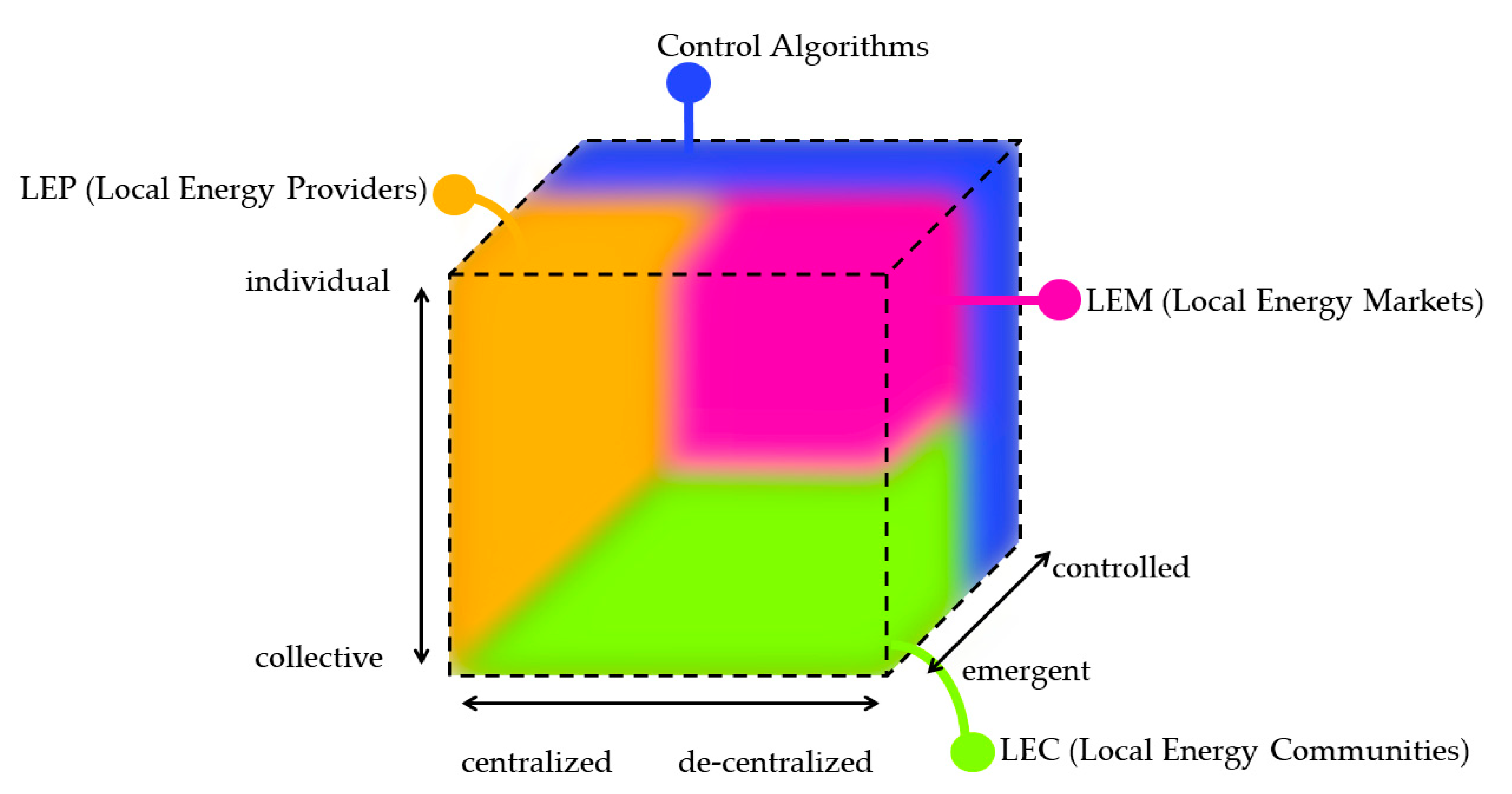
- The examples of business models presented in the study are included in a well-defined search space map (see Figure 3). This facilitates a systematic inquiry and offers a way to organise the results presented in this study and in the follow-ups.
2. Materials and Methods
- (1)
- The controlled versus emergent dimension describes how much there are rules or a controller that directs the exchanges, versus an emergent behaviour from the interactions between agents.
- (2)
- The centralised versus de-centralised dimension describes how much the agents are equivalent among each other, versus the presence of few (potentially one) agents that concentrate some functions for a larger number of others.
- (3)
- The individual versus collective dimension describes how much each agent controls and directs its own resources (i.e., PV, storage, demand-response resources, etc.), versus having larger pools of agents who share some common resources.
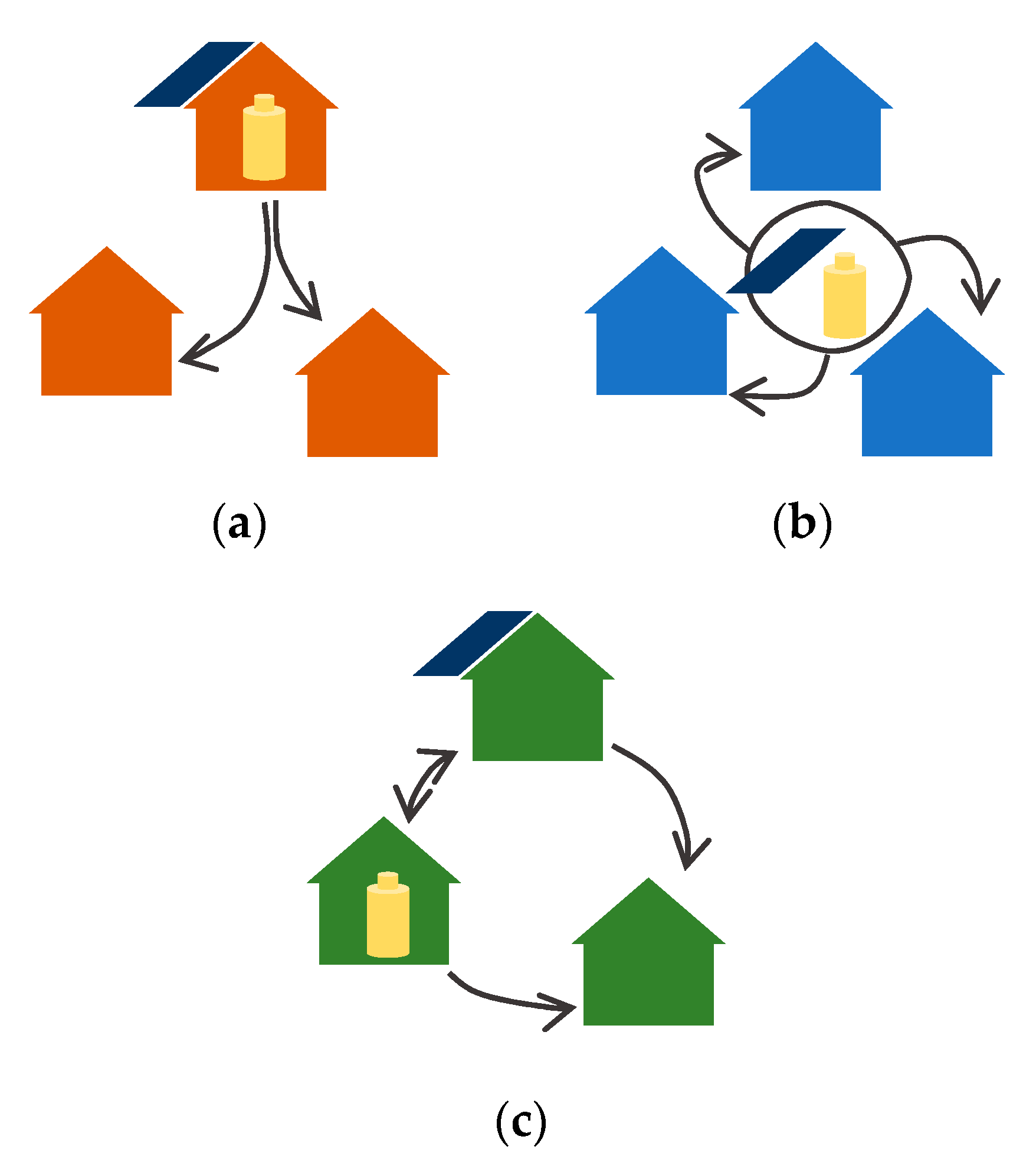
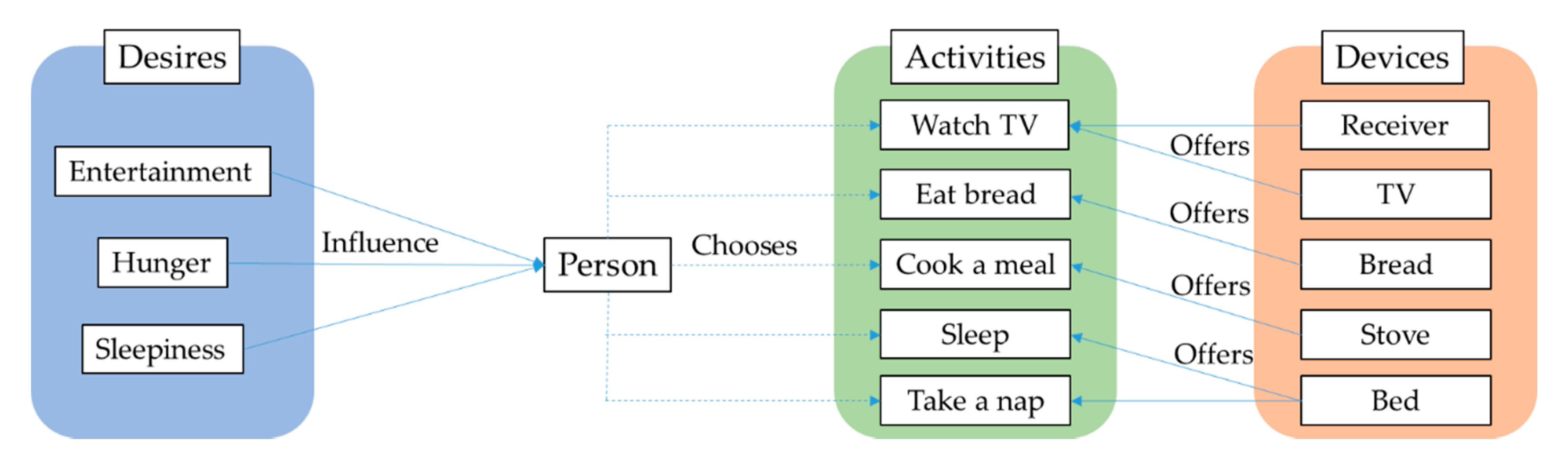
2.1. Agent-Based Model
- Local Energy Provider (LEP) (Figure 4a): It occurs when a single agent owns the totality of the production or storage capacity of the entire local network and the other agents are strictly consumers. The owner of the plant can be either a producer or a prosumer.
- Local Energy Community (LEC) (Figure 4b): It is the case in which a communal plant is shared among all or a group of agents, the shares could be equally distributed or according to other principles such as energy used from the plant or the share of the initial investment.
- Local Energy Market (LEM) (Figure 4c): It is the most complex and free-form of all the structures; it is characterised by the presence of multiple producers, consumers and prosumers. In this arrangement, the interaction between agents can reach significant complexity and the agents could achieve higher earnings by engaging in intelligent behaviours.
2.2. Ownership Structures and Business Models
- LEC gratis: In this arrangement, the electricity from the communal PV plant is given for free when available. All the households participate in the initial investment and in the Operation and Maintenance (O&M) costs of the plant according to equal shares.
- LEC LCOE: In this arrangement, the electricity from the communal PV is given at production cost (i.e., without profit) and the revenues are divided among the shareholders. Although variable shares are possible, in this study, all the households are equal sharers in the LEC (i.e., initial investment and O&M costs, and the revenues are shared equally).
- LEP n%: This arrangement is a pure form of LEP. Thus, the production plant is owned by a single provider who can set the price at its own will. Obviously, the provider cannot set the price higher than that of the parent grid (i.e., the average price for Swedish household consumer as assumed in Section 2.3) as the consumers retain the right to purchase electricity from the cheapest source. In this study, the provider sets the price as half-way between the minimum of the local LCOE and the maximum of the consumer price from the parent grid. More precisely, the provider sets a price at a percentage n so that n = 0 is the LCOE, n = 100 is the price offered by the parent grid and n = 50 is half-way. This set-up is valid under the assumption that the LCOE of the system is lower than the price of the electricity for the consumer. Of course, if this assumption does not hold true, the provider will not be able to charge above market price and will thus operate at the minimum loss.
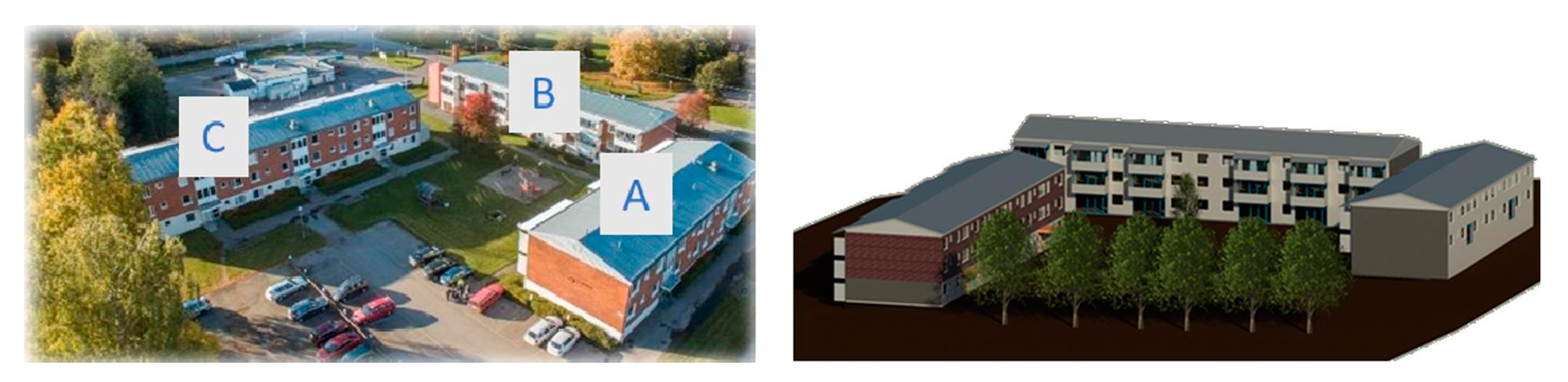
2.3. Case Study
- Local initial price of the turn-key system without taxation: 10,000 SEK/kWp (935 €/kWp).
- Price of the inverter: 2500 SEK/kWp (234 €/kWp) (changed two times over the lifetime). The number of changes was retrieved as the expected value assuming a lifetime of the inverter between 12 and 15 years.
- Planned lifetime of the system: 30 years.
- Maintenance costs for the system (substitutions, cleaning and inspection): 5109 SEK/year (477 €/year). This value was calculated as the expected value out of 100 stochastic simulations.
- Degradation of the performance of the system: ca. −1.15%/year.
3. Results
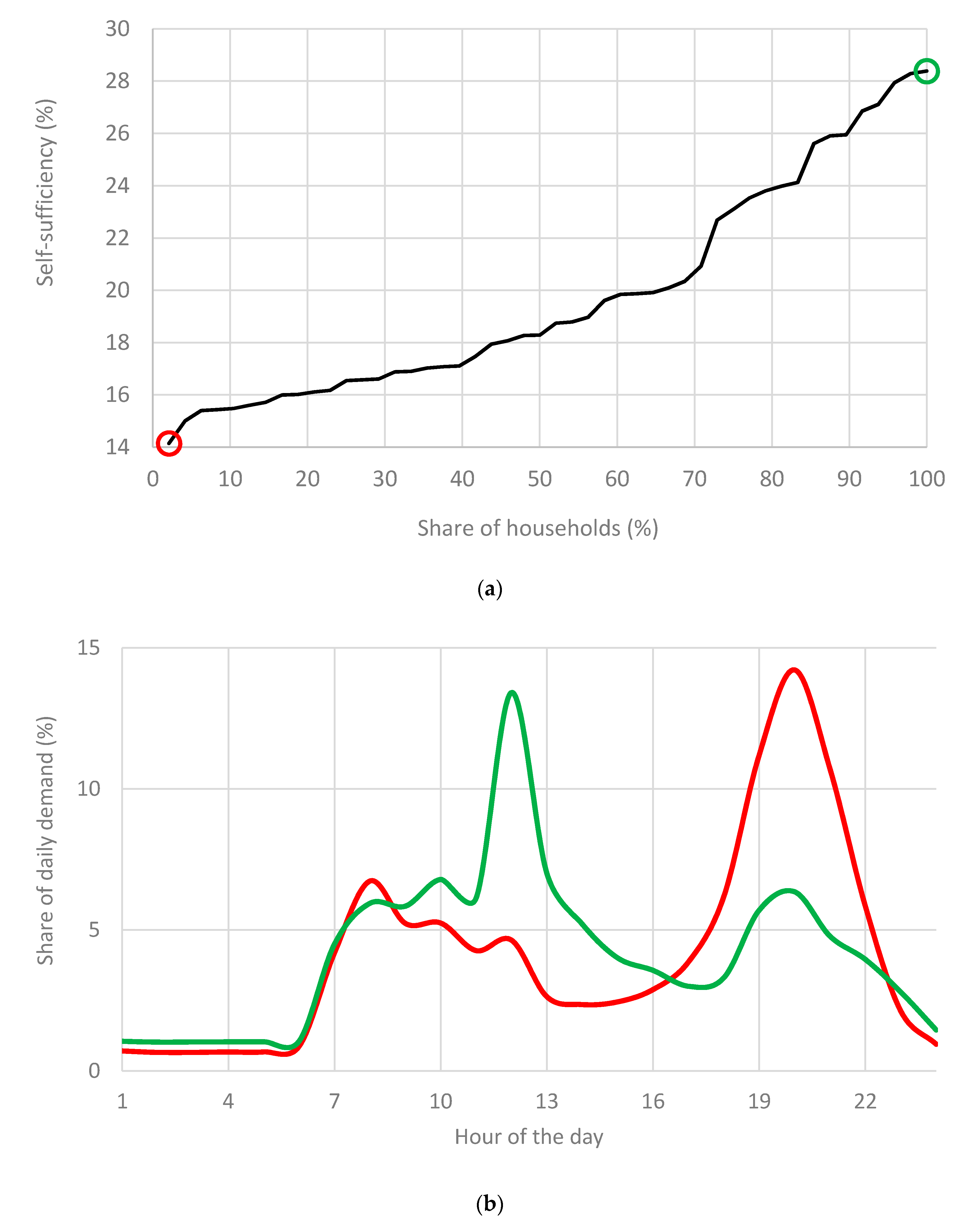
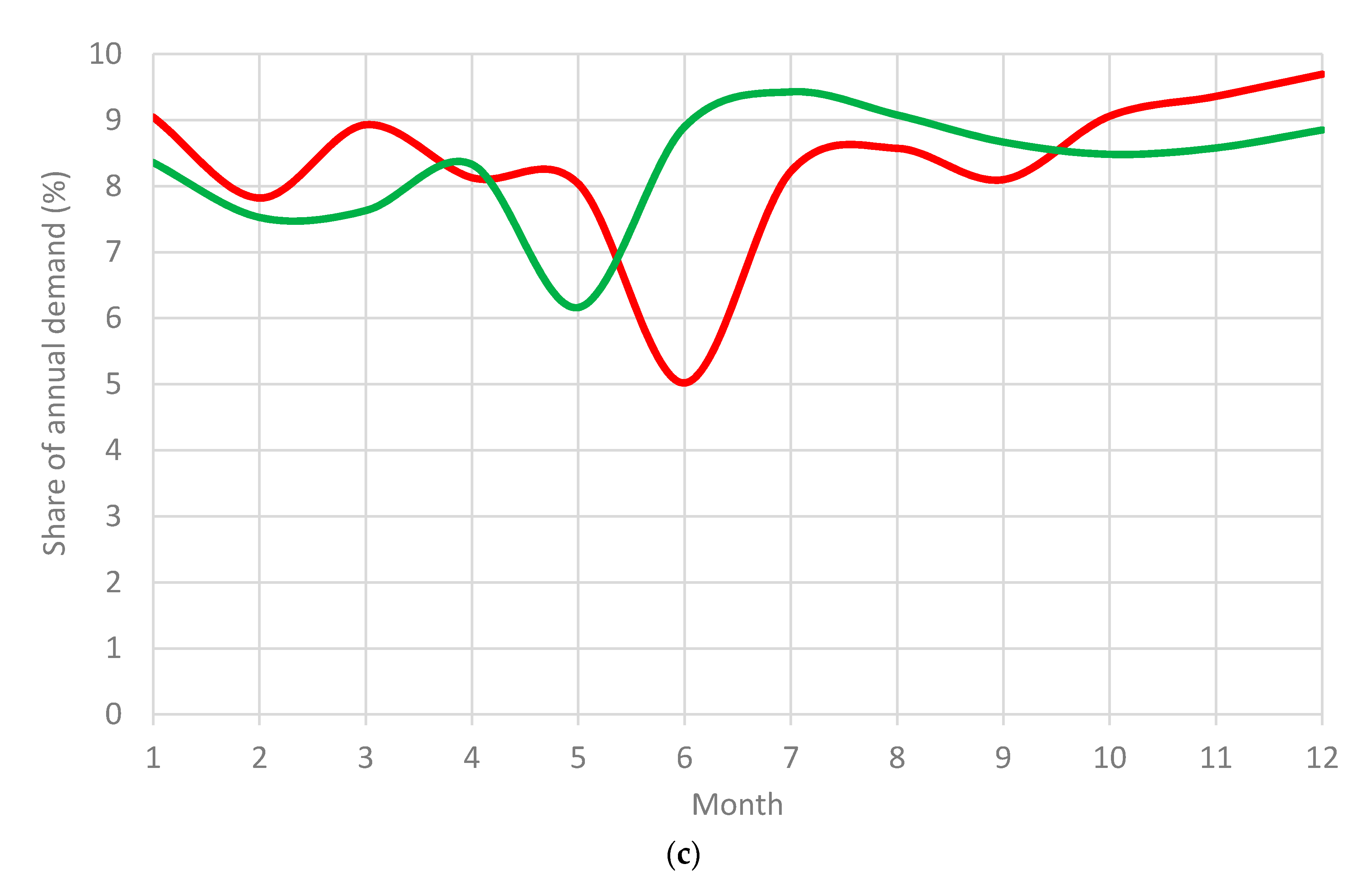
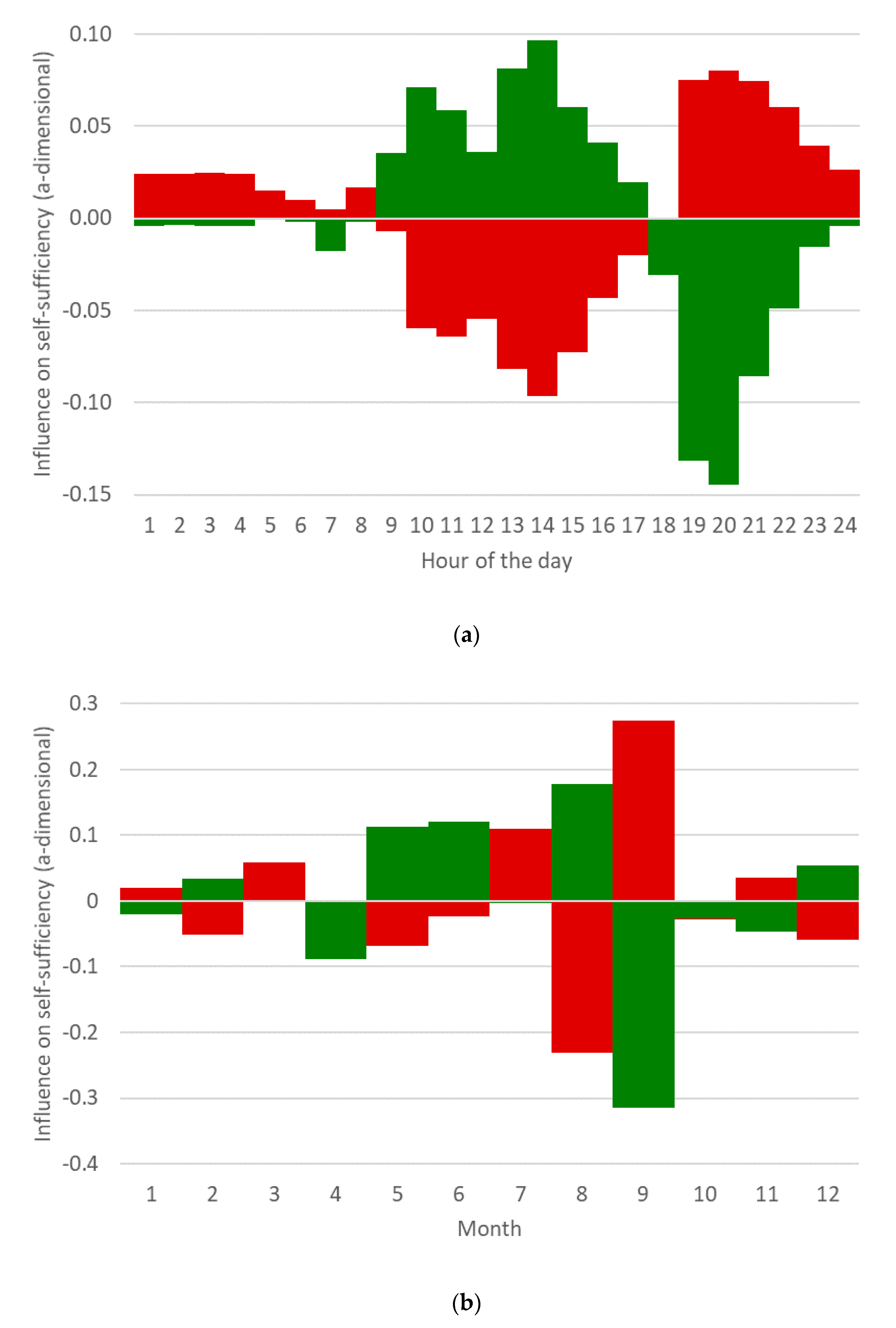
3.1. Self-Sufficiency of the Households
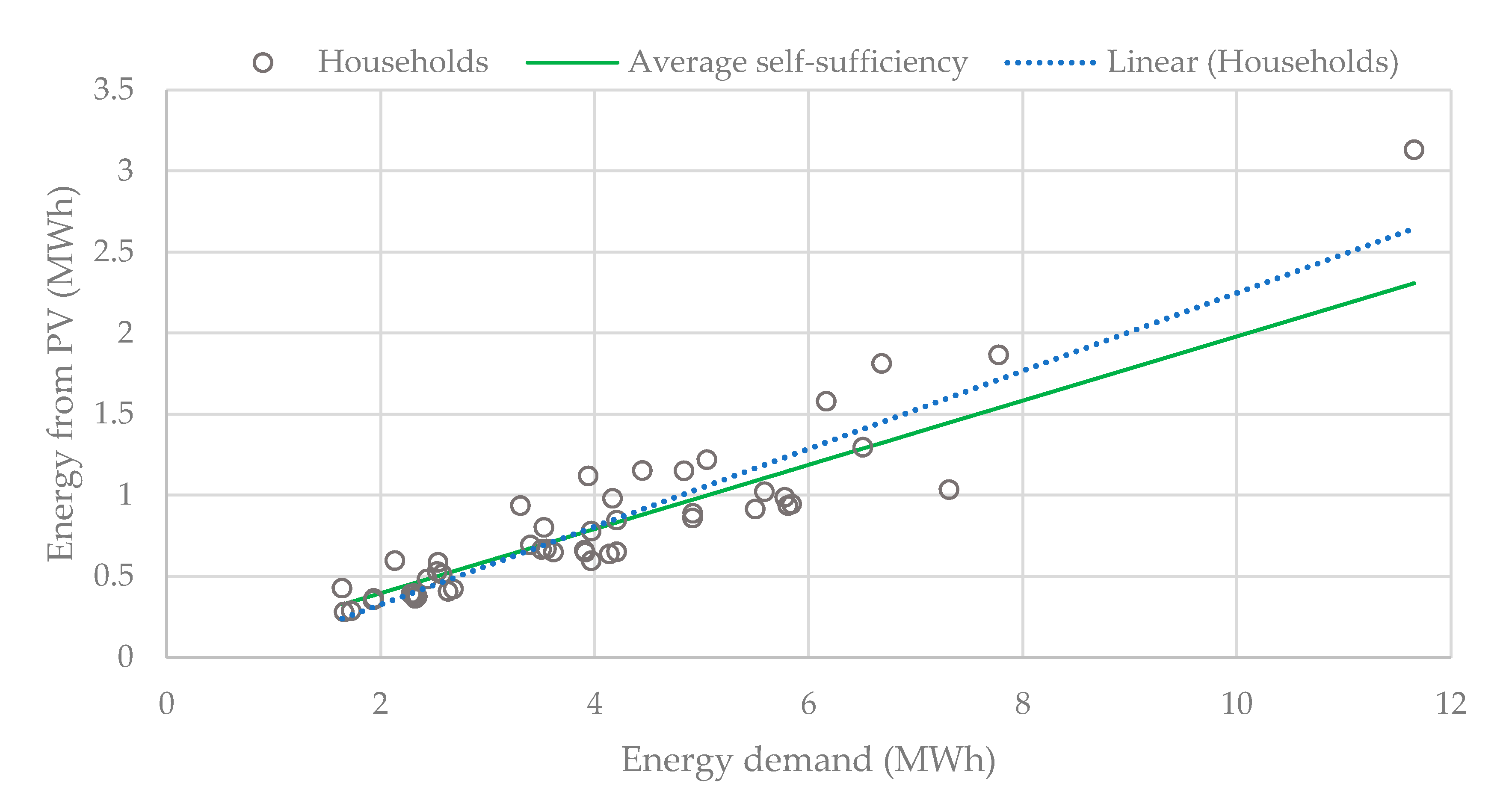
3.2. Exploitation of the Common Renewable Resources: Sheer Cumulative Consumption Versus Self-Sufficiency
3.3. LEC Gratis
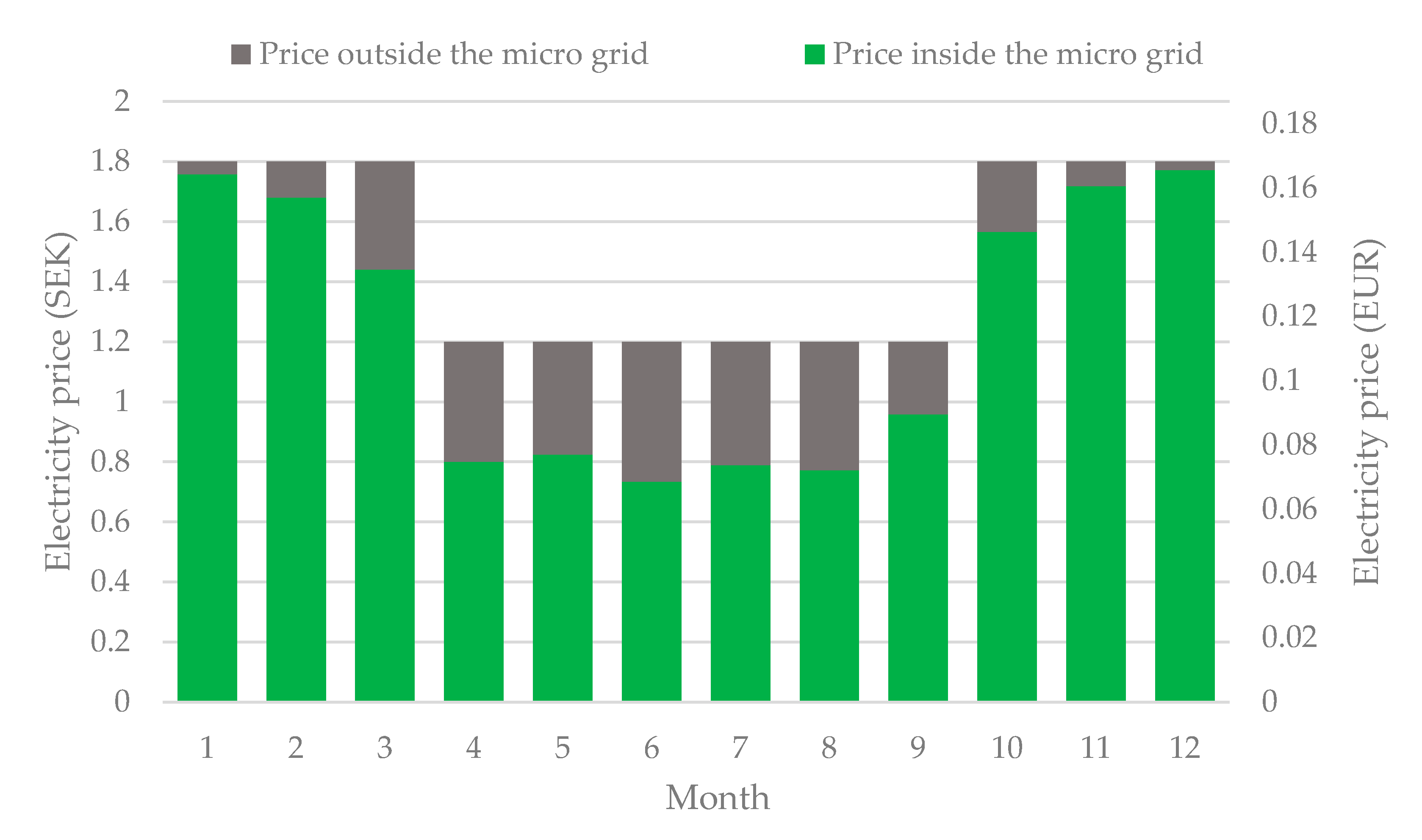
3.4. LCOE of LEC
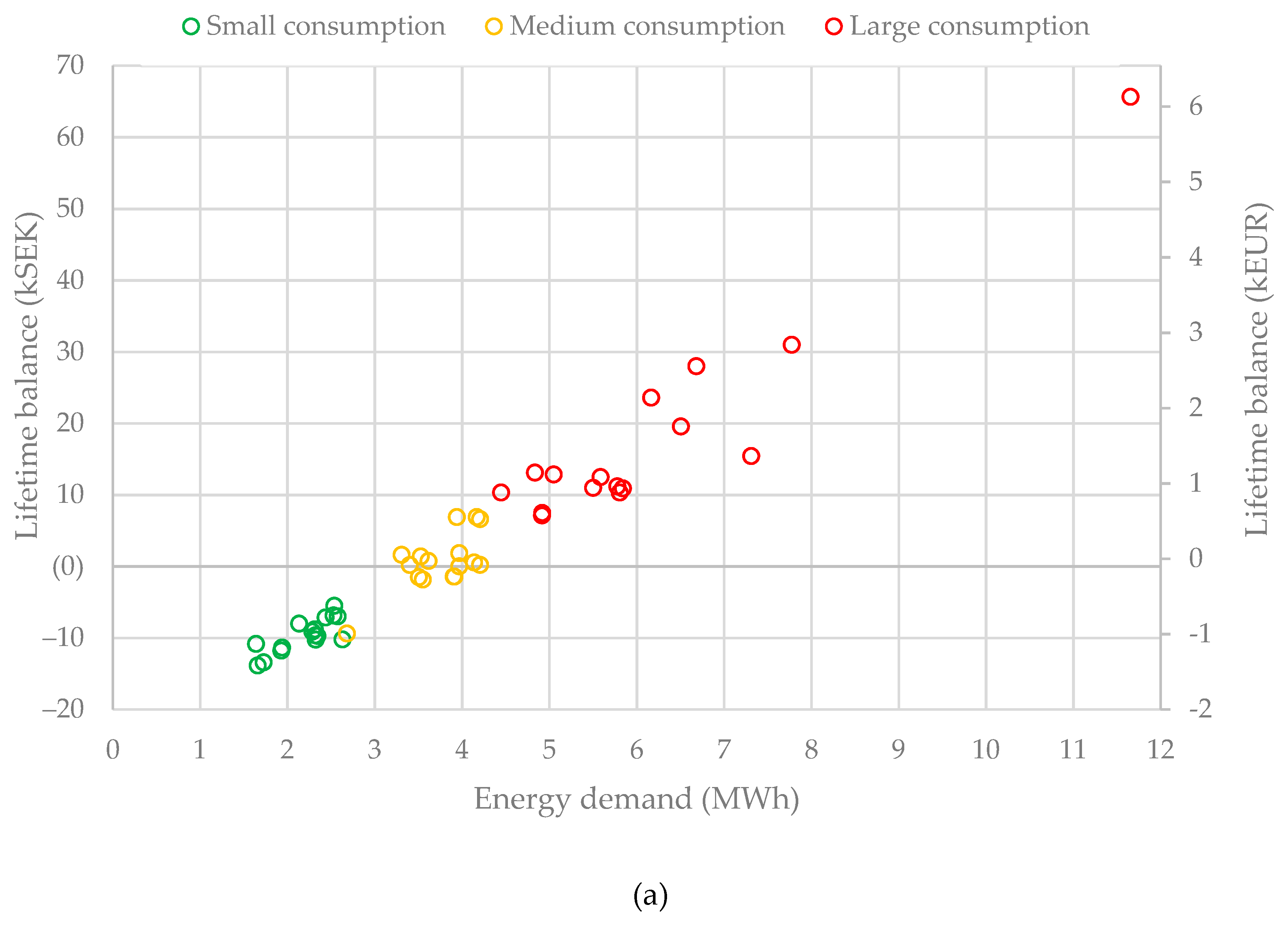
3.5. LEP N%
4. Discussion
4.1. Social and Cultural Differences among Households Have a Huge Impact on Self-Sufficiency
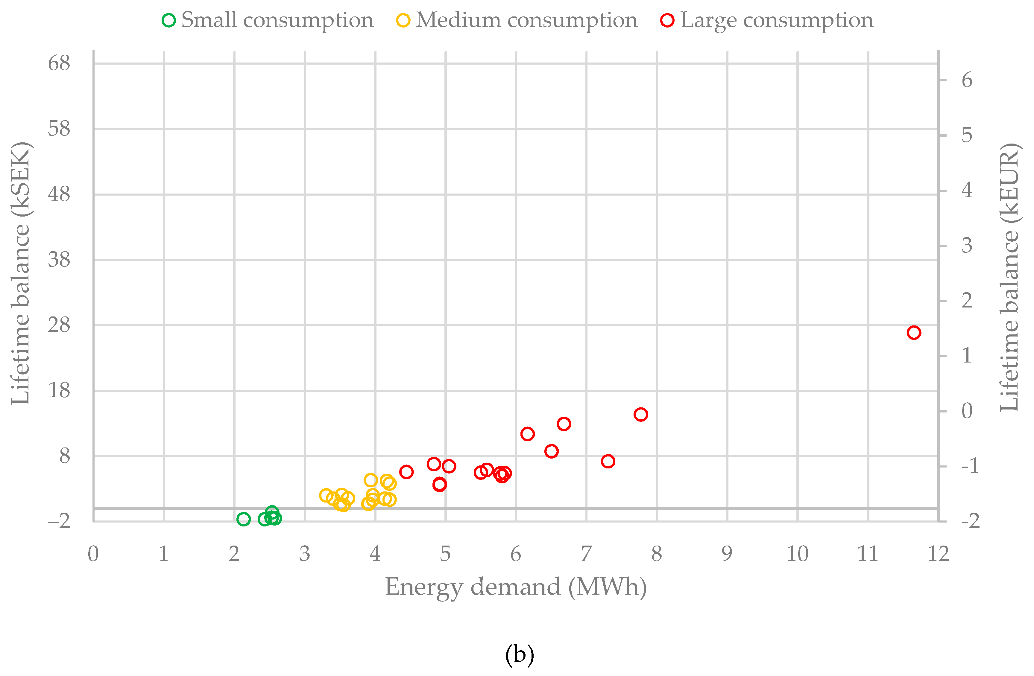
4.2. High Cumulative Energy Demand Is More Effective Than High Self-Sufficiency in Exploiting the Shared Renewable Resource
4.3. Different Selling Prices Generates Various Business Opportunities
5. Conclusions
5.1. Key Findings
- Social and cultural differences among households have a huge impact on self-sufficiency: The households were simulated without introducing any demand-response measure or smart control. However, some households achieved a self-sufficiency of almost 30% using the common PV system while others stopped short of 15%.
- High cumulative energy demand is more effective than high self-sufficiency in exploiting the shared renewable resource: Despite the large differences observed in self-sufficiency among households, the quantity of energy received from the shared system has been determined almost completely by the annual cumulative demand rather than by self-sufficiency.
- Different selling prices generates various business opportunities: Different value of n%, as defined in Section 2.2, generate advantage and interesting features for diverse stakeholders. For instance, a very low n% (i.e., <10%) generates a strong drive for the shareholders to self-consume as much PV energy as possible, but it contains a risk for the least consuming ones. Higher n% (i.e., from ca. 10% to 100%) are interesting for building owners and BIPV solutions and, amid increasing n%, become more and more interesting for third party energy providers.
5.2. Follow-Up Studies
Author Contributions
Funding
Conflicts of Interest
References
- IEA. IEA EBC Annex 83. Available online: https://annex83.iea-ebc.org/ (accessed on 2 June 2020).
- Energimyndigheten. Proposed Strategy for Increased Use of Solar Energy. 2016. Available online: https://energimyndigheten.a-w2m.se/Home.mvc?ResourceId=5599 (accessed on 20 June 2020).
- Huijben, J.; Verbong, G. Breakthrough without subsidies? PV business model experiments in the Netherlands. Energy Policy 2013, 56, 362–370. [Google Scholar] [CrossRef]
- European Commission. Clear Energy Package. Available online: https://ec.europa.eu/energy/topics/energy-strategy/clean-energy-all-europeans_en (accessed on 3 June 2020).
- Riksdag, S. Regulation (2007: 215) on Exemptions from the Requirement for a Network Concession Pursuant to the Electricity Act (1997: 857). Available online: https://www.riksdagen.se/sv/dokument-lagar/dokument/svensk-forfattningssamling/forordning-2007215-om-undantag-fran-kravet-pa_sfs-2007-215 (accessed on 3 June 2020).
- Parag, Y.; Sovacool, B.K. Electricity market design for the prosumer era. Nat. Energy 2016, 1, 16032. [Google Scholar] [CrossRef]
- Lettner, G.; Auer, A.H.; Fleischhacker, D.; Schwabeneder, B.D.; Moisl, F. Existing and Future PV Prosumer Concepts. 2008. Available online: https://www.pvp4grid.eu/wp-content/uploads/2018/08 (accessed on 15 June 2020).
- Stauch, A.; Vuichard, P. Community solar as an innovative business model for building-integrated photovoltaics: An experimental analysis with Swiss electricity consumers. Energy Build. 2019, 204, 109526. [Google Scholar] [CrossRef]
- Roberts, M.B.; Bruce, A.; MacGill, I. A comparison of arrangements for increasing self-consumption and maximising the value of distributed photovoltaics on apartment buildings. Sol. Energy 2019, 193, 372–386. [Google Scholar] [CrossRef]
- Zhang, C.; Wu, J.; Zhou, Y.; Cheng, M.; Long, C. Peer-to-Peer energy trading in a Microgrid. Appl. Energy 2018, 220, 1–12. [Google Scholar] [CrossRef]
- Xu, Z.; Hu, G.; Spanos, C.J. Coordinated optimization of multiple buildings with a fair price mechanism for energy exchange. Energy Build. 2017, 151, 132–145. [Google Scholar] [CrossRef]
- Nguyen, S.; Peng, W.; Sokolowski, P.; Alahakoon, D.; Yu, X. Optimizing rooftop photovoltaic distributed generation with battery storage for peer-to-peer energy trading. Appl. Energy 2018, 228, 2567–2580. [Google Scholar] [CrossRef]
- Jing, R.; Xie, M.N.; Wang, F.X.; Chen, L.-X. Fair P2P energy trading between residential and commercial multi-energy systems enabling integrated demand-side management. Appl. Energy 2020, 262, 114551. [Google Scholar] [CrossRef]
- Lüth, A.; Zepter, J.M.; Del Granado, P.C.; Egging, R. Local electricity market designs for peer-to-peer trading: The role of battery flexibility. Appl. Energy 2018, 229, 1233–1243. [Google Scholar] [CrossRef] [Green Version]
- Rodrigues, D.L.; Ye, X.; Xia, X.; Zhu, B. Battery energy storage sizing optimisation for different ownership structures in a peer-to-peer energy sharing community. Appl. Energy 2020, 262, 114498. [Google Scholar] [CrossRef]
- Tang, Y.; Zhang, Q.; McLellan, B.; Li, H. Study on the impacts of sharing business models on economic performance of distributed PV-Battery systems. Energy 2018, 161, 544–558. [Google Scholar] [CrossRef]
- Basnet, A.; Zhong, J. Integrating gas energy storage system in a peer-to-peer community energy market for enhanced operation. Int. J. Electr. Power Energy Syst. 2020, 118, 105789. [Google Scholar] [CrossRef]
- Huang, P.; Lovati, M.; Zhang, X.; Bales, C.; Hallbeck, S.; Becker, A.; Bergqvist, H.; Hedberg, J.; Maturi, L. Transforming a residential building cluster into electricity prosumers in Sweden: Optimal design of a coupled PV-heat pump-thermal storage-electric vehicle system. Appl. Energy 2019, 255, 113864. [Google Scholar] [CrossRef]
- Thomas, L.; Zhou, Y.; Long, C.; Wu, J.; Jenkins, N. A general form of smart contract for decentralized energy systems management. Nat. Energy 2019, 4, 140–149. [Google Scholar] [CrossRef]
- Alam, M.R.; St-Hilaire, M.; Kunz, T. Peer-to-peer energy trading among smart homes. Appl. Energy 2019, 238, 1434–1443. [Google Scholar] [CrossRef]
- El-Baz, W.; Tzscheutschler, P.; Wagner, U. Integration of energy markets in microgrids: A double-sided auction with device-oriented bidding strategies. Appl. Energy 2019, 241, 625–639. [Google Scholar] [CrossRef]
- Chen, K.; Lin, J.; Song, Y. Trading strategy optimization for a prosumer in continuous double auction-based peer-to-peer market: A prediction-integration model. Appl. Energy 2019, 242, 1121–1133. [Google Scholar] [CrossRef]
- Sousa, T.; Soares, T.; Pinson, P.; Moret, F.; Baroche, T.; Sorin, E. Peer-to-peer and community-based markets: A comprehensive review. Renew. Sustain. Energy Rev. 2019, 104, 367–378. [Google Scholar] [CrossRef] [Green Version]
- Zepter, J.M.; Lüth, A.; Del Granado, P.C.; Egging, R. Prosumer integration in wholesale electricity markets: Synergies of peer-to-peer trade and residential storage. Energy Build. 2019, 184, 163–176. [Google Scholar] [CrossRef]
- Cornélusse, B.; Savelli, I.; Paoletti, S.; Giannitrapani, A.; Vicino, A. A community microgrid architecture with an internal local market. Appl. Energy 2019, 242, 547–560. [Google Scholar] [CrossRef] [Green Version]
- Almasalma, H.; Claeys, S.; Deconinck, G. Peer-to-peer-based integrated grid voltage support function for smart photovoltaic inverters. Appl. Energy 2019, 239, 1037–1048. [Google Scholar] [CrossRef]
- Šúri, M.; Huld, T.; Dunlop, E.D. PV-GIS: A web-based solar radiation database for the calculation of PV potential in Europe. Int. J. Sustain. Energy 2005, 24, 55–67. [Google Scholar] [CrossRef]
- Pflugradt, N.; Muntwyler, U. Synthesizing residential load profiles using behavior simulation. Energy Procedia 2017, 122, 655–660. [Google Scholar] [CrossRef]
- Pflugradt, N.; Teucher, J.; Platzer, B.; Schufft, W. Analysing low-voltage grids using a behaviour based load profile generator. Renew. Energy Power Qual. J. 2013, 361–365. [Google Scholar] [CrossRef]
- Luthander, R.; Widén, J.; Nilsson, D.; Palm, J. Photovoltaic self-consumption in buildings: A review. Appl. Energy 2015, 142, 80–94. [Google Scholar] [CrossRef] [Green Version]
- IEA. Snapshot of Global PV Markets; IEA: Paris, France, 2020. [Google Scholar]
- Lovati, M.; Salvalai, G.; Fratus, G.; Maturi, L.; Albatici, R.; Moser, D. New method for the early design of BIPV with electric storage: A case study in northern Italy. Sustain. Cities Soc. 2019, 48, 101400. [Google Scholar] [CrossRef] [Green Version]


| Block | Facing | Tilt (degree) | Capacity (kWp) | Production (MWh) |
|---|---|---|---|---|
| B | South | 18 | 28.4 | 22 |
| C | East | 18 | 15.9 | 10.4 |
| A | West | 18 | 15.9 | 10.3 |
| A | South | 90 | 5.3 | 3.4 |
| N (%) | Revenues (SEK) | Balance (SEK) | Balance (€) | IRR (%) |
|---|---|---|---|---|
| 0 | 34,553 | −94,058 | −8790 | −0.5 |
| 9.43 | 37,689 | 0 | 0 | 0.0 |
| 25 | 42,864 | 155,247 | 14,509 | 0.7 |
| 50 | 51,174 | 404,553 | 37,809 | 1.6 |
| 75 | 59,484 | 653,859 | 61,108 | 2.3 |
| 100 | 67,794 | 903,165 | 84,408 | 2.9 |
© 2020 by the authors. Licensee MDPI, Basel, Switzerland. This article is an open access article distributed under the terms and conditions of the Creative Commons Attribution (CC BY) license (http://creativecommons.org/licenses/by/4.0/).
Share and Cite
Lovati, M.; Zhang, X.; Huang, P.; Olsmats, C.; Maturi, L. Optimal Simulation of Three Peer to Peer (P2P) Business Models for Individual PV Prosumers in a Local Electricity Market Using Agent-Based Modelling. Buildings 2020, 10, 138. https://0-doi-org.brum.beds.ac.uk/10.3390/buildings10080138
Lovati M, Zhang X, Huang P, Olsmats C, Maturi L. Optimal Simulation of Three Peer to Peer (P2P) Business Models for Individual PV Prosumers in a Local Electricity Market Using Agent-Based Modelling. Buildings. 2020; 10(8):138. https://0-doi-org.brum.beds.ac.uk/10.3390/buildings10080138
Chicago/Turabian StyleLovati, Marco, Xingxing Zhang, Pei Huang, Carl Olsmats, and Laura Maturi. 2020. "Optimal Simulation of Three Peer to Peer (P2P) Business Models for Individual PV Prosumers in a Local Electricity Market Using Agent-Based Modelling" Buildings 10, no. 8: 138. https://0-doi-org.brum.beds.ac.uk/10.3390/buildings10080138