Assessing the Energy Resilience of Office Buildings: Development and Testing of a Simplified Metric for Real Estate Stakeholders

Abstract

Increasing concern over higher frequency extreme weather events is driving a push towards a more resilient built environment. In recent years there has been growing interest in understanding how to evaluate, measure, and improve building energy resilience, i.e., the ability of a building to provide energy-related services in the event of a local or regional power outage. In addition to human health and safety, many stakeholders are keenly interested in the ability of a building to allow continuity of operations and minimize business disruption. Office buildings are subject to significant economic losses when building operations are disrupted due to a power outage. We propose “occupant hours lost” (OHL) as a means to measure the business productivity lost as the result of a power outage in office buildings. OHL is determined based on indoor conditions in each space for each hour during a power outage, and then aggregated spatially and temporally to determine the whole building OHL. We used quasi-Monte Carlo parametric energy simulations to demonstrate how the OHL metric varies due to different building characteristics across different climate zones and seasons. The simulation dataset was then used to develop simple regression models for assessing the impact of ten key building characteristics on OHL. The most impactful were window-to-wall ratio and window characteristics. The regression models show promise as a simple means to assess and screen for resilience using basic building characteristics, especially for non-critical facilities where it may not be viable to conduct detailed engineering analysis.

1. Introduction

Resilience in the context of the built environment is commonly described as the ability to prepare for and adapt to changing conditions and withstand and recover rapidly from disruptions [1]. Increasing concern over higher frequency extreme weather events is driving a push towards a more resilient built environment. In recent years there has been growing interest in understanding how to evaluate, measure, and improve building energy resilience, i.e., the ability of a building to provide energy-related services in the event of a local or regional power outage caused by or coupled with events such as extreme heat and cold, wildfires, earthquakes, hurricanes, and floods [2,3]. Energy-related services include the provision of lighting, heating, ventilation and air conditioning (HVAC), and plug power. The building design community is looking to address these issues in new and retrofit construction; owners and operators need to assess and improve the energy resilience of their buildings, and private-sector intermediaries such as the insurance industry are financially vulnerable to these impacts and are potential partners in loss mitigation [4]. Even in developed countries with a mature and reliable electrical grid, many buildings are subject to power outages due to extreme events. For example, millions of people in California were affected by power outages lasting several days due to wildfires that triggered a precautionary shutdown of some transmission lines. Similarly, extreme winter weather and ice storms in many parts of the United States periodically cause days-long power outages for homes and businesses. Energy resilience is a critical component of overall building resilience, and is distinct from structural resilience, or resilience against human-created threats.

Human safety and health are naturally the first priority driver for resilience. Beyond that, many stakeholders are keenly interested in the ability of a building to provide a safe and comfortable indoor environment to allow continuity of operations and minimize business disruption. Buildings such as offices, retail, food service, and sales, while not mission critical like hospitals and public safety buildings, are subject to significant economic losses should building operations be halted due to a power outage. Financial losses due to disrupted business functions may outweigh any costs associated with structural damage. This was the case for numerous buildings after Hurricane Sandy, where insurance payments for lost business were generally more significant than reconstruction expenses [5,6]. These considerations are increasing the interest in energy resilience from building owners, operators, and insurers.

One of the primary challenges with energy resilience is that this concept is still loosely defined and not well characterized. Resilience is sometimes presented in tandem with large-scale sustainability efforts [7]. Numerous standards and guidelines for occupant comfort and energy efficiency already exist [8], including through the LEED (Leadership in Energy and Environmental Design) rating system’s passive survivability credit [9]. However, there are no widely-accepted aggregate metrics for energy resilience. This paper proposes a simple aggregate metric that serves as a first-order measure of building energy resilience, especially as it relates to business continuity in commercial buildings such as offices.

We first provide a background of the relevant literature. Next, we define and describe the proposed metric. We show the application of the metric in a parametric energy simulation analysis. We then describe the viability of computing the metric based on easily obtainable building features. We conclude with limitations and areas for further research.

2. Background

Much of the literature on building-level metrics for resilience is focused on the continuity of building operations for whole communities during a disruption or disaster [10,11,12]. The literature on energy resilience indicates that there are currently no universally agreed-upon metrics for assessing the energy resilience of individual buildings [13]. Various conceptual frameworks have been developed as methods for strategically organizing relevant resilience priorities and data requirements to inform the most appropriate metrics for determining resilience, including matrices [14], workflow charts [15], and decision trees [16]. However, while these frameworks offer stakeholders an approach to thinking through the process of resilience measurement, they do not include explicit energy resilience metrics for individual buildings. A resilience index developed by [17] quantifies the resilience of a building as a function of “robustness, resourcefulness, and recovery” within the context of maintaining building functionality when faced with unique hazards. An “energy provision” metric developed by [18] assesses the ability of a building to provide energy during a disruption, with more specific metrics including natural/mechanical ventilation potential, air filtration, and daylight coverage. Criteria-based building resilience and sustainability rating systems and certifications, such as LEED [19], RELi 2.0 [20], US Resiliency Council Building Rating System [21], and BREEAM (Building Research Establishment Environmental Assessment Method) [22] aim to assess building resilience mostly through “feature-based” verification [23], which provides a prescriptive path to resilience, but does not necessarily take the form of explicit resilience metrics.

A key concept emerging in building energy resilience is “passive survivability”, which denotes the ability of buildings to keep occupants safe and comfortable during a power outage [24]. “Thermal autonomy” has been proposed to assess a building’s potential to keep occupants at acceptable temperatures, with the metric ultimately consisting of the time occupants are kept in these sufficient thermal conditions [24,25]. Similarly, as another time-based metric, “hours of safety” has been proposed as a metric to assess the potential of a building to keep people safe from extreme cold and heat during a power outage, attributing resilience to the performance of thermal comfort-associated building components, such as insulation [26].

Other approaches for measuring building energy resilience is to group buildings with infrastructure systems by their role in infrastructural resilience [11]. Buildings are viewed as components of the larger power grid system, contributing to grid resilience, citing building energy resilience as a function of grid-connectivity [27]. While metrics used to assess the infrastructural resilience of the built environment may not focus on energy explicitly, considerations for measuring the capacity of key facilities, such as hospitals and hotels, to serve and offer shelter to people in times of need, may have embedded energy resilience implications by looking to the continued functionality of these facilities during power disruptions and grid failure. The GridOptimal metrics proposed by the New Buildings Institute address power availability for buildings, but with a stronger emphasis on the contribution of energy-efficient buildings to the overall efficiency of the grid, with a decarbonized grid as the primary focus [28], and not necessarily the comfort and safety of occupants at the individual-building level.

Focusing on the economic implications of lost access to grid energy for individual buildings, “value of lost load” (VoLL) is proposed as a metric to assess the financial consequences of a power disruption, where a lower VoLL, expressed as “$/kWh”, denotes a lesser degree of financial consequence due to a loss in load served, thus indicating a greater degree of building energy resilience [13]. Similarly, “percent of critical load system can support” is proposed as a metric to quantify the amount of lost grid electricity that can be made up by resilience measures during a power disruption, especially renewable energy systems [29,30]. These metrics are primarily focused on renewable energy as a means to foster building energy resilience and are not easily applicable to passive building features. Certain passive building features, such as external shading and high-performing windows, have shown to have significant potential in mitigating indoor conditions in extreme events [31], but further research is still needed to demonstrate the role of these passive building features as a means to increase energy resilience [32].

Our review suggests that resilience, even when narrowed to building energy resilience, can be viewed and assessed in different ways depending on stakeholder interests and use cases. This calls for a suite of metrics, and indeed it may not be possible or desirable to try and define a single metric for all these use cases. One apparent gap, vis-a-vis building energy resilience, is the emerging need for an aggregate measure of building energy resilience that can be used by owners, investors, operators. While passive survivability is a step in this direction, it is a technical metric that is more oriented towards the design community. In the next section, we build on the concept of passive survivability to propose an aggregate metric for building energy resilience that is targeted towards assessing it from the stance of business continuity for commercial buildings such as offices and retail facilities.

3. Proposed Metric for Energy Resilience in Office Buildings

There are long-standing existing metrics and criteria to evaluate indoor environmental conditions for building occupants. Widely accepted guidance in this area include ASHRAE Standards 55 [33] for thermal comfort, 62.1 and 62.2 [34,35] for ventilation, and 90.1 [36] for the visual environment. While these are important constituent factors of energy resilience, they are not in and of themselves explicitly configured as resilience metrics. They are generally calculated for a single point in space and time. Building-level resilience requires a cumulative measure integrated over space and time (e.g., total degree hours outside of thermal comfort range). We sought to develop an aggregate energy resilience metric that incorporates multiple constituent indoor environmental quality (IEQ) factors (including thermal comfort, visual comfort, ventilation), thereby providing stakeholders with a straightforward assessment of building energy resilience during a power outage. We focused our effort on office buildings, whose operations may not be critical for public safety but may still realize substantial economic consequences due to power outages. For this use case, our prior experience with industry stakeholders suggests that the metric should be relatively easy to comprehend, and should not require significant data, expertise and effort to compute.

We considered two methodological approaches for defining this new building level energy resilience metric: (a) weighted scoring; and (b) productivity impact. In the weighted scoring approach, the metric is essentially a weighted sum of the individual constituent IEQ factors, normalized to a common scale for summation. The weights for each constituent IEQ factor could be varied based on the priorities of the stakeholders. The advantage of this approach is that the aggregate metric directly uses well-established measurable IEQ factors. However, the disadvantages are that the weighting is subjective, and a weighted score itself is an abstract quantity that is not inherently meaningful. The second approach we considered was to develop a metric that more directly captures productivity impact, specifically productivity lost during a power outage. This would be more meaningful for the end-users and could be more easily converted into economic impacts.

Accordingly, we propose an impact-driven energy resilience metric of “occupant hours lost” (OHL) as a means to measure the business productivity lost as the result of a power outage [37]. OHL may be an absolute value (number of occupant-hours lost over a given time period) or proportional (percentage of normal occupancy lost). For example, an office building with 100 occupants working 40 h a week would have a total of 4000 occupant hours per week under normal conditions. If a power outage made the building unusable for 50 occupants for 20 h over the course of a week, the OHL would be 1000 occupant hours or 25%. The primary appeal of this metric is that it is conceptually simple and can be easily understood by building owners and occupants. It can be translated into economic impact by assigning a monetary value to each occupant hour. Additionally, it can be computed at different levels of spatial or temporal resolution (e.g., OHL for one floor or section of a building, OHL for a 3-h power outage during a summer heat event, etc.).

While conceptually simple, the key methodological consideration for computing OHL are the criteria used to determine when a space is no longer usable by the occupant. Simply using the comfort criteria for normal occupancy would be unnecessarily stringent, since most occupants would be willing to tolerate less than comfortable conditions for limited periods of time, especially under exceptional circumstances such as a power outage. Based on our literature review, we defined the tolerance criteria for the standard effective temperature (SET) (SET is the temperature of an imaginary environment with 50% relative humidity, average airspeed less than 0.1 m/s, and mean radiant temperature equal to air temperature [33]). It is used to represent thermal sensation [38] as a proxy for thermal comfort. CO₂ concentration is used as a proxy for ventilation, and illuminance as a proxy for visual comfort. These criteria, shown in

Table 1. Criteria for calculating OHL based on standard effective temperature, CO₂, and illuminance.

IEQ Factor	Criteria	Basis
Thermal-SET	Max 240 °C SET degree-hours between 30–39.4 °C Max 120 °C SET degree-hours between 4.4–12.2 °C	[9]
Ventilation-CO2	Max 40,000 ppm-hours over 8 h, never to exceed 30,000 ppm	[40,41]
Visual-Illuminance	Min 150 lux; 100–150 lux for 1 h max per day	[36]

, are based on existing standards. Note that there are a maximum and minimum as well as a time-weighted tolerance limit within that range. A space would be considered unusable whenever tolerance criteria are not met for a given time interval, and the total occupant-hours in that space over that time period would be considered lost. Users may compute OHL based on each individual IEQ factor or multiple factors simultaneously. We would note that these criteria may not be universally acceptable and may need to be adjusted based on use cases and stakeholder priorities. Our review of the literature on comfort criteria showed a need for further research on human tolerance of uncomfortable indoor environmental conditions and how human physiology and behavioral aspects affect adaptation to these indoor conditions [39], albeit a topic that is largely beyond the scope of building science research, per se. Nonetheless, the criteria presented below serve as a starting point for illustrating the use of OHL. Our criteria for occupancy did not include domestic hot water. As such, domestic hot water in offices is typically needed only for handwashing and dishwashing in kitchenettes (toilets and urinals do not need hot water). Our premise is that in a critical event, occupants will be able to tolerate unheated water for handwashing and dishwashing.

4. How the Metric Performs: A Simulation Analysis

4.1. Approach

We used energy simulation to understand and illustrate how the OHL metric varies due to different building characteristics, across different climate zones and seasons. Additionally, the simulations were used to generate a dataset to develop a simple predictive model for calculating OHL based on building characteristics (described in the next section).

We used the US Department of Energy (DOE) medium office prototype model compliant with ASHRAE 90.1-2007 [42] as the starting point for our analysis. Figure 1 shows the geometry and floor plan for the prototype model, which has a total floor area of 4980 sq.m, three floors, and a rectangular floor plan with an aspect ratio of 1.5. We used a detailed zoning version of the model [43] that has more realistic thermal zoning than the standard prototype model, which only has five zones per floor. The energy models with detailed office zoning are available for OpenStudio energy modeling environment [44]. The detailed zoning version has 65 zones, allowing a more fine-grained assessment of OHL variations in different parts of the building.

We then conducted a parametric analysis for three climates and 10 building characteristics related to the envelope and occupancy. The three climates were hot-humid represented by Houston, Texas; warm-marine represented by San Francisco, California; and cold-humid represented by Chicago, Illinois.

Table 2. Parameter variations of building characteristics. V1–V4 indicate the discrete values that each parameter can have in this analysis.

		Houston				San Francisco				Chicago
Parameter	Unit	V1	V2	V3	V4	V1	V2	V3	V4	V1	V2	V3	V4
Window-to-wall ratio	-	0.2	0.3	0.4	0.5	0.2	0.3	0.4	0.5	0.2	0.3	0.4	0.5
Window glazing type	U-Value (W/m2-K)	2.245	2.254	2.969	5.351	2.245	2.399	2.969	5.351	2.067	2.245	2.969	2.969
	SHGC	0.17	0.27	0.45	0.55	0.27	0.45	0.58	0.71	0.27	0.45	0.50	0.62
	Visible transmittance	0.21	0.40	0.45	0.53	0.40	0.53	0.65	0.74	0.40	0.53	0.58	0.66
Wall insulation	U-Value (W/m2-K)	1.29	0.85	0.7	0.51	1.26	0.70	0.51	0.47	0.88	0.47	0.38	0.33
Wall reflectance	-	0.22	0.3	0.5	0.7	0.22	0.3	0.5	0.7	0.22	0.3	0.5	0.7
Roof insulation	U-Value (W/m2-K)	0.57	0.37	0.28	0.23	0.57	0.37	0.28	0.23	0.4	0.35	0.28	0.18
Roof reflectance	-	0.3	0.55	0.7	0.8	0.3	0.55	0.7	0.8	0.3	0.55	0.7	0.8
Occupancy density	ft2/person	130	200	300	400	130	200	300	400	130	200	300	400
Elec Plug and Process	W/ft2	1.25	1	0.75	0.5	1.25	1	0.75	0.5	1.25	1	0.75	0.5
Orientation	Degrees	0	45	90	-	0	45	90	-	0	45	90	-
Infiltration	10−3 m3/s-m2	0.569	0.797	1.024	1.133	0.569	0.797	1.024	1.133	0.569	0.797	1.024	1.133

shows the list of parameters and the range of values for each. The ranges were determined based on a review of the values used in various vintages of DOE prototype models [45] and reference models [46]. The parameter values for windows, wall insulation, and roof insulation varied by climate to account for different construction practices in those locations. The ranges for other parameters such as occupant density and plug loads were the same across climate zones. HVAC and lighting characteristics are not relevant since the assumption is that there is no power available to run these systems. Since our use case is to assess resilience for business continuity, we included plug loads under the assumption that they could be operated with battery power or onsite non-grid sources.

We used a quasi-Monte Carlo approach for creating parametric cases. This approach is well-suited to this analysis because buildings can have any combination of these parameter values and it is not feasible to model all permutations and combinations. We set up a simulation framework that generated parametric cases by randomly selecting one parameter value from the list of values for each parameter. Each parameter value was selected independently of other parameter values (However, note that window glazing type properties (U-value, SHGC, visible transmittance) were not varied independently. Rather, the glazing type itself was treated as the variable). We generated 500 parametric cases for each climate (We determined 500 simulations to be adequate as follows: after each additional parametric simulation, we calculated the mean of the distribution of site energy. When the standard error of the mean fell below a threshold, we determined that additional parametric simulations were not required).

For each climate and for each parametric case, we ran the simulation and computed OHL for power outage events for five week-long periods with different outdoor temperature conditions, using the TMY weather files for the representative locations. We selected these “weather weeks” based on the average temperature from 8 a.m.–6 p.m. for each week:

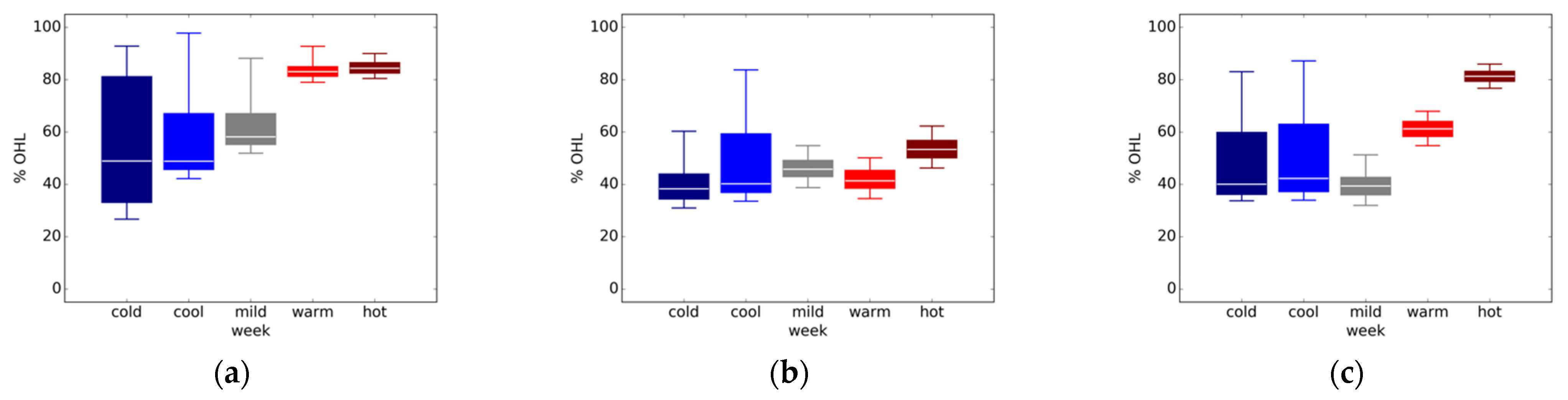
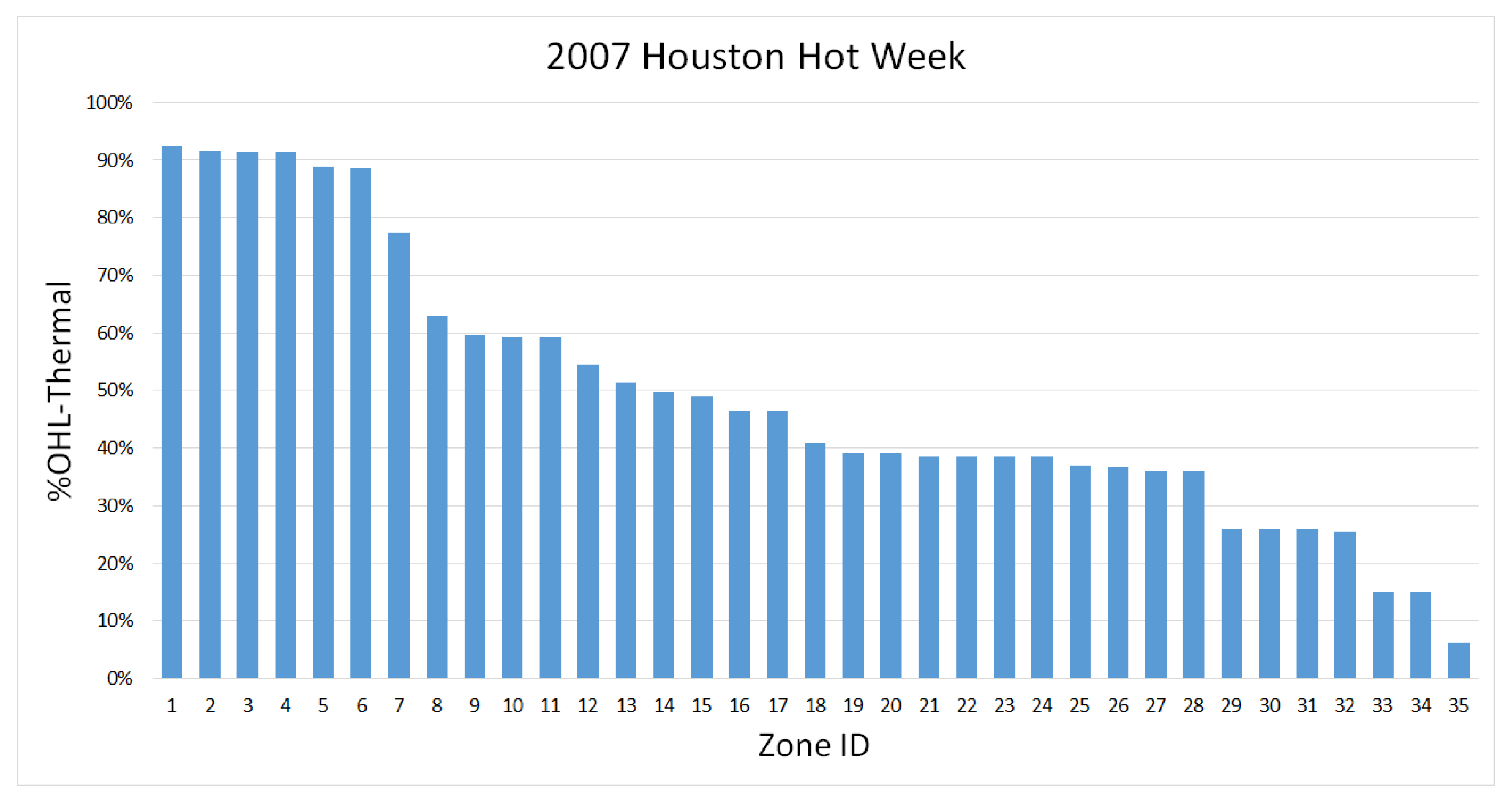
• Hot weather week: the week with highest average temperature.
• Cold weather week: the week with lowest average temperature.
• Mild weather week: the week with the median average temperature.
• Cool weather week: the week with 25th percentile of average temperature.
• Warm weather week: the week with 75th percentile of average temperature.

In each parametric simulation run, we ran the building with normal operations for the week prior to the weather week before “shutting off” HVAC and lighting for the weather week. This ensured that any thermal mass effects from normal operations in the prior week would be accounted for in the weather week.

We computed four OHL metrics from the simulation output for each parametric case, using the criteria described earlier:

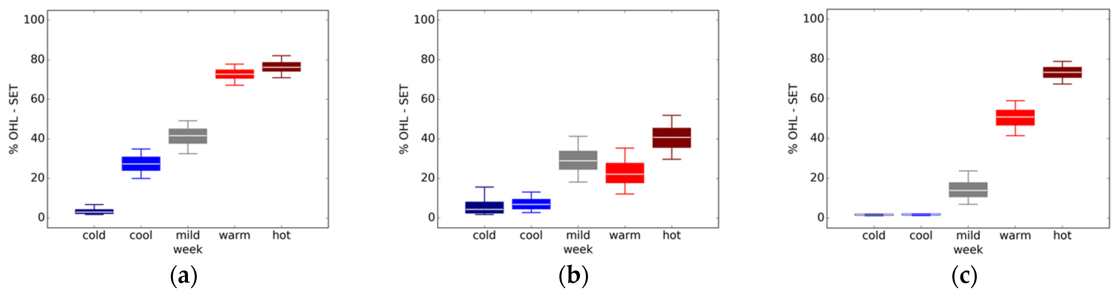
• Thermal OHL was calculated from the hourly standard effective temperature (SET) and occupancy in each zone. It represents the building’s ability to maintain thermal habitability without HVAC systems.
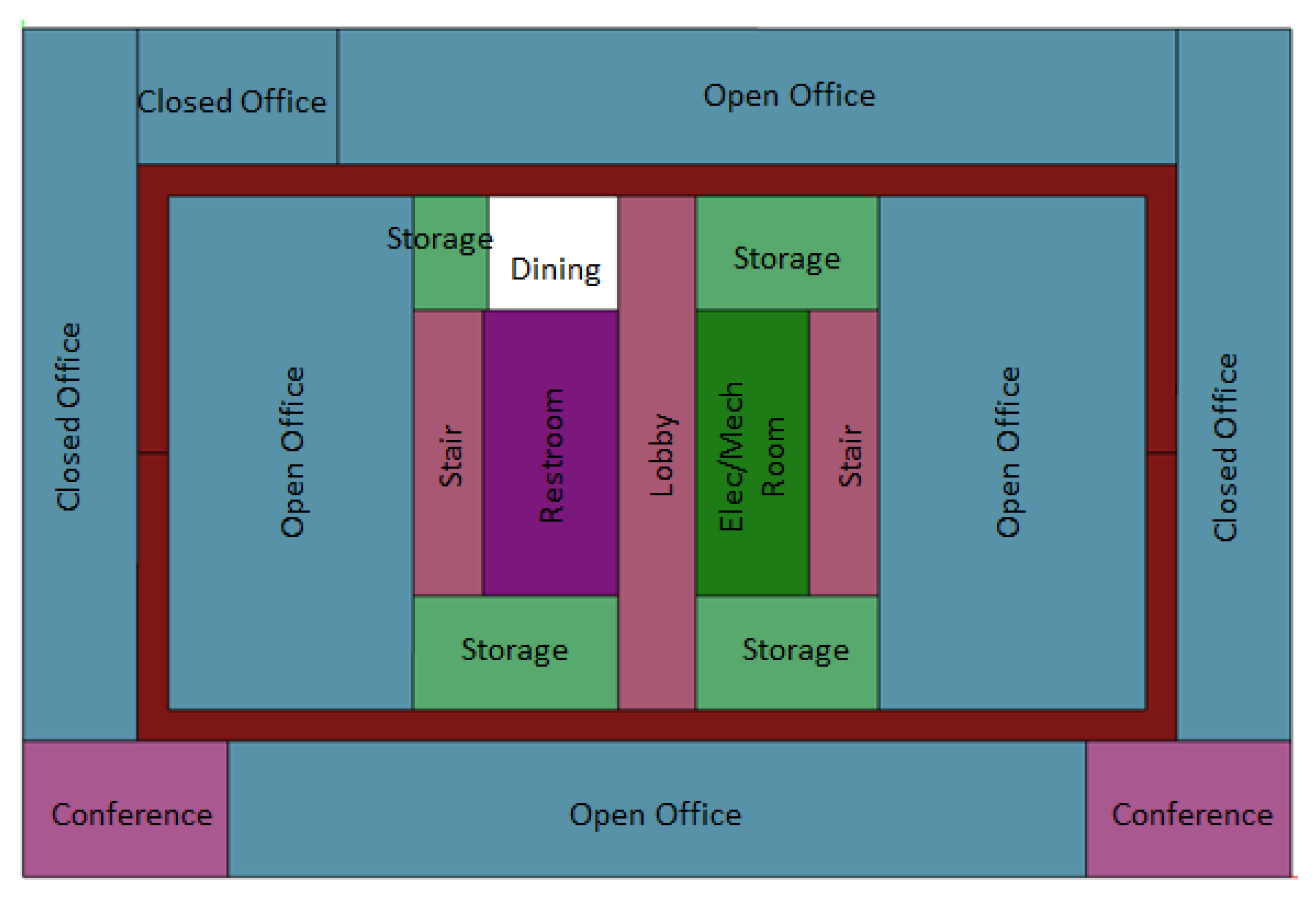
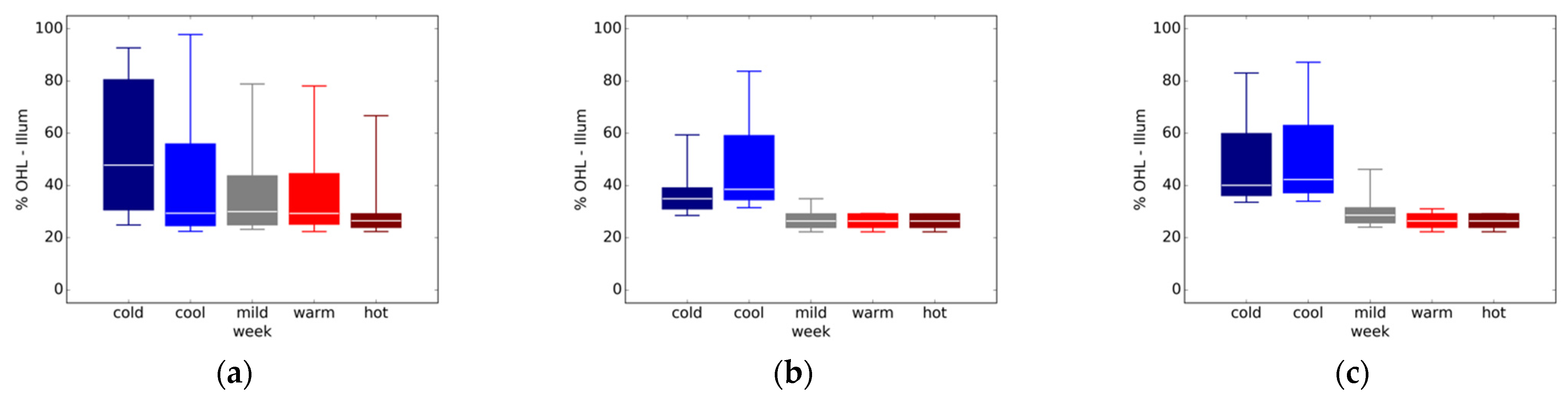
• Visual OHL was calculated from hourly illuminance and occupancy in each zone. It represents the building’s ability to provide adequate daylighting. The illuminance was calculated at a distance of 3 m from the window. (Illuminance is 0 lux in zones without windows.)
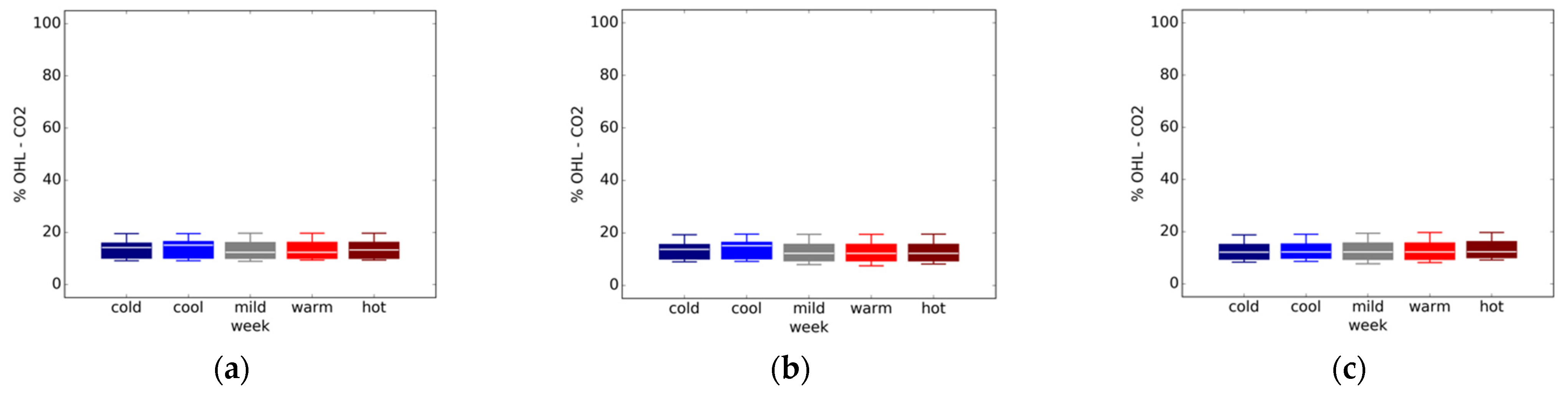
• Ventilation OHL was calculated from the hourly CO₂ concentration and occupancy in each zone. It represents the building’s ability to maintain tolerable CO₂ levels without mechanical ventilation.
• Overall, OHL was calculated using hourly SET, illuminance, CO₂ concentration, and occupancy in each zone. It represents the building’s ability to maintain overall indoor environmental quality without active HVAC and electrical lighting.

OHL was calculated for each hour for each zone and then aggregated to compute the building level OHL for each weather week.

4.2. Results and Discussion

Figure 2, Figure 3, Figure 4 and Figure 5 show the thermal, visual, ventilation, and overall OHL, respectively. Each chart shows the OHL for the five event weeks. The OHL range for each event week is represented by a box plot showing the median, 25th, and 75th percentile (lower and upper bound of the box) and 5th and 95th percentile (lower and upper bounds of the line). A few key observations:

• Thermal OHL: Thermal OHL was highest in the hot weather week for all three locations and generally increased from cold to hot weather weeks. There was a wide range on OHL across weather weeks-about 60% in Houston and Chicago and 40% in San Francisco, which has a milder climate. Thermal OHL was low in cold and cool weather weeks, which could be attributed to solar gain and internal loads. The 5th–95th percentile range of OHL is generally consistent at about 20%.
• Visual OHL: In all locations, the lower bound was generally about 20% OHL. This was due to the internal zones that do not receive any daylight. OHL was higher in cool and cold weeks, which can be attributed to less daylight in winter.
• Ventilation OHL: There was very little variation across locations, weather weeks and within weather weeks. This was somewhat to be expected as the only parameters affecting CO₂ level in our simulation model are the infiltration rate and occupant density.
• Overall OHL: This takes into account the combined effect of SET, illuminance, and CO₂ criteria. As a result, the overall OHL ranges are higher than with just the individual criteria. The ranges were fairly consistent across the different climates. Lower bounds are generally around 50%.

The range of variation of the OHL metric suggests that it is broadly responsive and sensitive to weather, climate, and building characteristics; furthermore, it can be simulated and calculated with well-established existing building energy simulation approaches and tools.

The results also show the value of multiple OHL metrics. While overall OHL represents the “bottom line” in terms of building usability, the constituent metrics suggest how to prioritize interventions. For example, consider cold and cool weather weeks, where thermal OHL is low. The overall OHL is high primarily due to high visual OHL. Therefore, limited back-up power used for lighting could significantly lower visual OHL and thereby improve overall OHL.

Finally, we would note that OHL varied significantly across different zones in the building. For example, Figure 6 shows the thermal OHL in different zones for a hot weather week in Houston, which ranges from 6–92%. While our analysis and results in this paper focus on building level OHL, some stakeholders may be interested in analyzing zone level OHL to inform and prioritize building resilience interventions. OHL metrics allow for such analyses since they can be computed at various levels of spatial and temporal aggregation.

5. Impact of Building Characteristics-Simplified Predictors

5.1. Approach

The previous section demonstrated how OHL can be calculated using conventional building simulation approaches. However, in practice, such simulation is not feasible for most buildings because of the level of effort to develop simulation models, especially for existing buildings where data collection is more challenging than new construction. This level of effort may be justifiable for large or critical facilities but not for small and medium offices, retail, food service, and sales, etc. For such buildings, owners and operators, insurance providers, and other stakeholders need simple ways to assess resilience and identify opportunities to improve it.

Toward that end, we sought to identify whether OHL impacts could be reasonably estimated using selected building characteristics that are relatively easy to obtain. We conducted conventional multivariate regression analysis on the parametric simulation dataset. The dependent variable was OHL. The independent variables were the building parameters listed in Table 2. We conducted a regression analysis for each location and weather week, and for each of the OHL metrics. Using the resulting regression coefficients for each parameter, we computed the incremental change in OHL for a given change in the parameter value. This, in essence, provides a measure of the impact of changing a building characteristic, all else being equal. We computed these only for parameter coefficients that were significant (p < 0.05).

5.2. Results and Discussion

Table A1. Overall OHL Regression results.

Case	(Intercept)	WWR	Window U-Value	SHGC	Window vis Trans	Wall U-Value	Wall Reflectance	Roof U-Value	Roof Reflectance	Occupant Density	Plug Load Density	Orientation	Infiltration	Adj. R2
HO_hot	0.83408	0.03258	0.01388		−0.07762		−0.02213			−0.00011	0.03387		−42.78699	0.45
HO_warm	0.92863	−0.2135	0.01243		−0.18979		−0.02098			−0.00006	0.03733		−52.55214	0.60
HO_mild	1.08953	−0.52308			−0.32909	−0.02642	−0.03222	−0.04184			0.04		−75.51234	0.66
HO_cool	1.24251	−0.94812		−0.14597	−0.49549	−0.02693						0.0002	−54.39543	0.74
HO_cold	1.45032	−1.30297		−0.20264	−0.61161							0.00052	−62.88679	0.91
SF_hot	0.49055	0.1106	−0.00378	0.20627		−0.01798	−0.03146		−0.02909	0.00014	0.03834	−0.00011	−82.40585	0.86
SF_warm	0.47934	0.03852	−0.0039	0.14003	−0.02844	−0.01556	−0.02002		−0.019	0.00012	0.02267	−0.00006	−68.46596	0.75
SF_mild	0.54614	−0.02084	−0.00611	0.15431	−0.06185	−0.01917	−0.02193		−0.02123	0.00014	0.02662		−85.18133	0.58
SF_cool	1.18469	−0.94152	0.00917		−0.37309							0.00026	−97.10029	0.75
SF_cold	0.89833	−0.44449			−0.24912					0.00005			−91.64591	0.59
CH_hot		0.2105		0.21418	−0.02716	0.01269	−0.02258		−0.01302	−0.00004	0.04047		−47.30604	0.93
CH_warm	0.6362	0.0686	−0.00582	0.21087	−0.05392	−0.01205	−0.02251		−0.02384	0.00005	0.05084	−0.00011	−116.26643	0.80
CH_mild	0.67858	−0.23871		0.0425	−0.14708					0.00008	0.01271	−0.00011	−78.58245	0.49
CH_cool	1.20039	−1.0896	0.02222	−0.07286	−0.35689					−0.00006		0.00037	−68.84239	0.80
CH_cold	1.11705	−0.92302	0.02408	−0.07637	−0.2991							0.00024	−89.11845	0.76

Only coefficients with p <= 0.05 shown; Bold values indicate coefficients with p <= 0.001.

,

Table A2. Thermal OHL Regression results.

Case	(Intercept)	WWR	Window U-Value	SHGC	Window Vis Trans	Wall U-Value	Wall Reflectance	Roof U-Value	Roof Reflectance	Occupant Density	Plug Load Density	Orientation	Infiltration	Adj. R2
HO_hot	0.46288	0.19311	0.01085	0.17596	0.01308	0.01685	−0.03929	0.01713	−0.02466	−0.00007	0.07828		−16.13206	0.96
HO_warm	0.39134	0.1672	0.00803	0.17036	0.01103	0.00651	−0.03564	0.01578	−0.0311	−0.00002	0.10329		−31.14112	0.95
HO_mild	0.26186	0.0858		0.18575		−0.02694	−0.0499	−0.04036	−0.04495	0.00007	0.12178	−0.00034	−36.94327	0.92
HO_cool	0.16342	0.04988	−0.00556	0.17479		−0.02755	−0.04252	−0.03851	−0.0349	0.00014	0.09769	−0.00011	−44.32564	0.95
HO_cold	0.06712	−0.01553	−0.00668	0.07686		−0.02687	−0.01709	−0.02209	−0.00816	0.00002	0.04315	−0.00019	−23.56909	0.80
SF_hot	0.15529	0.21074	−0.00787	0.31341	0.04525	−0.02816	−0.05604	−0.01564	−0.06407	0.00022	0.10004	−0.00009	−71.31831	0.92
SF_warm	0.0463	0.16941	−0.01434	0.32515	0.05845	−0.04158	−0.06122	−0.02708	−0.06222	0.00021	0.08901		−67.35553	0.93
SF_mild	0.10439	0.15976	−0.01603	0.31604	0.05331	−0.04013	−0.05767	−0.02539	−0.06465	0.00023	0.09244	0.00004	−66.50788	0.94
SF_cool	0.09911	−0.03505	−0.02001	0.11755	0.02586	−0.03813	−0.01628	−0.04688	−0.01418	0.00004	0.067	−0.00021	−31.1346	0.91
SF_cold		0.16269	−0.0154	0.27486	0.03355	−0.04017	−0.03666	−0.04179	−0.01769	0.00013	0.05636	−0.00093	−26.46278	0.86
CH_hot	0.4202	0.25897		0.25586	−0.01936	0.01853	−0.03022	0.01548	−0.02228	0.00002	0.07217	0.00004	−42.18851	0.93
CH_warm	0.29996	0.19879	−0.01792	0.3201		−0.0185	−0.03904		−0.04701	0.0001	0.11495	−0.00015	−82.49559	0.90
CH_mild	0.09487	0.11318	−0.03483	0.31584		−0.06512	−0.0325	−0.08057	−0.02433	0.00017	0.08979	−0.00049	−56.3568	0.91
CH_cool	0.01239	0.00808	−0.00243	0.01441		−0.00385				0.00003	0.00301	−0.00004	−5.49333	0.59
CH_cold	0.01152		−0.00068	0.00157		−0.00087			0.00039	0.00003	0.00067	0	−0.64141	0.93

Only coefficients with p <= 0.05 shown; Bold values indicate coefficients with p <= 0.001.

,

Table A3. Ventilation OHL Regression results.

Case	(Intercept)	WWR	Window U-Value	SHGC	Window Vis Trans	Wall U-Value	Wall Reflectance	Roof U-Value	Roof Reflectance	Occupant Density	Plug Load Density	Orientation	Infiltration	Adj. R2
HO_hot	0.51231		−0.00222	0.01725						0.00018			−153.14466	0.92
HO_warm	0.41364									0.00018			−121.63163	0.97
HO_mild	0.43035									0.00019			−118.99631	0.97
HO_cool	0.37269									0.00007			−114.66429	0.93
HO_cold	0.37384	0.00639								0.00008			−118.26842	0.95
SF_hot	0.35438									0.00011		−0.00002	−88.57826	0.94
SF_warm	0.32633		0.00058							0.00008	−0.00185		−72.60319	0.92
SF_mild	0.36495									0.0001			−109.3139	0.94
SF_cool	0.35865									0.00006			−103.42958	0.91
SF_cold	0.37906		0.00113		−0.00806					0.00012		0.00003	−100.15798	0.93
CH_hot	0.35451					−0.00444				0.00012			−87.22699	0.87
CH_warm	0.41193									0.00016			−131.37983	0.96
CH_mild						−0.00246				0.0001			−83.56577	0.92
CH_cool	0.32165	0.00737	0.0022							0.00003			−79.93948	0.86
CH_cold	0.36489					−0.00368				0.00008			−101.5246	0.92

Only coefficients with p <= 0.05 shown; Bold values indicate coefficients with p <= 0.001

and

Table A4. Visual OHL Regression results.

Case	(Intercept)	WWR	Window U-Value	SHGC	Window Vis Trans	Wall U-Value	Wall Reflectance	Roof U-Value	Roof Reflectance	Occupant Density	Plug Load Density	Orientation	Adj. R2
HO_hot	0.68788	−0.34306	0.01929	−0.3148	−0.29769					−0.0003			0.43
HO_warm	1.02647	−0.88035	0.01222	−0.28549	−0.5045					−0.00027			0.78
HO_mild	1.11223	−0.95341		−0.20389	−0.59517					−0.00025		0.00025	0.70
HO_cool	1.35684	−1.389		−0.28819	−0.70917					−0.00022		0.00051	0.75
HO_cold	1.58249	−1.75991		−0.26366	−0.82182					−0.00017		0.00078	0.91
SF_hot	0.35566	−0.04015	0.00182	0.01444	−0.05929					−0.00025			0.85
SF_warm	0.3677	−0.05239	0.00221	0.02056	−0.07871					−0.00025			0.79
SF_mild	0.42582	−0.13533	0.00456		−0.14755					−0.00024		0.00009	0.54
SF_cool	1.20394	−1.22743	0.0119		−0.49739					−0.00022		0.00033	0.78
SF_cold	0.82707	−0.64687	0.00867		−0.34265					−0.00025			0.64
CH_hot	0.32589	−0.01696	0.00288		−0.01717					−0.00025			0.94
CH_warm	0.38083	−0.09991	0.00875		−0.07705					−0.00025			0.76
CH_mild	0.56812	−0.38237	0.0189		−0.21743					−0.00025			0.60
CH_cool	1.21665	−1.34897	0.02706	−0.08916	−0.42726					−0.00021		0.00043	0.80
CH_cold	1.10494	−1.20215	0.03392	−0.10789	−0.384					−0.00022		0.00037	0.78

Only coefficients with p <= 0.05 shown; Bold values indicate coefficients with p <= 0.001

in the Appendix A contain results of the regression for overall OHL, thermal OHL, ventilation OHL, and visual OHL, respectively, showing coefficient values and significance for each parameter for each location and weather week. Figure 7, Figure 8, Figure 9, Figure 10, Figure 11, Figure 12, Figure 13, Figure 14, Figure 15 and Figure 16 show the impacts of selected individual parameters on the relevant OHL metrics, only showing values that were statistically significant (p < 0.05). For each parameter, we calculated the OHL impact of a unit change in the value of that parameter, simply multiplying the unit change by the regression model coefficient for that parameter. We used a unit change that would be meaningful in the context of the general range of values for each parameter.

The impacts vary considerably by location as well as weather week. We offer the following key observations:

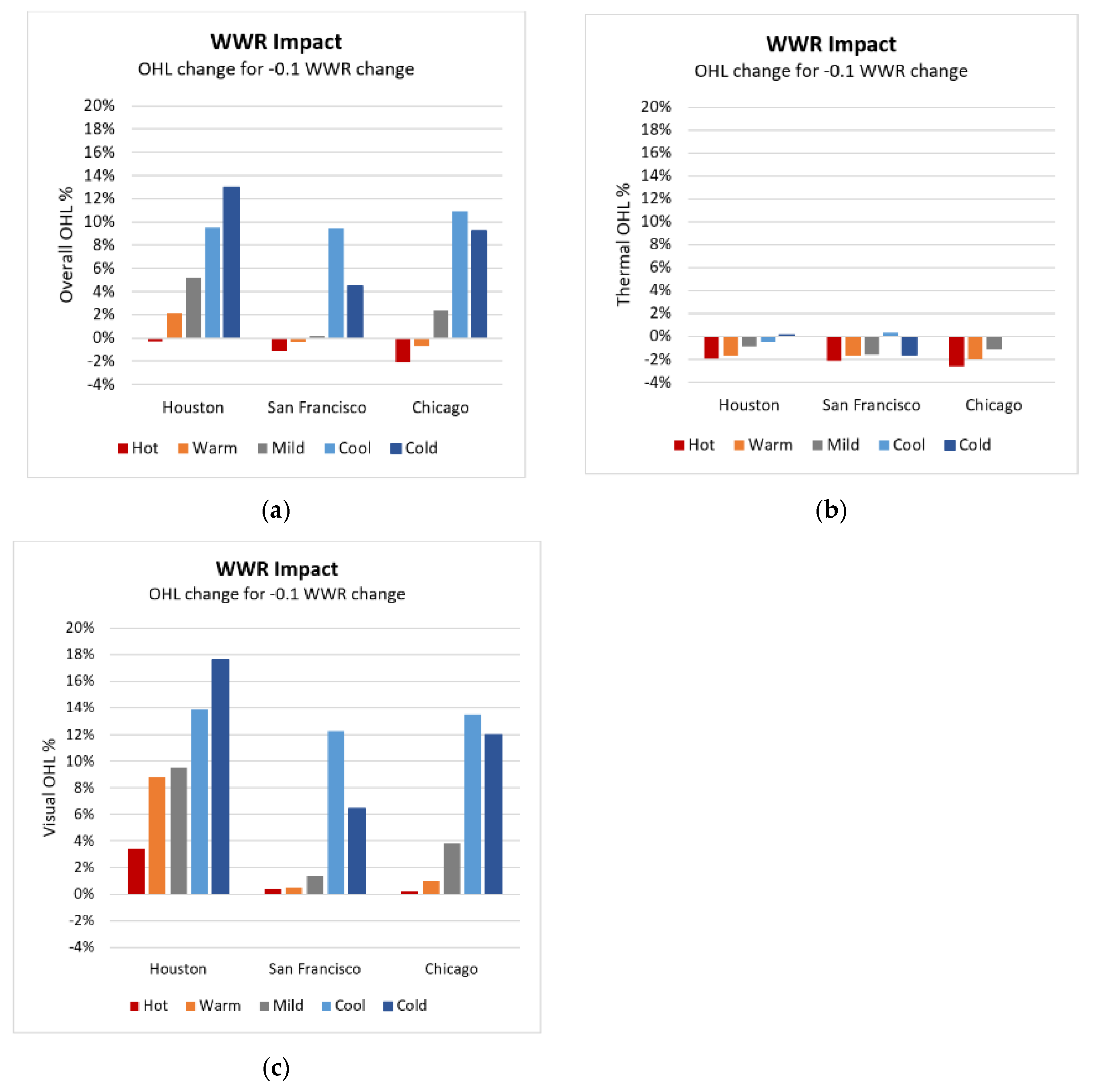
• For WWR, as expected, visual OHL increases while thermal OHL generally decreases with a decrease in WWR. But the impact on visual OHL is an order of magnitude higher than the impacts on thermal OHL, especially in cool and cold weeks, and this, in turn, is reflected in the overall OHL. For example, in Houston WWR impact on thermal OHL ranges from about −2.6% to +0.4%, while WWR impact on visual OHL ranges from about 0.2 to 17.6%.
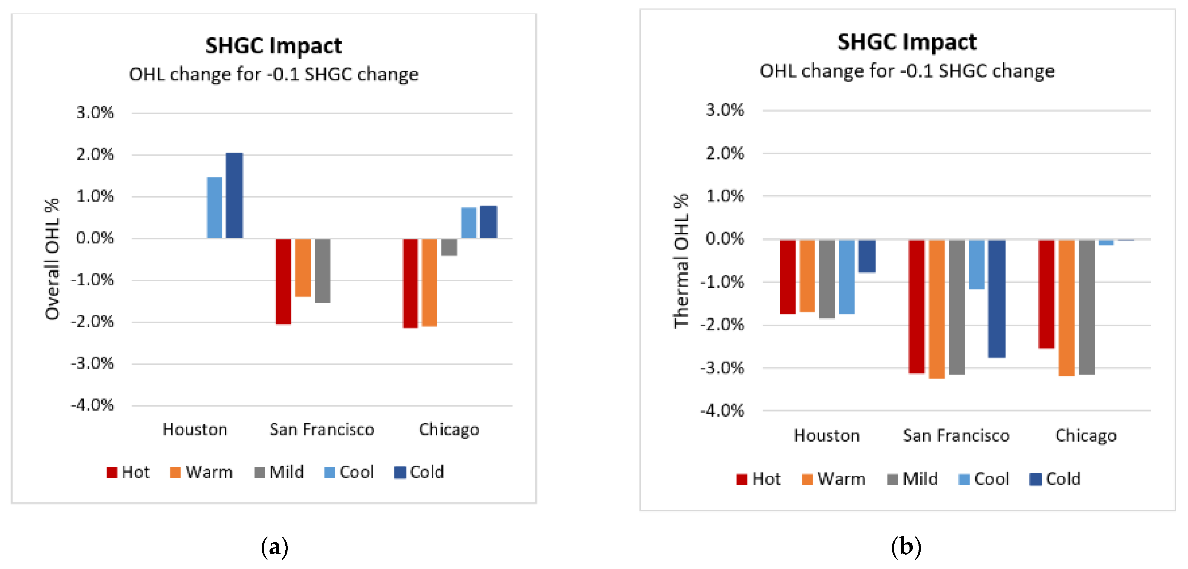
• Decreasing SHGC by 0.1 lowers thermal OHL by 1.8 to 3.3% in hot and warm weather weeks.
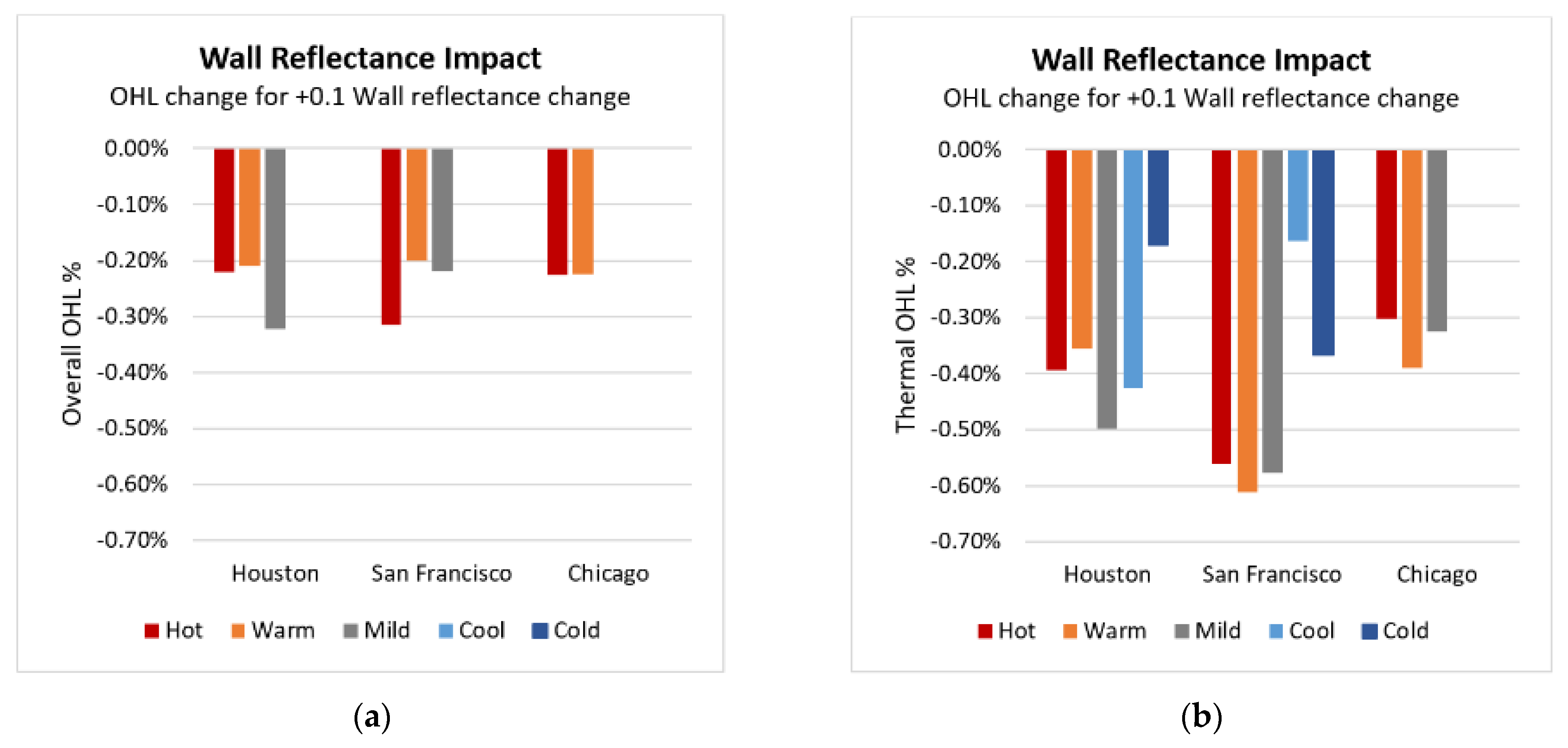
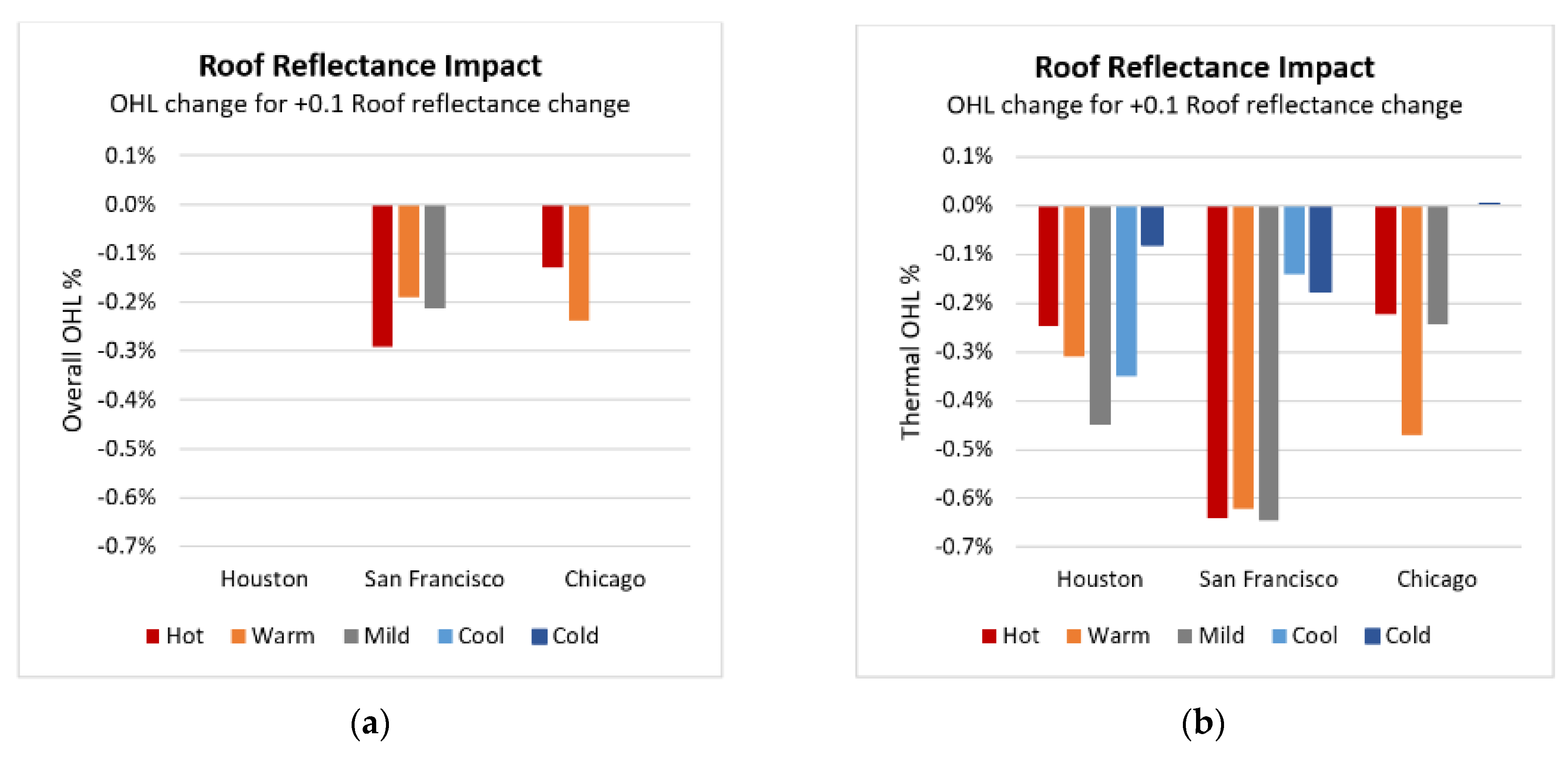
• Increasing wall reflectance and roof reflectance have approximately equivalent impacts on thermal OHL and have minimal if any impact on overall OHL.
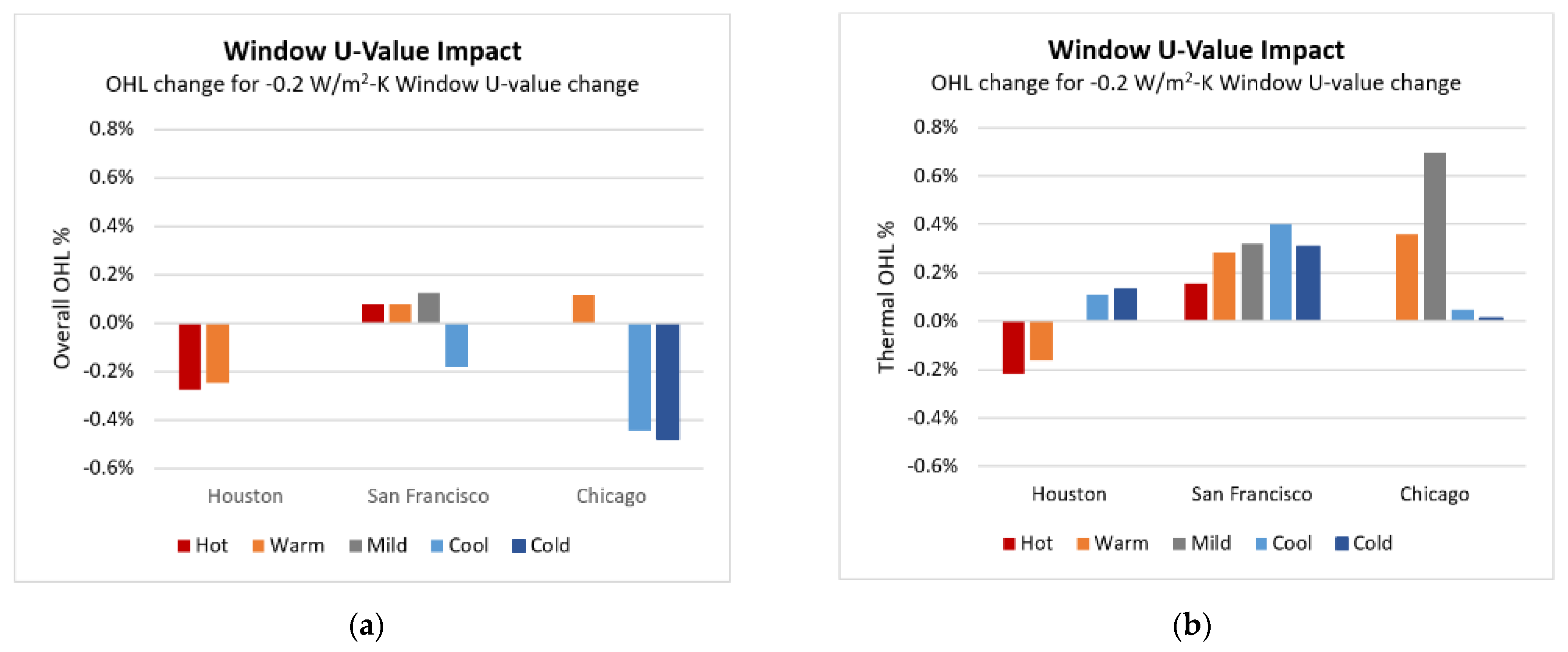
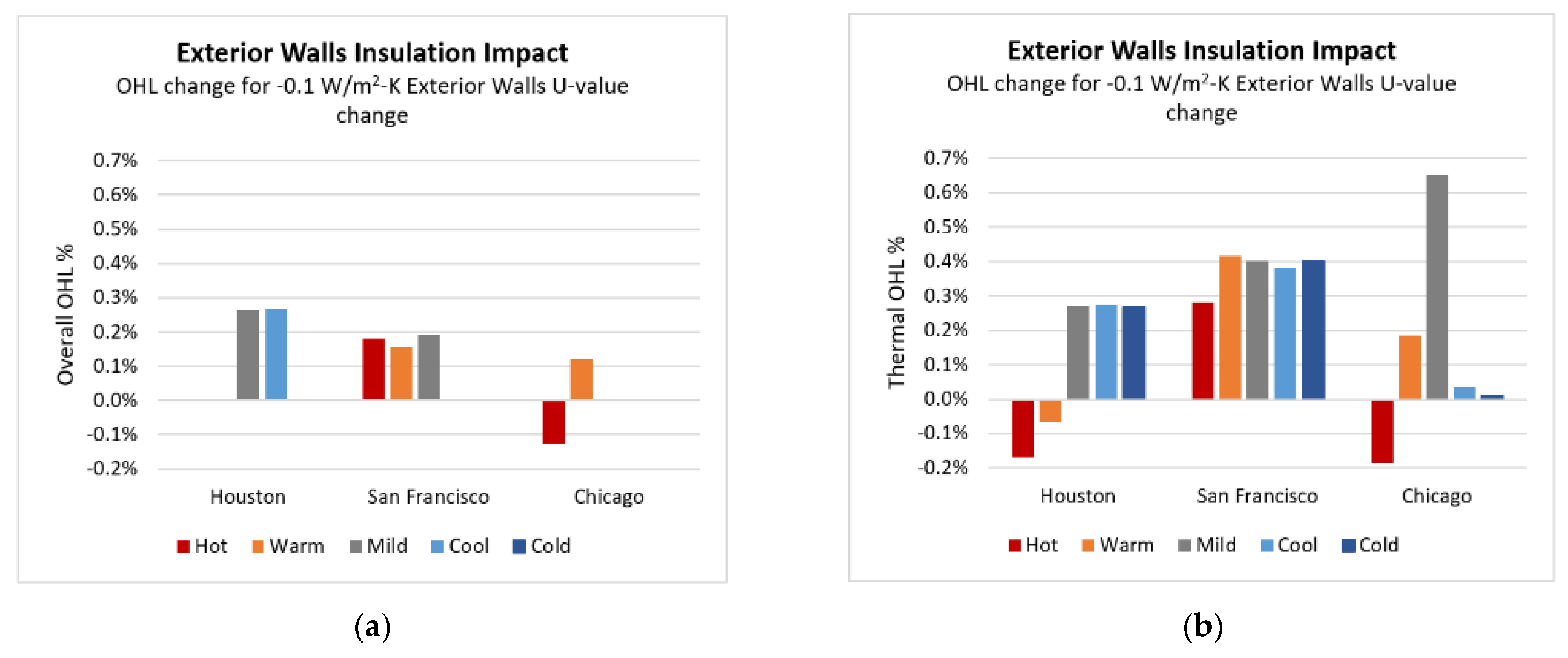
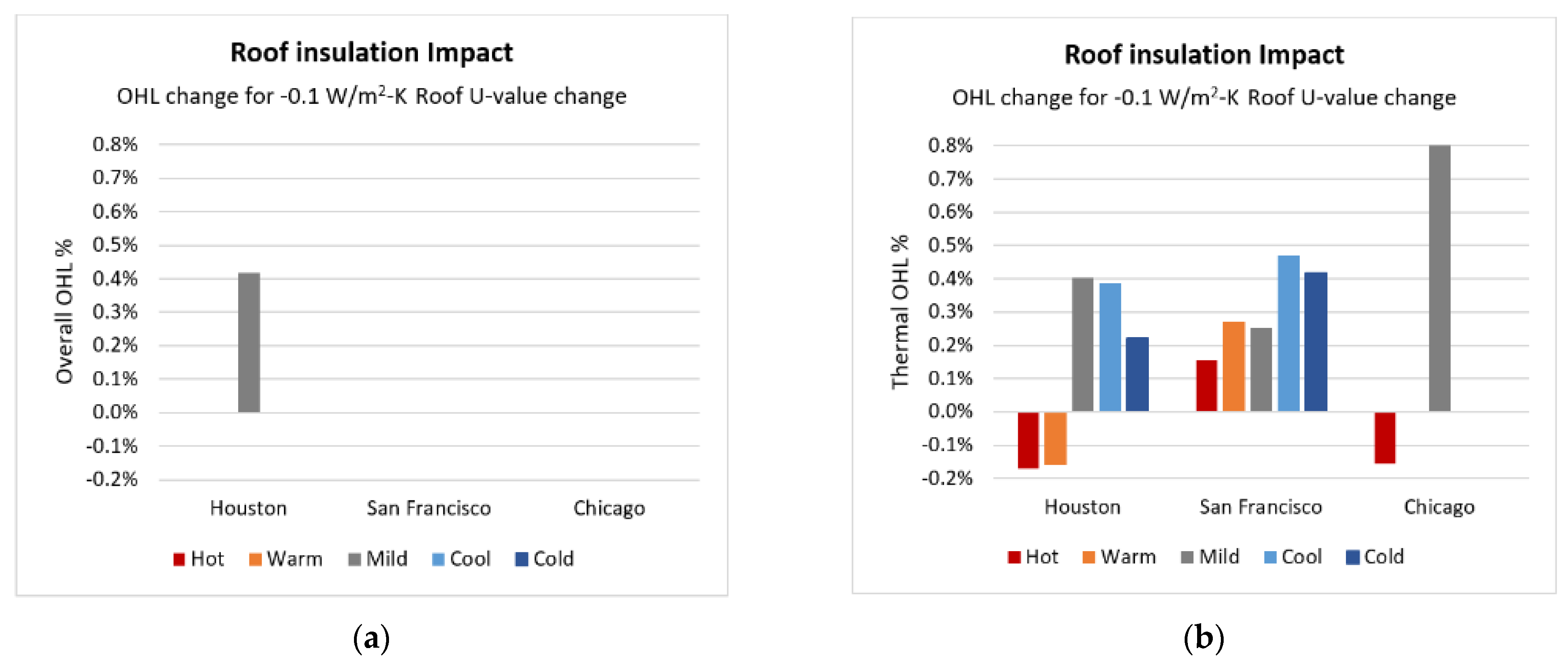
• Interestingly, reducing the U-value (i.e., increasing the insulation) of windows, walls, and roofs increases thermal OHL in cooler weather weeks-possibly because of the reduced ability to dissipate internal and solar gains when outdoor temperatures are lower.
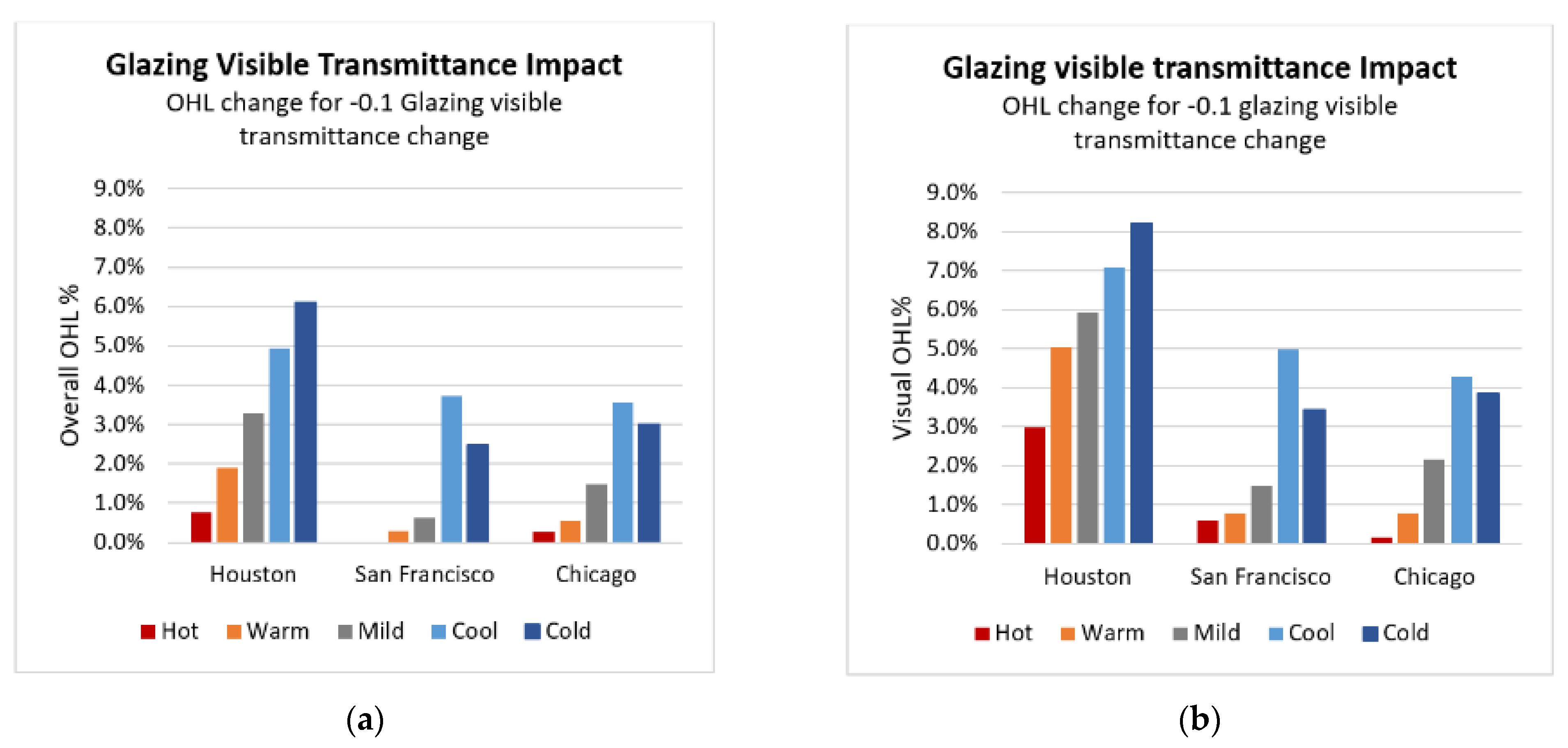
• As expected, a 0.1 decrease in visible transmittance significantly impacts visual OHL and overall OHL, with increasing impacts in cool and cold weeks (i.e., fall and winter).
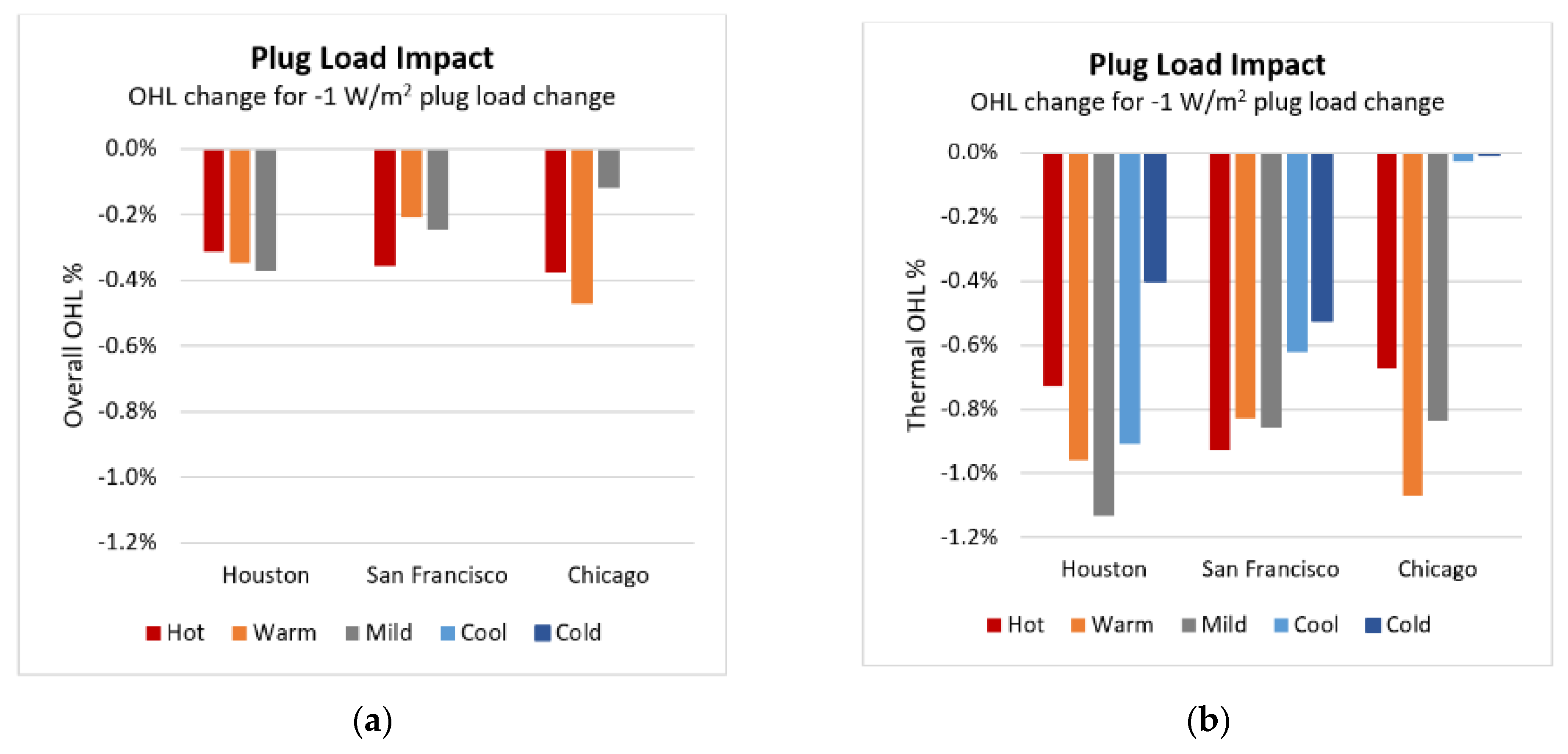
• Lowering plug loads by 11 W/sq.m (approximately 10% of typical office plug load values) reduces overall OHL by around 0.3–0.5% in hot and warm weeks.
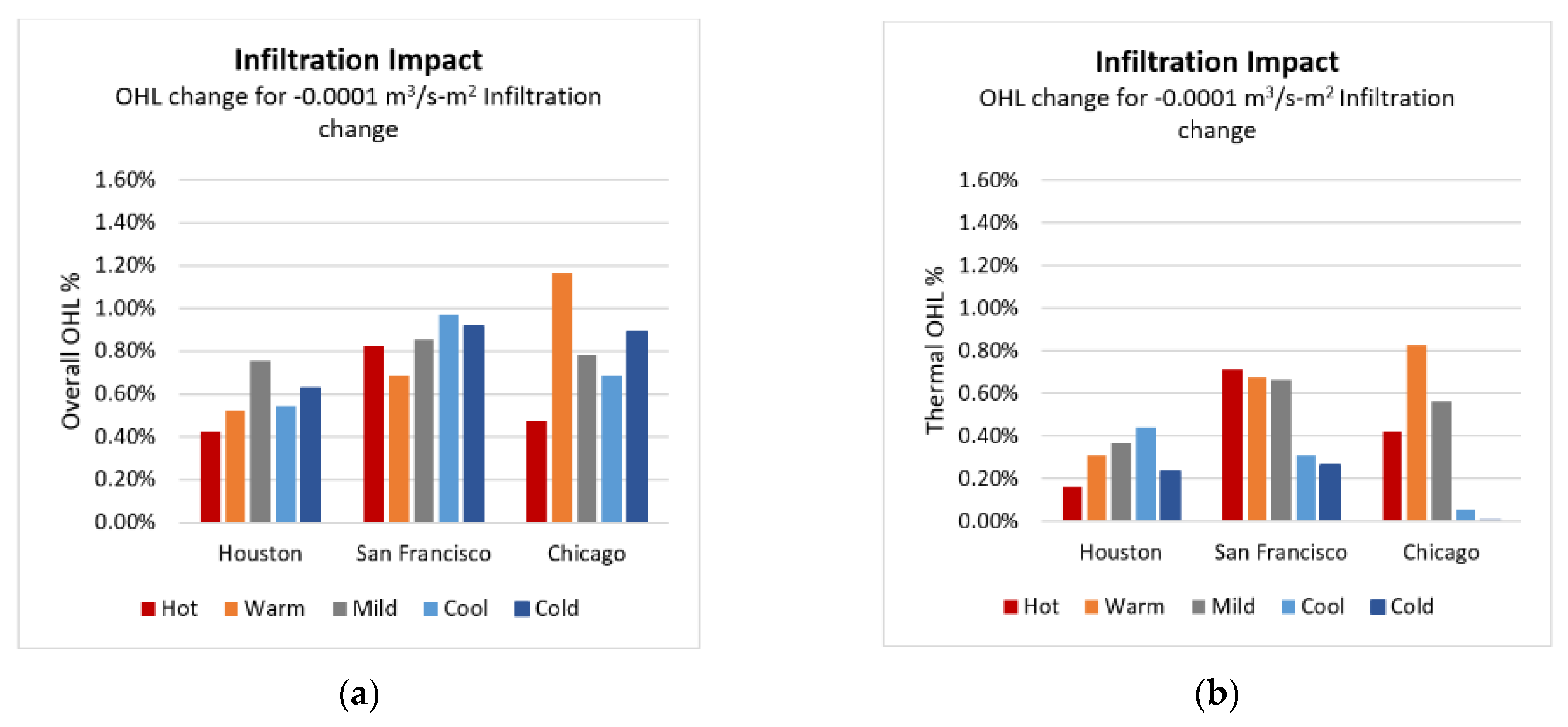
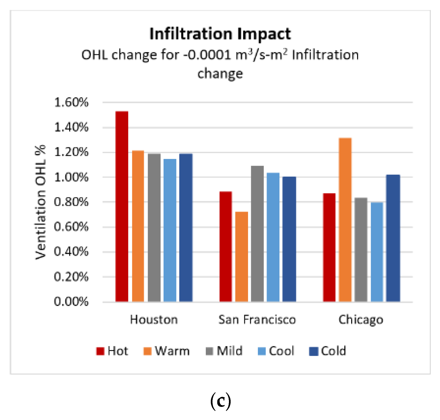
• Infiltration impacts appear to be minimal.
• Overall, it appears the most impactful parameters are WWR, SHGC, and visible transmittance. In particular, WWR and visible transmittance significantly impact daylight availability, which in turn significantly impacts visual OHL. In the case of thermal OHL, SHGC is more impactful than wall and roof insulation, suggesting that indoor thermal conditions appear to be more influenced by solar load than the outdoor temperature.

The model fit for most of the metrics and weather weeks were generally good, with a few exceptions (see again Appendix A Table A1, Table A2, Table A3 and Table A4). The adjusted R² varies from 0.59 to 0.96 for thermal OHL, 0.43–0.94 for visual OHL, 0.86 to 0.97 for ventilation OHL, and 0.45–0.93 for overall OHL.

The results show significant differences between the different OHL metrics. This also explains why overall OHL does not always offer intuitive or self-explanatory results. This suggests that it is important for stakeholders to evaluate metrics based on their priorities. For example, some owners may primarily be interested in reducing thermal OHL, on the premise that in a power outage, they can use some level of battery-powered lighting or consolidate building activities in daylit spaces.

A key limitation of these results is that geometry (shape and surface to volume ratio) was not a variable in the simulation dataset used for the analysis. Nevertheless, for buildings with similar rectangular geometry, the regression shows promise as a simple means to assess and screen for resilience, analogous to energy benchmarking. This is especially relevant for non-critical facilities where it may not be viable to conduct a rigorous energy resilience analysis using detailed building simulation.

6. Conclusions and Further Research

Energy resilience planning for the built environment has largely focused on maintaining key facility operations concerning human wellbeing and survival during natural disasters. Our study contributes to the growing body of research on building resilience in two ways:

• We propose “occupancy hours lost” (OHL) as a metric to capture the impact of a power outage. It can be calculated and aggregated at various levels of spatial and temporal resolution. It offers a relatively simple approach for evaluating the energy resilience of non-critical buildings, with a focus on supporting stakeholder priorities for business continuity during a power outage. Using parametric energy simulations, we illustrated how the metric varies due to different building characteristics, across different climate zones and seasons.
• We developed a simple predictive model for calculating OHL based on building characteristics, using the aforementioned simulation results. This would allow a first-order coarse evaluation of building energy resilience with a relatively low data burden.

There are several areas for further research:

• Our simulation analysis was limited to a particular building morphology and occupancy characteristics. This should be expanded to represent a range of morphologies, sizes, and occupancy characteristics in order to more robustly evaluate the potential of using simple regression models to predict OHL.
• Ultimately, the simulation-based datasets need to be complemented with empirical validation, which can be challenging due to the difficulty of emulating extreme events in real life. One potential approach may be to de-power a building, take measurements of indoor conditions, and compare these against the simulation results.
• Another area of further work is to analyze how the accuracy of the metric varies with the quantity and quality of data input. This is especially relevant to wider application in the building industry, where it is still challenging to get even basic information on building characteristics without significant effort. Metrics that provide moderate accuracy with low data burden are much more likely to be widely accepted and used than high fidelity metrics that have a high data burden.
• These metrics need to be field-validated by building industry stakeholders using them for actual business purposes.

Finally, we would reiterate that resilience is a very broad concept and no single metric can capture the diversity of use cases. Depending on the event scenario and stakeholder priorities, the energy resilience metric presented in this paper may need to be used in conjunction with other key resilience metrics, such as structural integrity in the case of an earthquake scenario. Other use cases may call for applying the metric to aggregations of buildings, so that resilience planners and policymakers can assess energy resilience at the community scale.

References

1. The White House. Presidential Policy Directive—Critical Infrastructure and Resilience. Presidential Policy Directive/PPD-21; Office of the Press Secretary: Washington, DC, USA, 2013. Available online: https://obamawhitehouse.archives.gov/the-press-office/2013/02/12/presidential-policy-directive-critical-infrastructure-security-and-resil (accessed on 23 February 2021).
2. Baniassadi, A.; Heusinger, J.; Sailor, D.J. Energy Efficiency vs Resiliency to Extreme Heat and Power Outages: The Role of Evolving Building Energy Codes. Build. Environ. 2018, 139, 86–94. [Google Scholar] [CrossRef]
3. McCunn, L.J.; Kim, A.; Feracor, J. Reflections on a Retrofit: Organizational Commitment, Perceived Productivity and Controllability in a Building Lighting Project in the United States. Energy Res. Soc. Sci. 2018, 38, 154–164. [Google Scholar] [CrossRef]
4. Mills, E. The Greening of Insurance. Science 2012, 338, 1424–1425. [Google Scholar] [CrossRef] [PubMed]
5. White, A.R.; Beach, M.S. A Case Study of Hurricane Katrina and Sandy Claims; Construction Law; DRI: Houston, TX, USA, 2017. [Google Scholar]
6. Bobotek, J.P.; Gillon, P.M.; Greeves, G.J.; Morgan, V.E. Critical Insurance Coverage Issues Emerging in the Wake of Sandy; Pillsbury Insights; Pillsbury Winthrop Shaw Pittman LLP: New York, NY, USA, 2013. [Google Scholar]
7. Roostaie, S.; Nawari, N.; Kibert, C.J. Sustainability and Resilience: A Review of Definitions, Relationships, and Their Integration into a Combined Building Assessment Framework. Build. Environ. 2019, 154, 132–144. [Google Scholar] [CrossRef]
8. O’Brien, W.; Tahmasebi, F.; Andersen, R.K.; Azar, E.; Barthelmes, V.; Belafi, Z.D.; Berger, C.; Chen, D.; De Simone, M.; d’Oca, S.; et al. An International Review of Occupant-Related Aspects of Building Energy Codes and Standards. Build. Environ. 2020, 179, 106906. [Google Scholar] [CrossRef]
9. Wilson, A. Passive Survivability: Keeping Occupants Safe in an Age of Disruptions. In Proceedings of the Comfort at the Extremes Conference, Dubai, United Arab Emirates, 20 June 2019. [Google Scholar]
10. Cutter, S.L.; Barnes, L.; Berry, M.; Burton, C.; Evans, E.; Tate, E.; Webb, J. A Place-Based Model for Understanding Community Resilience to Natural Disasters. Glob. Environ. Chang. 2008, 18, 598–606. [Google Scholar] [CrossRef]
11. Cutter, S.L.; Burton, C.G.; Emrich, C.T. Disaster Resilience Indicators for Benchmarking Baseline Conditions. J. Homel. Secur. Emerg. Manag. 2010, 7, 51. [Google Scholar] [CrossRef]
12. Carlson, J.L.; Haffenden, R.A.; Bassett, G.W.; Buehring, W.A.; Collins III, M.J.; Folga, S.M.; Petit, F.D.; Phillips, J.A.; Verner, D.R.; Whitfield, R.G. Resilience: Theory and Application; Argonne National Lab.(ANL): Argonne, IL, USA, 2012. [Google Scholar]
13. Anderson, K.; Laws, N.; Marr, S.; Lisell, L.; Jimenez, T.; Case, T.; Li, X.; Lohmann, D.; Cutler, D. Quantifying and Monetizing Renewable Energy Resiliency. Sustainability 2018, 10, 933. [Google Scholar] [CrossRef] [Green Version]
14. Roege, P.E.; Collier, Z.A.; Mancillas, J.; McDonagh, J.A.; Linkov, I. Metrics for Energy Resilience. Energy Policy 2014, 72, 249–256. [Google Scholar] [CrossRef]
15. Petit, F.D.P.; Bassett, G.W.; Black, R.; Buehring, W.A.; Collins, M.J.; Dickinson, D.C.; Fisher, R.E.; Haffenden, R.A.; Huttenga, A.A.; Klett, M.S. Resilience Measurement Index: An Indicator of Critical Infrastructure Resilience; Argonne National Lab.(ANL): Argonne, IL, USA, 2013. [Google Scholar]
16. Bie, Z.; Lin, Y.; Li, G.; Li, F. Battling the Extreme: A Study on the Power System Resilience. Proc. IEEE 2017, 105, 1253–1266. [Google Scholar] [CrossRef]
17. Fisher, R.E.; Bassett, G.W.; Buehring, W.A.; Collins, M.J.; Dickinson, D.C.; Eaton, L.K.; Haffenden, R.A.; Hussar, N.E.; Klett, M.S.; Lawlor, M.A. Constructing a Resilience Index for the Enhanced Critical Infrastructure Protection Program; Argonne National Lab.(ANL): Argonne, IL, USA, 2010. [Google Scholar]
18. Hasik, V.; Chhabra, J.P.S.; Warn, G.P.; Bilec, M.M. Investigation of the Sustainability and Resilience Characteristics of Buildings Including Existing and Potential Assessment Metrics. Am. Soc. Civ. Eng. 2017, 2017, 1019–1033. [Google Scholar] [CrossRef]
19. U.S. Green Building Council. LEED Resilient Design Pilot Credits; U.S. Green Building Council: Washington, DC, USA, 2019. [Google Scholar]
20. USGBC. RELi 2.0 Rating Guidelines for Resilient Design+ Construction; USGBC: Washington, DC, USA, 2018. [Google Scholar]
21. Mayes, R.L.; Reis, E. Community Resilience and the US Resiliency Council’s Building Rating System. In Proceedings of the NZSEE Conference 2017, Wellington, New Zealand, 27–29 April 2017. [Google Scholar]
22. Marjaba, G.E.; Chidiac, S.E. Sustainability and Resiliency Metrics for Buildings—Critical Review. Build. Environ. 2016, 101, 116–125. [Google Scholar] [CrossRef]
23. Burroughs, S. Development of a Tool for Assessing Commercial Building Resilience. Procedia Eng. 2017, 180, 1034–1043. [Google Scholar] [CrossRef]
24. Ozkan, A.; Kesik, T.; Yilmaz, A.Z.; O’Brien, W. Development and Visualization of Time-Based Building Energy Performance Metrics. Build. Res. Inf. 2019, 47, 493–517. [Google Scholar] [CrossRef]
25. Ko, W.H.; Schiavon, S.; Brager, G.; Levitt, B. Ventilation, Thermal and Luminous Autonomy Metrics for an Integrated Design Process. Build. Environ. 2018, 145, 153–165. [Google Scholar] [CrossRef] [Green Version]
26. Ayyagari, S.; Gartman, M. A Framework for Considering Resilience in Building Envelope Design and Construction; Rocky Mountain Institute: Basalt, CO, USA, 2020. [Google Scholar]
27. Dyson, M.; Li, B. Reimagining Grid Resilience; Rocky Mountain Institute: Basalt, CO, USA, 2020; Available online: http://www.rmi.org/insight/reimagining-grid-resilience (accessed on 3 March 2021).
28. GridOptimal Metrics Offer Guidance on Optimizing Building-Grid Interaction. Available online: https://newbuildings.org/gridoptimal-metrics-offer-guidance-on-optimizing-building-grid-interaction/ (accessed on 4 December 2020).
29. Anderson, K.; Burman, K.; Simpkins, T.; Helson, E.; Lisell, L. New York Solar Smart DG Hub-Resilient Solar Project: Economic and Resiliency Impact of PV and Storage on New York Critical Infrastructure; Technical Report NREL/TP-7A40-66617; National Renewable Energy Lab.(NREL): Golden, CO, USA, 2016.
30. Charani Shandiz, S.; Foliente, G.; Rismanchi, B.; Wachtel, A.; Jeffers, R.F. Resilience Framework and Metrics for Energy Master Planning of Communities. Energy 2020, 203, 117856. [Google Scholar] [CrossRef]
31. Sun, K.; Specian, M.; Hong, T. Nexus of Thermal Resilience and Energy Efficiency in Buildings: A Case Study of a Nursing Home. Build. Environ. 2020, 177, 106842. [Google Scholar] [CrossRef]
32. Liu, S.; Kwok, Y.T.; Lau, K.K.-L.; Ouyang, W.; Ng, E. Effectiveness of Passive Design Strategies in Responding to Future Climate Change for Residential Buildings in Hot and Humid Hong Kong. Energy Build. 2020, 228, 110469. [Google Scholar] [CrossRef]
33. ANSI/ASHRAE. Standard 55-2017 Thermal Environmental Conditions for Human Occupancy; ASHRAE: Atlanta, GA, USA, 2017. [Google Scholar]
34. Standard 62.1-2019—American Society of Heating, Refrigerating and Air-Conditioning Engineers. Available online: https://ashrae.iwrapper.com/ASHRAE_PREVIEW_ONLY_STANDARDS/STD_62.1_2019 (accessed on 4 December 2020).
35. Standard 62.2-2019—American Society of Heating, Refrigerating and Air-Conditioning Engineers. Available online: https://ashrae.iwrapper.com/ASHRAE_PREVIEW_ONLY_STANDARDS/STD_62.2_2019 (accessed on 4 December 2020).
36. ASHRAE. ANSI/ASHRAE/IES Standard 90.1 Energy Standard for Buildings Except Low-Rise Residential Buildings; ASHRAE: Atlanta, GA, USA, 2019. [Google Scholar]
37. Sanchez, L.; Mathew, P.; Lee, S.H.; Walter, T. Developing and Evaluating a Metric for Office Building Energy Resilience during a Power Outage. In Proceedings of the ACEEE 2020 Summer Study on Energy Efficiency in Buildings, Virtual Event, Pacific Grove, CA, USA, 17–21 August 2020. [Google Scholar]
38. Zhang, S.; Lin, Z. Standard Effective Temperature Based Adaptive-Rational Thermal Comfort Model. Appl. Energy 2020, 264, 114723. [Google Scholar] [CrossRef]
39. Niemann, P.; Schmitz, G. Impacts of Occupancy on Energy Demand and Thermal Comfort for a Large-Sized Administration Building. Build. Environ. 2020, 182, 107027. [Google Scholar] [CrossRef]
40. Criteria for a Recommended Standard: Occupational Exposure to Carbon Dioxide; National Institute for Occupational Safety and Health: Washington, DC, USA, 1976.
41. Ludwig, H.R.; Cairelli, S.G.; Whalen, J.J. Documentation for Immediately Dangerous to Life or Health Concentrations (IDLHs); National Institute for Occupational Safety and Health: Cincinnati, OH, USA, 1994.
42. Goel, S.; Athalye, R.A.; Wang, W.; Zhang, J.; Rosenberg, M.I.; Xie, Y.; Hart, P.R.; Mendon, V.V. Enhancements to ASHRAE Standard 90.1 Prototype Building Models; Pacific Northwest National Lab.(PNNL): Richland, WA, USA, 2014.
43. Im, P.; New, J.R.; Bae, Y. Updated OpenStudio Small and Medium Office Prototype Models. In Proceedings of the 16th IBPSA International Conference & Exhibition on Building Simulation, Rome, Italy, 2–4 September 2019. [Google Scholar]
44. Updated Small/Medium/Large Office Models with Detailed Space Types. Available online: https://github.com/NREL/openstudio-standards/pull/562 (accessed on 4 December 2020).
45. Commercial Prototype Building Models. Available online: https://www.energycodes.gov/development/commercial/prototype_models (accessed on 14 September 2020).
46. Commercial Reference Buildings. Available online: https://www.energy.gov/eere/buildings/commercial-reference-buildings (accessed on 14 September 2020).
Figure 1. Floor plan and geometry of the DOE medium office 90.1-2007 prototype model with detailed zoning.
Buildings 11 00096 g001
Figure 2. Thermal OHL for Houston (a), San Francisco (b), Chicago (c).
Buildings 11 00096 g002
Figure 3. Visual OHL for Houston (a), San Francisco (b), Chicago (c).
Buildings 11 00096 g003
Figure 4. Ventilation OHL for Houston (a), San Francisco (b), Chicago (c).
Buildings 11 00096 g004
Figure 5. Overall OHL for Houston (a), San Francisco (b), Chicago (c).
Buildings 11 00096 g005
Figure 6. Thermal OHL in different zones for a hot weather week in Houston.
Buildings 11 00096 g006
Figure 7. Impact of a 0.1 decrease in window-to-wall ratio (WWR) on overall (a), thermal (b), and visual (c) OHL.
Buildings 11 00096 g007
Figure 8. Impact of a 0.1 decrease in SHGC on overall (a) and thermal (b) OHL.
Buildings 11 00096 g008
Figure 9. Impact of a 0.2 W/m2-K decrease in window U-value on overall (a) and thermal (b) OHL.
Buildings 11 00096 g009
Figure 10. Impact of a 0.1 W/m2-K decrease in exterior wall U-value on overall (a) and thermal (b) OHL.
Buildings 11 00096 g010
Figure 11. Impact of a 0.1 W/m2-K decrease in roof insulation U-value on overall (a) and thermal (b) OHL.
Buildings 11 00096 g011
Figure 12. Impact of a 0.1 increase in wall reflectance on overall (a) and thermal (b) OHL.
Buildings 11 00096 g012
Figure 13. Impact of a 0.1 increase in roof reflectance on overall (a) and thermal (b) OHL.
Buildings 11 00096 g013
Figure 14. Impact of a 1 W/sq.m decrease in plug loads on overall (a) and thermal (b) OHL.
Buildings 11 00096 g014
Figure 15. Impact of a 0.1 decrease in glazing visible transmittance on overall (a) and visual (b) OHL.
Buildings 11 00096 g015
Figure 16. Impact of a 0.0001 m3/s-m2 decrease in infiltration rate on overall (a), thermal (b) and ventilation (c) OHL.
Buildings 11 00096 g016aBuildings 11 00096 g016b