
Mechanical Performance Prediction for Sustainable High-Strength Concrete Using Bio-Inspired Neural Network

 ,
,
Abstract
:1. Introduction
2. Dataset
3. Methodology
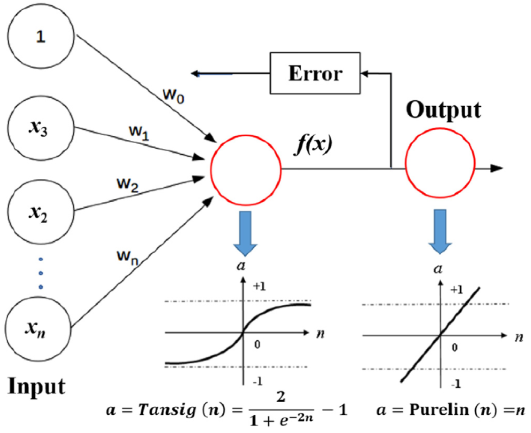
3.1. BPNN
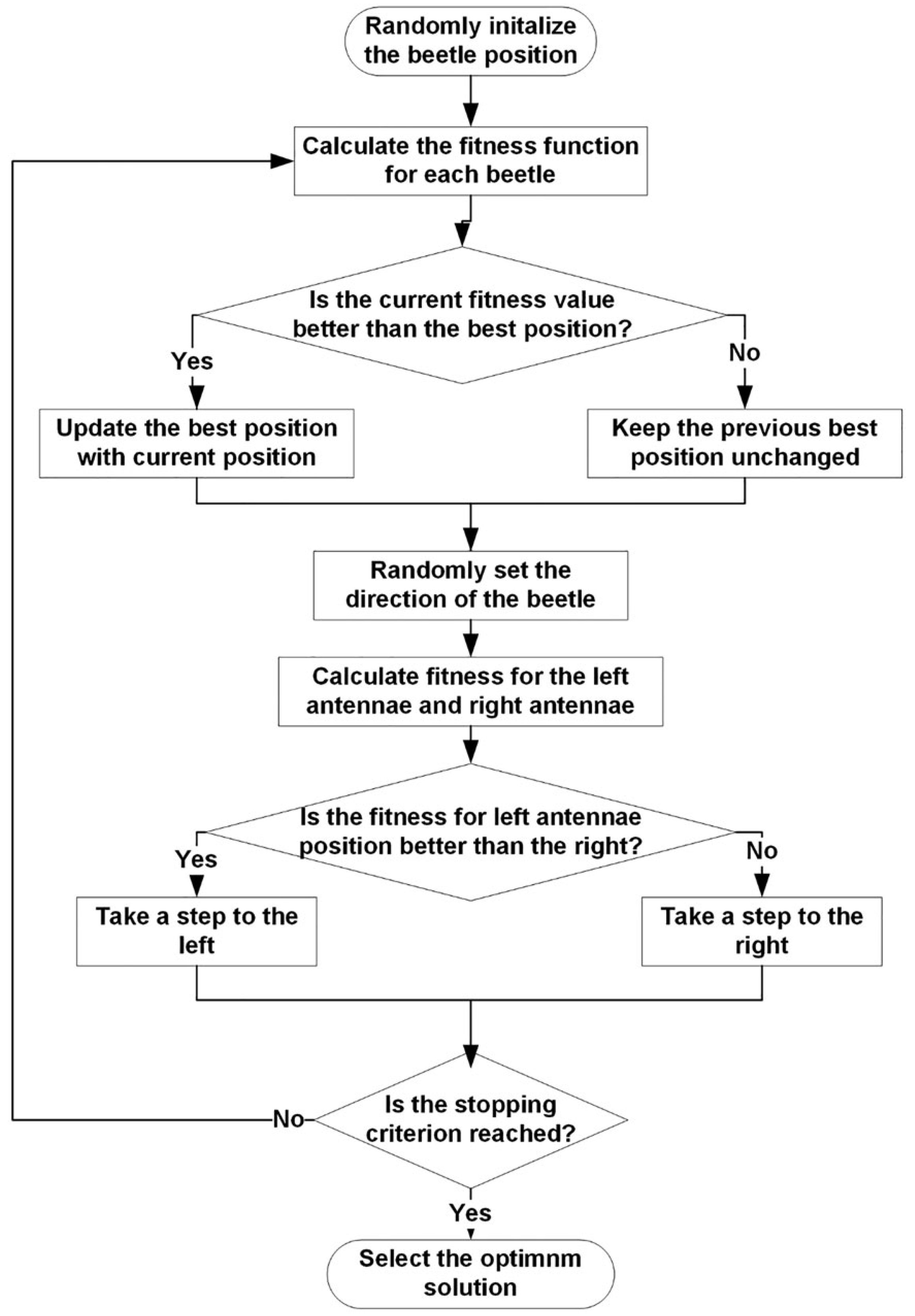
3.2. BAS
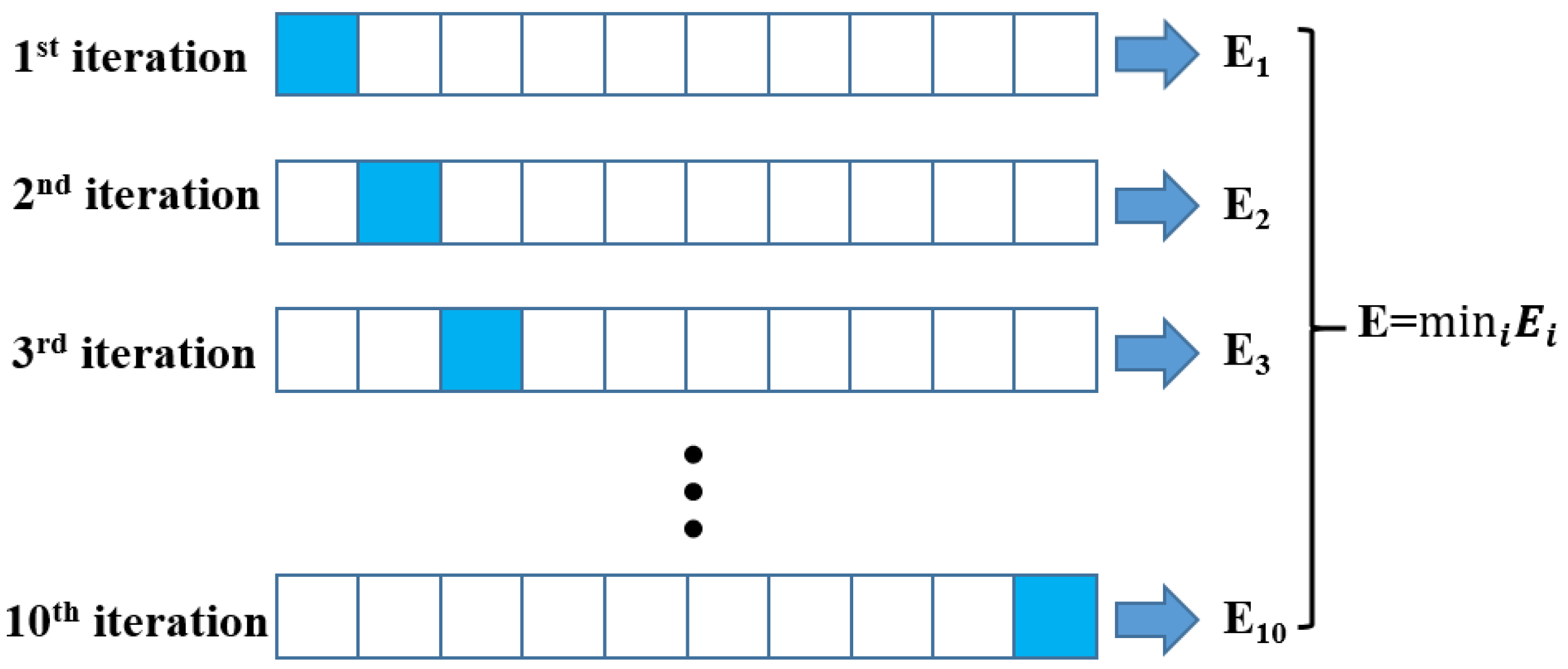
3.3. Performance Evaluation
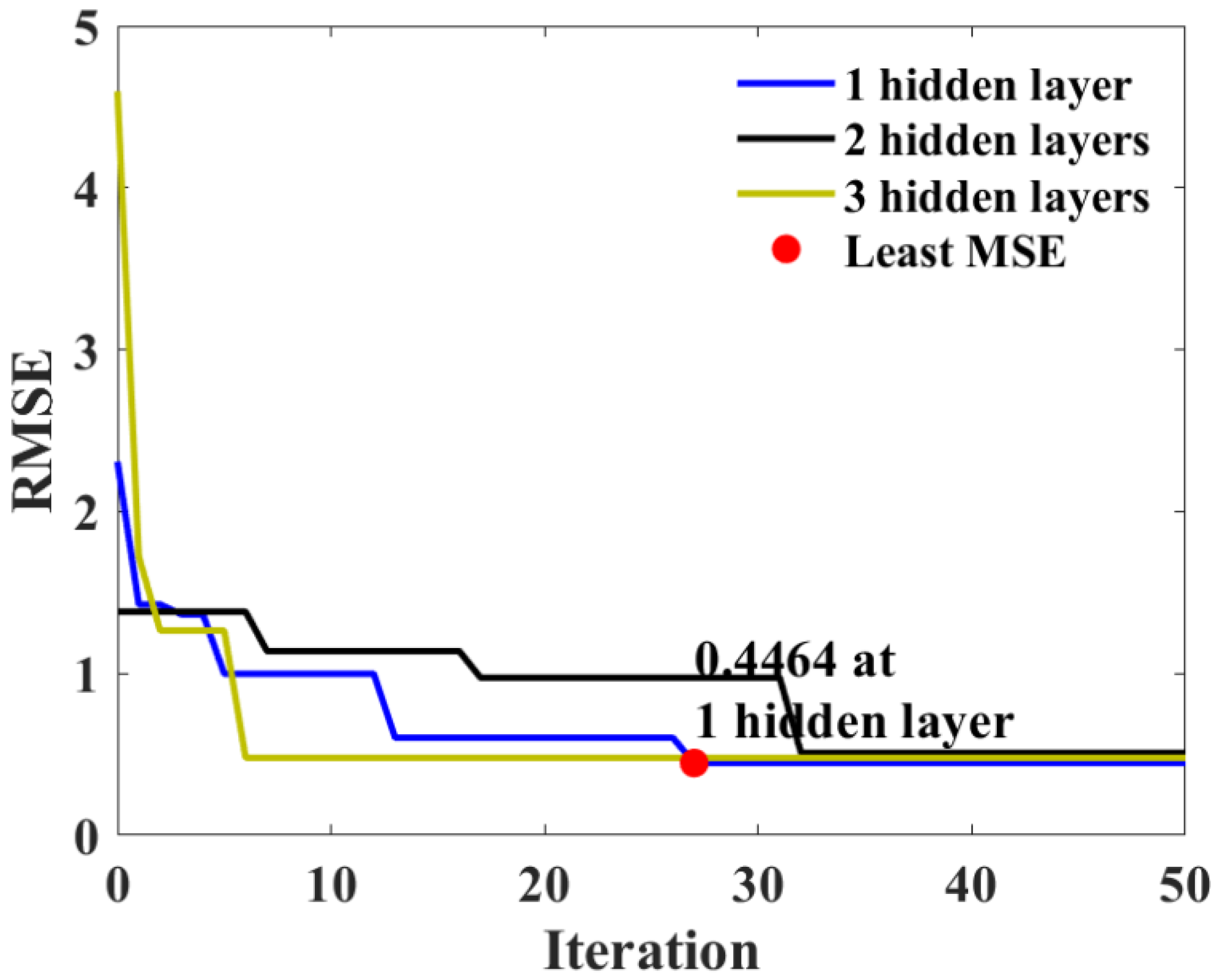
3.4. Determination of Architecture of BPNN
4. Results and Discussion
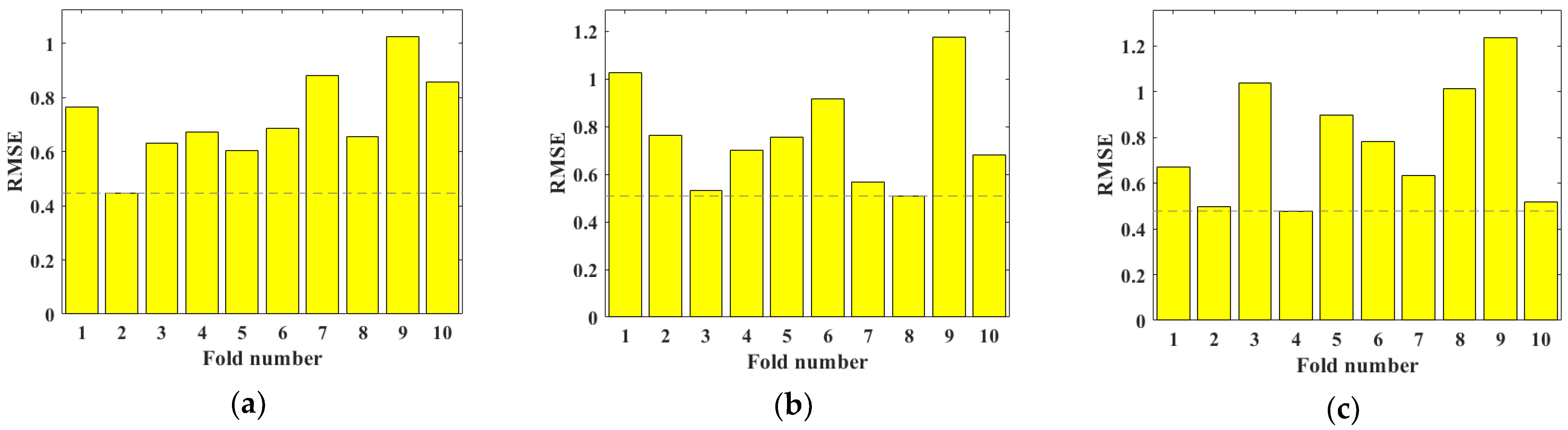
4.1. Results of Hyperparameter Tuning
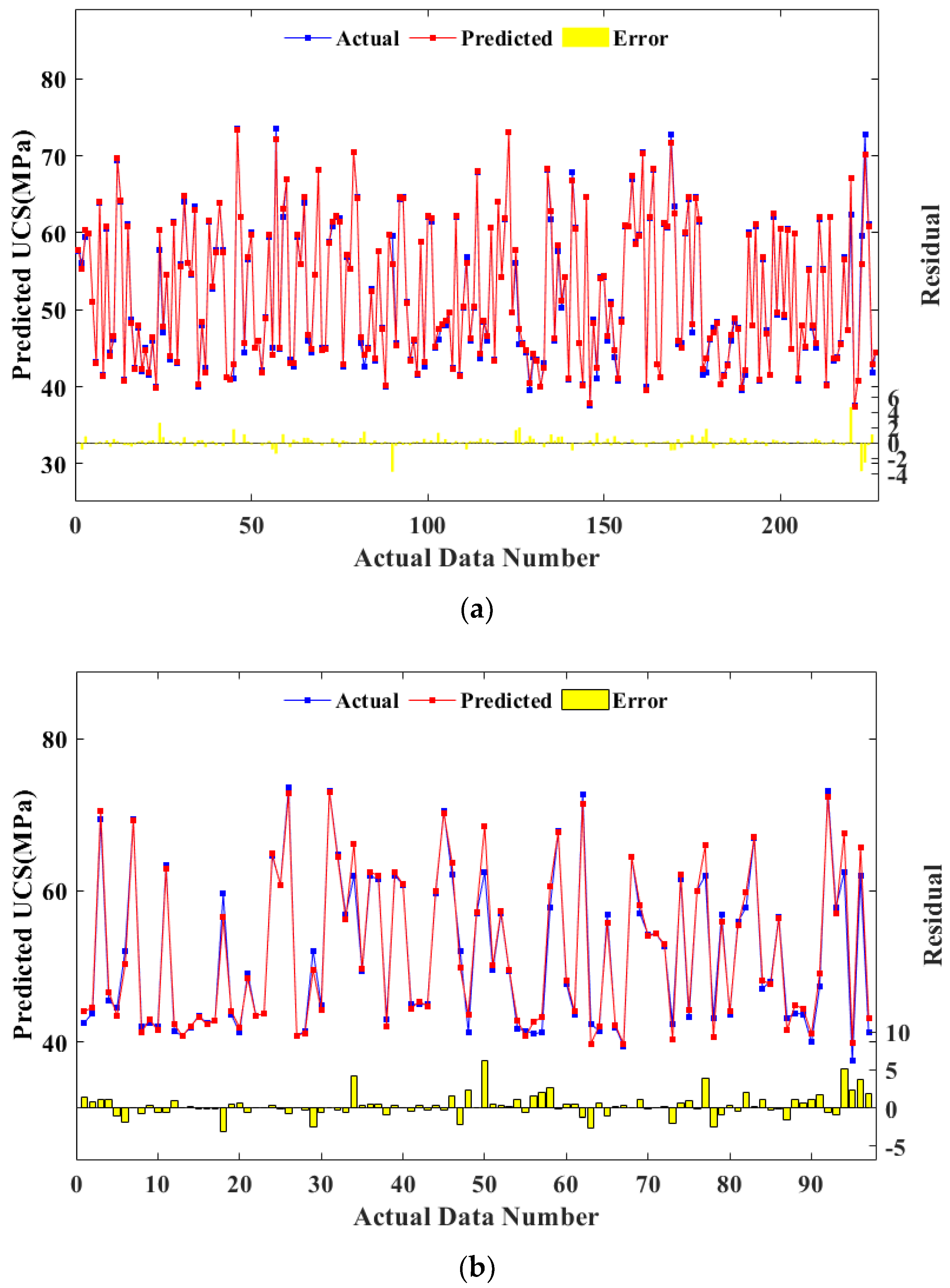
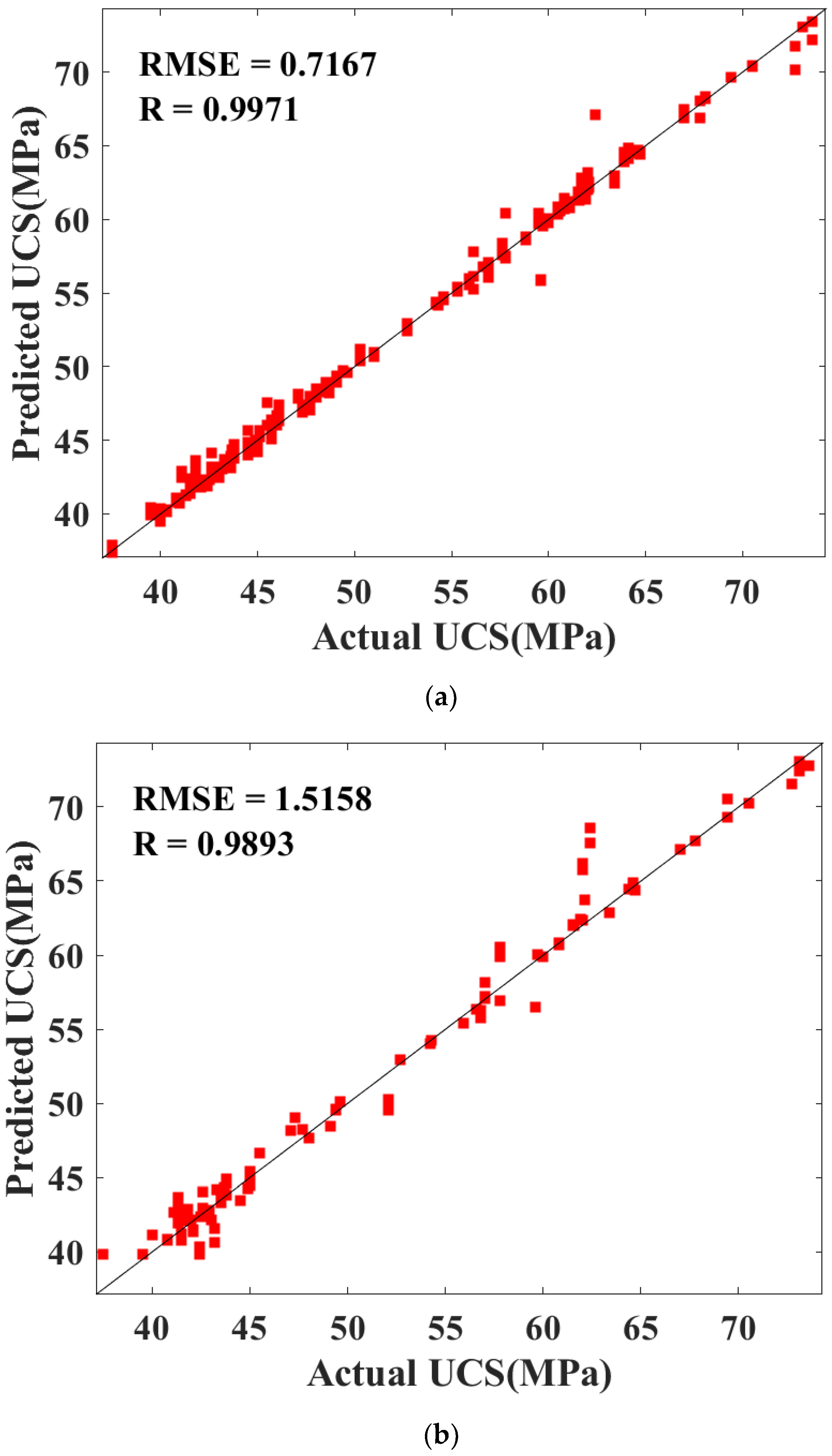
4.2. Performance of the BAS-BPNN Model
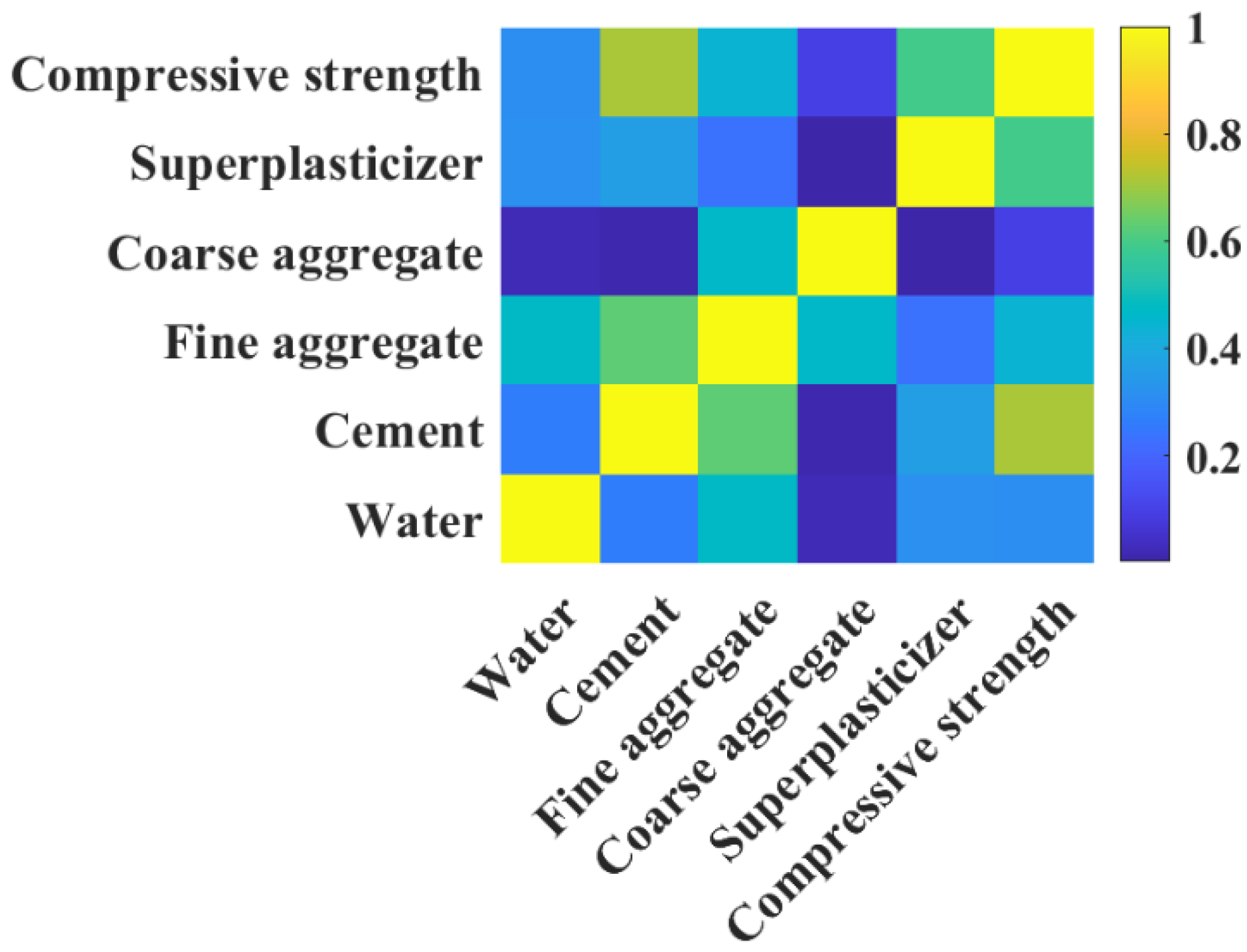
4.3. Variable Importance
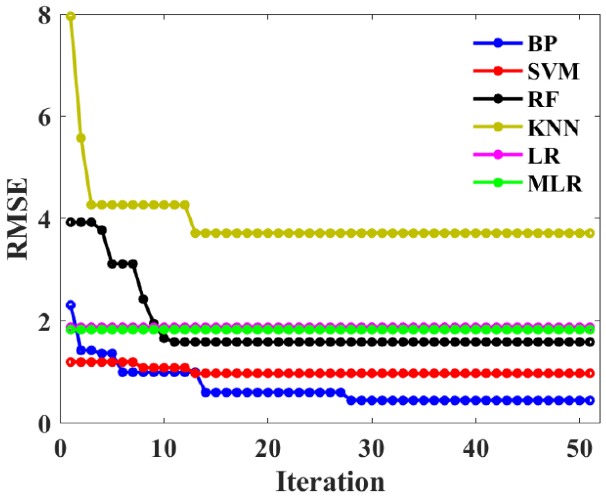
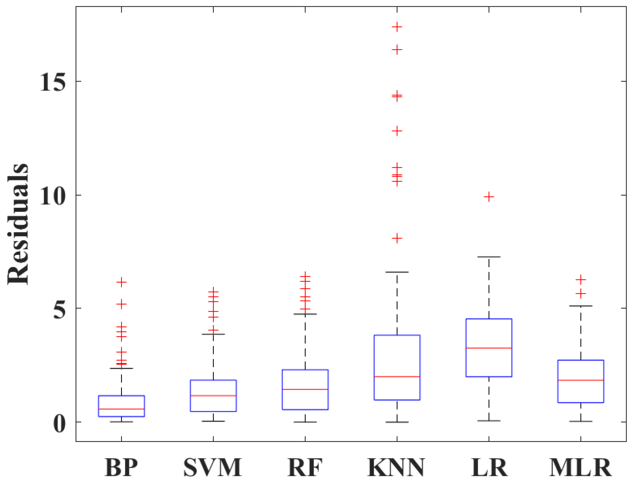
4.4. Comparison of the BAS-BPNN Model with Other ML Models
5. Conclusions
Author Contributions
Funding
Data Availability Statement
Conflicts of Interest
Appendix A

| ID | Water (kg/m3) | OPC (kg/m3) | FA (kg/m3) | CA (kg/m3) | SP (kg/m3) | UCS (MPa) |
|---|---|---|---|---|---|---|
| 1 | 160 | 533 | 805 | 845 | 1 | 73.6 |
| 2 | 160 | 533 | 805 | 845 | 1.5 | 73.6 |
| 3 | 160 | 533 | 805 | 845 | 2 | 73.6 |
| 4 | 160 | 480 | 786 | 845 | 1 | 73.1 |
| 5 | 160 | 480 | 786 | 845 | 1.5 | 73.1 |
| 6 | 160 | 480 | 786 | 845 | 2 | 73.1 |
| 7 | 160 | 427 | 767 | 845 | 1 | 72.7 |
| 8 | 160 | 427 | 767 | 845 | 1.5 | 72.7 |
| 9 | 160 | 427 | 767 | 845 | 2 | 72.7 |
| 10 | 160 | 533 | 753 | 898 | 1 | 69.4 |
| 11 | 160 | 533 | 753 | 898 | 1.5 | 69.4 |
| 12 | 160 | 533 | 753 | 898 | 2 | 69.4 |
| 13 | 160 | 480 | 734 | 898 | 1 | 70.5 |
| 14 | 160 | 480 | 734 | 898 | 1.5 | 70.5 |
| 15 | 160 | 480 | 734 | 898 | 2 | 70.5 |
| 16 | 160 | 427 | 715 | 898 | 1 | 68.1 |
| 17 | 160 | 427 | 715 | 898 | 1.5 | 68.1 |
| 18 | 160 | 427 | 715 | 898 | 2 | 68.1 |
| 19 | 160 | 533 | 701 | 950 | 1 | 67.8 |
| 20 | 160 | 533 | 701 | 950 | 1.5 | 67.8 |
| 21 | 160 | 533 | 701 | 950 | 2 | 67.8 |
| 22 | 160 | 480 | 682 | 950 | 1 | 67 |
| 23 | 160 | 480 | 682 | 950 | 1.5 | 67 |
| 24 | 160 | 480 | 682 | 950 | 2 | 67 |
| 25 | 160 | 427 | 663 | 950 | 1 | 64.1 |
| 26 | 160 | 427 | 663 | 950 | 1.5 | 64.1 |
| 27 | 160 | 427 | 663 | 950 | 2 | 64.1 |
| 28 | 170 | 567 | 751 | 845 | 1 | 64.6 |
| 29 | 170 | 567 | 751 | 845 | 1.5 | 64.6 |
| 30 | 170 | 567 | 751 | 845 | 2 | 64.6 |
| 31 | 170 | 510 | 731 | 845 | 1 | 64.4 |
| 32 | 170 | 510 | 731 | 845 | 1.5 | 64.4 |
| 33 | 170 | 510 | 731 | 845 | 2 | 64.4 |
| 34 | 170 | 453 | 711 | 845 | 1 | 64.7 |
| 35 | 170 | 453 | 711 | 845 | 1.5 | 64.7 |
| 36 | 170 | 453 | 711 | 845 | 2 | 64.7 |
| 37 | 170 | 567 | 700 | 898 | 1 | 63.9 |
| 38 | 170 | 567 | 700 | 898 | 1.5 | 63.9 |
| 39 | 170 | 567 | 700 | 898 | 2 | 63.9 |
| 40 | 170 | 510 | 679 | 898 | 1 | 63.4 |
| 41 | 170 | 510 | 679 | 898 | 1.5 | 63.4 |
| 42 | 170 | 510 | 679 | 898 | 2 | 63.4 |
| 43 | 170 | 453 | 659 | 898 | 1 | 62 |
| 44 | 170 | 453 | 659 | 898 | 1.5 | 62 |
| 45 | 170 | 453 | 659 | 898 | 2 | 62 |
| 46 | 170 | 567 | 648 | 950 | 1 | 62.4 |
| 47 | 170 | 567 | 648 | 950 | 1.5 | 62.4 |
| 48 | 170 | 567 | 648 | 950 | 2 | 62.4 |
| 49 | 170 | 510 | 628 | 950 | 1 | 61.7 |
| 50 | 170 | 510 | 628 | 950 | 1.5 | 61.7 |
| 51 | 170 | 510 | 628 | 950 | 2 | 61.7 |
| 52 | 170 | 453 | 608 | 950 | 1 | 61.9 |
| 53 | 170 | 453 | 608 | 950 | 1.5 | 61.9 |
| 54 | 170 | 453 | 608 | 950 | 2 | 61.9 |
| 55 | 180 | 600 | 698 | 845 | 0.75 | 59.5 |
| 56 | 180 | 600 | 698 | 845 | 1.25 | 59.5 |
| 57 | 180 | 600 | 698 | 845 | 1.75 | 59.5 |
| 58 | 180 | 540 | 677 | 845 | 0.75 | 61.1 |
| 59 | 180 | 540 | 677 | 845 | 1.25 | 61.1 |
| 60 | 180 | 540 | 677 | 845 | 1.75 | 61.1 |
| 61 | 180 | 480 | 655 | 845 | 0.75 | 60.8 |
| 62 | 180 | 480 | 655 | 845 | 1.25 | 60.8 |
| 63 | 180 | 480 | 655 | 845 | 1.75 | 60.8 |
| 64 | 180 | 600 | 646 | 898 | 0.75 | 60.5 |
| 65 | 180 | 600 | 646 | 898 | 1.25 | 60.5 |
| 66 | 180 | 600 | 646 | 898 | 1.75 | 60.5 |
| 67 | 180 | 540 | 625 | 898 | 0.75 | 59.9 |
| 68 | 180 | 540 | 625 | 898 | 1.25 | 59.9 |
| 69 | 180 | 540 | 625 | 898 | 1.75 | 59.9 |
| 70 | 180 | 480 | 604 | 898 | 0.75 | 57 |
| 71 | 180 | 480 | 604 | 898 | 1.25 | 57 |
| 72 | 180 | 480 | 604 | 898 | 1.75 | 57 |
| 73 | 180 | 600 | 594 | 950 | 0.75 | 59.7 |
| 74 | 180 | 600 | 594 | 950 | 1.25 | 59.7 |
| 75 | 180 | 600 | 594 | 950 | 1.75 | 59.7 |
| 76 | 180 | 540 | 573 | 950 | 0.75 | 60 |
| 77 | 180 | 540 | 573 | 950 | 1.25 | 60 |
| 78 | 180 | 540 | 573 | 950 | 1.75 | 60 |
| 79 | 180 | 480 | 552 | 950 | 0.75 | 59.6 |
| 80 | 180 | 480 | 552 | 950 | 1.25 | 59.6 |
| 81 | 180 | 480 | 552 | 950 | 1.75 | 59.6 |
| 82 | 160 | 457 | 867 | 845 | 0.75 | 62 |
| 83 | 160 | 457 | 867 | 845 | 1.25 | 62 |
| 84 | 160 | 457 | 867 | 845 | 1.75 | 62 |
| 85 | 160 | 411 | 851 | 845 | 0.75 | 62 |
| 86 | 160 | 411 | 851 | 845 | 1.25 | 62 |
| 87 | 160 | 411 | 851 | 845 | 1.75 | 62 |
| 88 | 160 | 366 | 835 | 845 | 0.75 | 60.6 |
| 89 | 160 | 366 | 835 | 845 | 1.25 | 60.6 |
| 90 | 160 | 366 | 835 | 845 | 1.75 | 60.6 |
| 91 | 160 | 457 | 816 | 898 | 0.75 | 62.1 |
| 92 | 160 | 457 | 816 | 898 | 1.25 | 62.1 |
| 93 | 160 | 457 | 816 | 898 | 1.75 | 62.1 |
| 94 | 160 | 411 | 799 | 898 | 0.75 | 61.5 |
| 95 | 160 | 411 | 799 | 898 | 1.25 | 61.5 |
| 96 | 160 | 411 | 799 | 898 | 1.75 | 61.5 |
| 97 | 160 | 366 | 783 | 898 | 0.75 | 57.8 |
| 98 | 160 | 366 | 783 | 898 | 1.25 | 57.8 |
| 99 | 160 | 366 | 783 | 898 | 1.75 | 57.8 |
| 100 | 160 | 457 | 764 | 950 | 0.75 | 61.5 |
| 101 | 160 | 457 | 764 | 950 | 1.25 | 61.5 |
| 102 | 160 | 457 | 764 | 950 | 1.75 | 61.5 |
| 103 | 160 | 411 | 747 | 950 | 0.75 | 60.8 |
| 104 | 160 | 411 | 747 | 950 | 1.25 | 60.8 |
| 105 | 160 | 411 | 747 | 950 | 1.75 | 60.8 |
| 106 | 160 | 366 | 731 | 950 | 0.75 | 57.6 |
| 107 | 160 | 366 | 731 | 950 | 1.25 | 57.6 |
| 108 | 160 | 366 | 731 | 950 | 1.75 | 57.6 |
| 109 | 170 | 486 | 818 | 845 | 0.5 | 58.8 |
| 110 | 170 | 486 | 818 | 845 | 1 | 58.8 |
| 111 | 170 | 486 | 818 | 845 | 1.5 | 58.8 |
| 112 | 170 | 437 | 801 | 845 | 0.5 | 56.8 |
| 113 | 170 | 437 | 801 | 845 | 1 | 56.8 |
| 114 | 170 | 437 | 801 | 845 | 1.5 | 56.8 |
| 115 | 170 | 389 | 783 | 845 | 0.5 | 55.3 |
| 116 | 170 | 389 | 783 | 845 | 1 | 55.3 |
| 117 | 170 | 389 | 783 | 845 | 1.5 | 55.3 |
| 118 | 170 | 486 | 766 | 898 | 0.5 | 57.8 |
| 119 | 170 | 486 | 766 | 898 | 1 | 57.8 |
| 120 | 170 | 486 | 766 | 898 | 1.5 | 57.8 |
| 121 | 170 | 437 | 749 | 898 | 0.5 | 56.6 |
| 122 | 170 | 437 | 749 | 898 | 1 | 56.6 |
| 123 | 170 | 437 | 749 | 898 | 1.5 | 56.6 |
| 124 | 170 | 389 | 732 | 898 | 0.5 | 56.9 |
| 125 | 170 | 389 | 732 | 898 | 1 | 56.9 |
| 126 | 170 | 389 | 732 | 898 | 1.5 | 56.9 |
| 127 | 170 | 486 | 714 | 950 | 0.5 | 56.1 |
| 128 | 170 | 486 | 714 | 950 | 1 | 56.1 |
| 129 | 170 | 486 | 714 | 950 | 1.5 | 56.1 |
| 130 | 170 | 437 | 697 | 950 | 0.5 | 55.9 |
| 131 | 170 | 437 | 697 | 950 | 1 | 55.9 |
| 132 | 170 | 437 | 697 | 950 | 1.5 | 55.9 |
| 133 | 170 | 389 | 680 | 950 | 0.5 | 54.3 |
| 134 | 170 | 389 | 680 | 950 | 1 | 54.3 |
| 135 | 170 | 389 | 680 | 950 | 1.5 | 54.3 |
| 136 | 180 | 514 | 769 | 845 | 0.25 | 54.2 |
| 137 | 180 | 514 | 769 | 845 | 0.75 | 54.2 |
| 138 | 180 | 514 | 769 | 845 | 1.25 | 54.2 |
| 139 | 180 | 463 | 750 | 845 | 0.25 | 52.7 |
| 140 | 180 | 463 | 750 | 845 | 0.75 | 52.7 |
| 141 | 180 | 463 | 750 | 845 | 1.25 | 52.7 |
| 142 | 180 | 411 | 732 | 845 | 0.25 | 51 |
| 143 | 180 | 411 | 732 | 845 | 0.75 | 51 |
| 144 | 180 | 411 | 732 | 845 | 1.25 | 51 |
| 145 | 180 | 514 | 717 | 898 | 0.25 | 54.6 |
| 146 | 180 | 514 | 717 | 898 | 0.75 | 54.6 |
| 147 | 180 | 514 | 717 | 898 | 1.25 | 54.6 |
| 148 | 180 | 463 | 698 | 898 | 0.25 | 50.3 |
| 149 | 180 | 463 | 698 | 898 | 0.75 | 50.3 |
| 150 | 180 | 463 | 698 | 898 | 1.25 | 50.3 |
| 151 | 180 | 411 | 680 | 898 | 0.25 | 47.3 |
| 152 | 180 | 411 | 680 | 898 | 0.75 | 47.3 |
| 153 | 180 | 411 | 680 | 898 | 1.25 | 47.3 |
| 154 | 180 | 514 | 665 | 950 | 0.25 | 52.1 |
| 155 | 180 | 514 | 665 | 950 | 0.75 | 52.1 |
| 156 | 180 | 514 | 665 | 950 | 1.25 | 52.1 |
| 157 | 180 | 463 | 647 | 950 | 0.5 | 45.5 |
| 158 | 180 | 463 | 647 | 950 | 1 | 45.5 |
| 159 | 180 | 463 | 647 | 950 | 1.5 | 45.5 |
| 160 | 180 | 411 | 628 | 950 | 0.5 | 45.7 |
| 161 | 180 | 411 | 628 | 950 | 1 | 45.7 |
| 162 | 180 | 411 | 628 | 950 | 1.5 | 45.7 |
| 163 | 160 | 400 | 914 | 845 | 0.5 | 49.6 |
| 164 | 160 | 400 | 914 | 845 | 1 | 49.6 |
| 165 | 160 | 400 | 914 | 845 | 1.5 | 49.6 |
| 166 | 160 | 360 | 900 | 845 | 0.5 | 48 |
| 167 | 160 | 360 | 900 | 845 | 1 | 48 |
| 168 | 160 | 360 | 900 | 845 | 1.5 | 48 |
| 169 | 160 | 320 | 886 | 845 | 0.5 | 47.7 |
| 170 | 160 | 320 | 886 | 845 | 1 | 47.7 |
| 171 | 160 | 320 | 886 | 845 | 1.5 | 47.7 |
| 172 | 160 | 400 | 863 | 989 | 0.5 | 49.1 |
| 173 | 160 | 400 | 863 | 989 | 1 | 49.1 |
| 174 | 160 | 400 | 863 | 989 | 1.5 | 49.1 |
| 175 | 160 | 360 | 848 | 898 | 0.5 | 48 |
| 176 | 160 | 360 | 848 | 898 | 1 | 48 |
| 177 | 160 | 360 | 848 | 898 | 1.5 | 48 |
| 178 | 160 | 320 | 834 | 898 | 0.5 | 48.5 |
| 179 | 160 | 320 | 834 | 898 | 1 | 48.5 |
| 180 | 160 | 320 | 834 | 898 | 1.5 | 48.5 |
| 181 | 160 | 400 | 811 | 950 | 0.5 | 49.4 |
| 182 | 160 | 400 | 811 | 950 | 1 | 49.4 |
| 183 | 160 | 400 | 811 | 950 | 1.5 | 49.4 |
| 184 | 160 | 360 | 797 | 950 | 0.5 | 48.7 |
| 185 | 160 | 360 | 797 | 950 | 1 | 48.7 |
| 186 | 160 | 360 | 797 | 950 | 1.5 | 48.7 |
| 187 | 160 | 320 | 782 | 950 | 0.5 | 46.1 |
| 188 | 160 | 320 | 782 | 950 | 1 | 46.1 |
| 189 | 160 | 320 | 782 | 950 | 1.5 | 46.1 |
| 190 | 170 | 425 | 868 | 845 | 0 | 47.7 |
| 191 | 170 | 425 | 868 | 845 | 0.5 | 47.7 |
| 192 | 170 | 425 | 868 | 845 | 1 | 47.7 |
| 193 | 170 | 425 | 853 | 845 | 0 | 47.1 |
| 194 | 170 | 425 | 853 | 845 | 0.5 | 47.1 |
| 195 | 170 | 425 | 853 | 845 | 1 | 47.1 |
| 196 | 170 | 340 | 838 | 845 | 0 | 45 |
| 197 | 170 | 340 | 838 | 845 | 0.5 | 45 |
| 198 | 170 | 340 | 838 | 845 | 1 | 45 |
| 199 | 170 | 425 | 816 | 898 | 0 | 46 |
| 200 | 170 | 425 | 816 | 898 | 0.5 | 46 |
| 201 | 170 | 425 | 816 | 898 | 1 | 46 |
| 202 | 170 | 383 | 801 | 898 | 0 | 45.7 |
| 203 | 170 | 383 | 801 | 898 | 0.5 | 45.7 |
| 204 | 170 | 383 | 801 | 898 | 1 | 45.7 |
| 205 | 170 | 340 | 786 | 898 | 0 | 45.1 |
| 206 | 170 | 340 | 786 | 898 | 0.5 | 45.1 |
| 207 | 170 | 340 | 786 | 898 | 1 | 45.1 |
| 208 | 170 | 425 | 764 | 950 | 0 | 46 |
| 209 | 170 | 425 | 764 | 950 | 0.5 | 46 |
| 210 | 170 | 425 | 764 | 950 | 1 | 46 |
| 211 | 170 | 383 | 749 | 950 | 0 | 45 |
| 212 | 170 | 383 | 749 | 950 | 0.5 | 45 |
| 213 | 170 | 383 | 749 | 950 | 1 | 45 |
| 214 | 170 | 340 | 734 | 950 | 0 | 43.3 |
| 215 | 170 | 340 | 734 | 950 | 0.5 | 43.3 |
| 216 | 170 | 340 | 734 | 950 | 1 | 43.3 |
| 217 | 180 | 450 | 821 | 845 | 0 | 44.5 |
| 218 | 180 | 450 | 821 | 845 | 0.5 | 44.5 |
| 219 | 180 | 450 | 821 | 845 | 1 | 44.5 |
| 220 | 180 | 405 | 805 | 845 | 0 | 43.6 |
| 221 | 180 | 405 | 805 | 845 | 0.5 | 43.6 |
| 222 | 180 | 405 | 805 | 845 | 1 | 43.6 |
| 223 | 180 | 360 | 789 | 845 | 0 | 42 |
| 224 | 180 | 360 | 789 | 845 | 0.5 | 42 |
| 225 | 180 | 360 | 789 | 845 | 1 | 42 |
| 226 | 180 | 450 | 770 | 898 | 0 | 43.8 |
| 227 | 180 | 450 | 770 | 898 | 0.5 | 43.8 |
| 228 | 180 | 450 | 770 | 898 | 1 | 43.8 |
| 229 | 180 | 405 | 754 | 898 | 0 | 43 |
| 230 | 180 | 405 | 754 | 898 | 0.5 | 43 |
| 231 | 180 | 405 | 754 | 898 | 1 | 43 |
| 232 | 180 | 360 | 738 | 898 | 0 | 43.2 |
| 233 | 180 | 360 | 738 | 898 | 0.5 | 43.2 |
| 234 | 180 | 360 | 738 | 898 | 1 | 43.2 |
| 235 | 180 | 450 | 718 | 950 | 0 | 43.5 |
| 236 | 180 | 450 | 718 | 950 | 0.5 | 43.5 |
| 237 | 180 | 450 | 718 | 950 | 1 | 43.5 |
| 238 | 180 | 405 | 702 | 950 | 0 | 41.5 |
| 239 | 180 | 405 | 702 | 950 | 0.5 | 41.5 |
| 240 | 180 | 405 | 702 | 950 | 1 | 41.5 |
| 241 | 180 | 360 | 686 | 950 | 0 | 42.4 |
| 242 | 180 | 360 | 686 | 950 | 0.5 | 42.4 |
| 243 | 180 | 360 | 686 | 950 | 1 | 42.4 |
| 244 | 160 | 356 | 951 | 845 | 0.5 | 46 |
| 245 | 160 | 356 | 951 | 845 | 1 | 46 |
| 246 | 160 | 356 | 951 | 845 | 1.5 | 46 |
| 247 | 160 | 320 | 938 | 845 | 0.5 | 45 |
| 248 | 160 | 320 | 938 | 845 | 1 | 45 |
| 249 | 160 | 320 | 938 | 845 | 1.5 | 45 |
| 250 | 160 | 284 | 926 | 845 | 0.5 | 43.7 |
| 251 | 160 | 284 | 926 | 845 | 1 | 43.7 |
| 252 | 160 | 284 | 926 | 845 | 1.5 | 43.7 |
| 253 | 160 | 356 | 899 | 898 | 0.5 | 44.5 |
| 254 | 160 | 356 | 899 | 898 | 1 | 44.5 |
| 255 | 160 | 356 | 899 | 898 | 1.5 | 44.5 |
| 256 | 160 | 320 | 886 | 898 | 0.5 | 42.6 |
| 257 | 160 | 320 | 886 | 898 | 1 | 42.6 |
| 258 | 160 | 320 | 886 | 898 | 1.5 | 42.6 |
| 259 | 160 | 284 | 874 | 898 | 0.5 | 43.8 |
| 260 | 160 | 284 | 874 | 898 | 1 | 43.8 |
| 261 | 160 | 284 | 874 | 898 | 1.5 | 43.8 |
| 262 | 160 | 356 | 847 | 950 | 0.5 | 43.6 |
| 263 | 160 | 356 | 847 | 950 | 1 | 43.6 |
| 264 | 160 | 356 | 847 | 950 | 1.5 | 43.6 |
| 265 | 160 | 320 | 835 | 950 | 0.5 | 42.6 |
| 266 | 160 | 320 | 835 | 950 | 1 | 42.6 |
| 267 | 160 | 320 | 835 | 950 | 1.5 | 42.6 |
| 268 | 160 | 284 | 822 | 950 | 0.5 | 42.9 |
| 269 | 160 | 284 | 822 | 950 | 1 | 42.9 |
| 270 | 160 | 284 | 822 | 950 | 1.5 | 42.9 |
| 271 | 170 | 378 | 907 | 845 | 0.5 | 44.9 |
| 272 | 170 | 378 | 907 | 845 | 1 | 44.9 |
| 273 | 170 | 378 | 907 | 845 | 1.5 | 44.9 |
| 274 | 170 | 340 | 893 | 845 | 0 | 41.1 |
| 275 | 170 | 340 | 893 | 845 | 0.5 | 41.1 |
| 276 | 170 | 340 | 893 | 845 | 1 | 41.1 |
| 277 | 170 | 302 | 880 | 845 | 0 | 41.5 |
| 278 | 170 | 302 | 880 | 845 | 0.5 | 41.5 |
| 279 | 170 | 302 | 880 | 845 | 1 | 41.5 |
| 280 | 170 | 378 | 855 | 898 | 0 | 42.5 |
| 281 | 170 | 378 | 855 | 898 | 0.5 | 42.5 |
| 282 | 170 | 378 | 855 | 898 | 1 | 42.5 |
| 283 | 170 | 340 | 842 | 898 | 0 | 40.8 |
| 284 | 170 | 340 | 842 | 898 | 0.5 | 40.8 |
| 285 | 170 | 340 | 842 | 898 | 1 | 40.8 |
| 286 | 170 | 302 | 828 | 898 | 0 | 40.8 |
| 287 | 170 | 302 | 828 | 898 | 0.5 | 40.8 |
| 288 | 170 | 302 | 828 | 898 | 1 | 40.8 |
| 289 | 170 | 378 | 803 | 950 | 0 | 41.8 |
| 290 | 170 | 378 | 803 | 950 | 0.5 | 41.8 |
| 291 | 170 | 378 | 803 | 950 | 1 | 41.8 |
| 292 | 170 | 340 | 790 | 950 | 0 | 41.3 |
| 293 | 170 | 340 | 790 | 950 | 0.5 | 41.3 |
| 294 | 170 | 340 | 790 | 950 | 1 | 41.3 |
| 295 | 170 | 302 | 776 | 950 | 0 | 41 |
| 296 | 170 | 302 | 776 | 950 | 0.5 | 41 |
| 297 | 170 | 302 | 776 | 950 | 1 | 41 |
| 298 | 180 | 400 | 863 | 845 | 0 | 41.3 |
| 299 | 180 | 400 | 863 | 845 | 0.5 | 41.3 |
| 300 | 180 | 400 | 863 | 845 | 1 | 41.3 |
| 301 | 180 | 360 | 848 | 845 | 0 | 41.5 |
| 302 | 180 | 360 | 848 | 845 | 0.5 | 41.5 |
| 303 | 180 | 360 | 848 | 845 | 1 | 41.5 |
| 304 | 180 | 320 | 834 | 845 | 0 | 40.3 |
| 305 | 180 | 320 | 834 | 845 | 0.5 | 40.3 |
| 306 | 180 | 320 | 834 | 845 | 1 | 40.3 |
| 307 | 180 | 400 | 811 | 898 | 0 | 41.5 |
| 308 | 180 | 400 | 811 | 898 | 0.5 | 41.5 |
| 309 | 180 | 400 | 811 | 898 | 1 | 41.5 |
| 310 | 180 | 360 | 797 | 898 | 0 | 40 |
| 311 | 180 | 360 | 797 | 898 | 0.5 | 40 |
| 312 | 180 | 360 | 797 | 898 | 1 | 40 |
| 313 | 180 | 320 | 782 | 898 | 0 | 40 |
| 314 | 180 | 320 | 782 | 898 | 0.5 | 40 |
| 315 | 180 | 320 | 782 | 898 | 1 | 40 |
| 316 | 180 | 400 | 759 | 950 | 0 | 42.1 |
| 317 | 180 | 400 | 759 | 950 | 0.5 | 42.1 |
| 318 | 180 | 400 | 759 | 950 | 1 | 42.1 |
| 319 | 180 | 360 | 745 | 950 | 0 | 39.5 |
| 320 | 180 | 360 | 745 | 950 | 0.5 | 39.5 |
| 321 | 180 | 360 | 745 | 950 | 1 | 39.5 |
| 322 | 180 | 320 | 731 | 950 | 0 | 37.5 |
| 323 | 180 | 320 | 731 | 950 | 0.5 | 37.5 |
| 324 | 180 | 320 | 731 | 950 | 1 | 37.5 |
References
- Carrasquillo, R.L.; Nilson, A.H.; Slate, F.O. Properties of High Strength Concrete Subjectto Short-Term Loads. J. Proc. 1981, 78, 171–178. [Google Scholar]
- Zhang, W.; Tang, Z.; Yang, Y.; Wei, J.; Stanislav, P. Mixed-Mode Debonding Behavior between CFRP Plates and Concrete under Fatigue Loading. J. Struct. Eng. 2021, 147, 04021055. [Google Scholar] [CrossRef]
- Dehghani, A.; Hayatdavoodi, A.; Aslani, F. The ultimate shear capacity of longitudinally stiffened steel-concrete composite plate girders. J. Constr. Steel Res. 2021, 179, 106550. [Google Scholar] [CrossRef]
- Mbessa, M.; Péra, J. Durability of high-strength concrete in ammonium sulfate solution. Cem. Concr. Res. 2001, 31, 1227–1231. [Google Scholar] [CrossRef]
- Zhang, W.; Tang, Z. Numerical Modeling of Response of CFRP–Concrete Interfaces Subjected to Fatigue Loading. J. Compos. Constr. 2021, 25, 04021043. [Google Scholar] [CrossRef]
- Hayatdavoodi, A.; Dehghani, A.; Aslani, F.; Nateghi-Alahi, F. The development of a novel analytical model to design composite steel plate shear walls under eccentric shear. J. Build. Eng. 2021, 44, 103281. [Google Scholar] [CrossRef]
- Wang, Q.; Wang, D.; Chen, H. The role of fly ash microsphere in the microstructure and macroscopic properties of high-strength concrete. Cem. Concr. Compos. 2017, 83, 125–137. [Google Scholar] [CrossRef]
- Xu, S.; Wang, J.; Shou, W.; Ngo, T.; Sadick, A.-M.; Wang, X. Computer vision techniques in construction: A critical review. Arch. Comput. Methods Eng. 2021, 28, 3383–3397. [Google Scholar] [CrossRef]
- Dehghani, A.; Mozafari, A.R.; Aslani, F. Evaluation of the efficacy of using engineered cementitious composites in RC beam-column joints. Structures 2020, 27, 151–162. [Google Scholar] [CrossRef]
- Saradar, A.; Tahmouresi, B.; Mohseni, E.; Shadmani, A. Restrained shrinkage cracking of fiber-reinforced high-strength concrete. Fibers 2018, 6, 12. [Google Scholar] [CrossRef] [Green Version]
- Aslani, F.; Deghani, A.; Gunawardena, Y. Experimental investigation of the behavior of concrete-filled high-strength glass fiber-reinforced polymer tubes under static and cyclic axial compression. Struct. Concr. 2020, 21, 1497–1522. [Google Scholar] [CrossRef]
- Dehghani, A.; Aslani, F. Fatigue performance and design of concrete-filled steel tubular joints: A critical review. J. Constr. Steel Res. 2019, 162, 105749. [Google Scholar] [CrossRef]
- Shariati, M.; Sulong, N.R.; Kueh, A. Comparative performance of channel and angle shear connectors in high strength concrete composites: An experimental study. Constr. Build. Mater. 2016, 120, 382–392. [Google Scholar] [CrossRef]
- Shariati, A.; Shariati, M.; Sulong, N.H.R.; Suhatril, M.; Khanouki, M.A.; Mahoutian, M. Experimental assessment of angle shear connectors under monotonic and fully reversed cyclic loading in high strength concrete. Constr. Build. Mater. 2014, 52, 276–283. [Google Scholar] [CrossRef]
- Mohammadhassani, M.; Akib, S.; Shariati, M.; Suhatril, M.; Khanouki, M.A. An experimental study on the failure modes of high strength concrete beams with particular references to variation of the tensile reinforcement ratio. Eng. Fail. Anal. 2014, 41, 73–80. [Google Scholar] [CrossRef]
- Sun, J.; Huang, Y.; Aslani, F.; Wang, X.; Ma, G. Mechanical enhancement for EMW-absorbing cementitious material using 3D concrete printing. J. Build. Eng. 2021, 41, 102763. [Google Scholar] [CrossRef]
- Sun, J.; Aslani, F.; Wei, J.; Wang, X. Electromagnetic absorption of copper fiber oriented composite using 3D printing. Constr. Build. Mater. 2021, 300, 124026. [Google Scholar] [CrossRef]
- Singh, V.; Gu, N.; Wang, X. A theoretical framework of a BIM-based multi-disciplinary collaboration platform. Autom. Constr. 2011, 20, 134–144. [Google Scholar] [CrossRef]
- Sun, J.; Aslani, F.; Lu, J.; Wang, L.; Huang, Y.; Ma, G. Fresh and mechanical behaviour of developed fibre-reinforced lightweight engineered cementitious composites for 3D concrete printing containing hollow glass microspheres. Ceram. Int. 2021, 47, 27107–27121. [Google Scholar] [CrossRef]
- Liu, J.; Wu, C.; Wu, G.; Wang, X. A novel differential search algorithm and applications for structure design. Appl. Math. Comput. 2015, 268, 246–269. [Google Scholar] [CrossRef]
- Sun, J.; Huang, Y.; Aslani, F.; Ma, G. Properties of a double-layer EMW-absorbing structure containing a graded nano-sized absorbent combing extruded and sprayed 3D printing. Constr. Build. Mater. 2020, 261, 120031. [Google Scholar] [CrossRef]
- Sun, J.; Huang, Y.; Aslani, F.; Ma, G. Electromagnetic wave absorbing performance of 3D printed wave-shape copper solid cementitious element. Cem. Concr. Compos. 2020, 114, 103789. [Google Scholar] [CrossRef]
- Ma, G.; Sun, J.; Aslani, F.; Huang, Y.; Jiao, F. Review on electromagnetic wave absorbing capacity improvement of cementitious material. Constr. Build. Mater. 2020, 262, 120907. [Google Scholar] [CrossRef]
- Sun, J.; Wang, Y.; Liu, S.; Dehghani, A.; Xiang, X.; Wei, J.; Wang, X. Mechanical, chemical and hydrothermal activation for waste glass reinforced cement. Constr. Build. Mater. 2021, 301, 124361. [Google Scholar] [CrossRef]
- Li, J.; Qin, Q.; Sun, J.; Ma, Y.; Li, Q. Mechanical and conductive performance of electrically conductive cementitious composite using graphite, steel slag, and GGBS. Struct. Concr. 2020. [Google Scholar] [CrossRef]
- Aslani, F.; Dehghani, A.; Wang, L. The effect of hollow glass microspheres, carbon nanofibers and activated carbon powder on mechanical and dry shrinkage performance of ultra-lightweight engineered cementitious composites. Constr. Build. Mater. 2021, 280, 122415. [Google Scholar] [CrossRef]
- Dehghani, A.; Aslani, F.; Panah, N.G. Effects of initial SiO2/Al2O3 molar ratio and slag on fly ash-based ambient cured geopolymer properties. Constr. Build. Mater. 2021, 293, 123527. [Google Scholar] [CrossRef]
- Aslani, F.; Deghani, A.; Asif, Z. Development of lightweight rubberized geopolymer concrete by using polystyrene and recycled crumb-rubber aggregates. J. Mater. Civ. Eng. 2020, 32, 04019345. [Google Scholar] [CrossRef]
- Aslani, F.; Sun, J.; Huang, G. Mechanical behavior of fiber-reinforced self-compacting rubberized concrete exposed to elevated temperatures. J. Mater. Civ. Eng. 2019, 31, 04019302. [Google Scholar] [CrossRef]
- Aslani, F.; Sun, J.; Bromley, D.; Ma, G. Fiber-reinforced lightweight self-compacting concrete incorporating scoria aggregates at elevated temperatures. Struct. Concr. 2019, 20, 1022–1035. [Google Scholar] [CrossRef]
- Aslani, F.; Hou, L.; Nejadi, S.; Sun, J.; Abbasi, S. Experimental analysis of fiber-reinforced recycled aggregate self-compacting concrete using waste recycled concrete aggregates, polypropylene, and steel fibers. Struct. Concr. 2019, 20, 1670–1683. [Google Scholar] [CrossRef]
- Sun, J.; Lin, S.; Zhang, G.; Sun, Y.; Zhang, J.; Chen, C.; Morsy, A.M.; Wang, X. The effect of graphite and slag on electrical and mechanical properties of electrically conductive cementitious composites. Constr. Build. Mater. 2021, 281, 122606. [Google Scholar] [CrossRef]
- Feng, J.; Chen, B.; Sun, W.; Wang, Y. Microbial induced calcium carbonate precipitation study using Bacillus subtilis with application to self-healing concrete preparation and characterization. Constr. Build. Mater. 2021, 280, 122460. [Google Scholar] [CrossRef]
- Aslani, F.; Gunawardena, Y.; Dehghani, A. Behaviour of concrete filled glass fibre-reinforced polymer tubes under static and flexural fatigue loading. Constr. Build. Mater. 2019, 212, 57–76. [Google Scholar] [CrossRef]
- Sun, J.; Ma, Y.; Li, J.; Zhang, J.; Ren, Z.; Wang, X. Machine learning-aided design and prediction of cementitious composites containing graphite and slag powder. J. Build. Eng. 2021, 43, 102544. [Google Scholar] [CrossRef]
- Sun, J.; Wang, Y.; Yao, X.; Ren, Z.; Zhang, G.; Zhang, C.; Chen, X.; Ma, W.; Wang, X. Machine-Learning-Aided Prediction of Flexural Strength and ASR Expansion for Waste Glass Cementitious Composite. Appl. Sci. 2021, 11, 6686. [Google Scholar] [CrossRef]
- Zhang, J.; Sun, Y.; Li, G.; Wang, Y.; Sun, J.; Li, J. Machine-learning-assisted shear strength prediction of reinforced concrete beams with and without stirrups. Eng. Comput. 2020, 36, 1–15. [Google Scholar] [CrossRef]
- Wu, C.; Wang, X.; Chen, M.; Kim, M.J. Differential received signal strength based RFID positioning for construction equipment tracking. Adv. Eng. Inform. 2019, 42, 100960. [Google Scholar] [CrossRef]
- Wang, L.; Yuan, J.; Wu, C.; Wang, X. Practical algorithm for stochastic optimal control problem about microbial fermentation in batch culture. Optim. Lett. 2019, 13, 527–541. [Google Scholar] [CrossRef]
- Sun, Y.; Zhang, J.; Li, G.; Wang, Y.; Sun, J.; Jiang, C. Optimized neural network using beetle antennae search for predicting the unconfined compressive strength of jet grouting coalcretes. Int. J. Numer. Anal. Methods Geomech. 2019, 43, 801–813. [Google Scholar] [CrossRef]
- Sun, Y.; Zhang, J.; Li, G.; Ma, G.; Huang, Y.; Sun, J.; Nener, B. Determination of Young’s modulus of jet grouted coalcretes using an intelligent model. Eng. Geol. 2019, 252, 43–53. [Google Scholar] [CrossRef]
- Feng, W.; Wang, Y.; Sun, J.; Tang, Y.; Wu, D.; Jiang, Z.; Wang, J.; Wang, X. Prediction of thermo-mechanical properties of rubber-modified recycled aggregate concrete. Constr. Build. Mater. 2022, 318, 125970. [Google Scholar] [CrossRef]
- Sun, Y.; Li, G.; Zhang, J.; Sun, J.; Huang, J.; Taherdangkoo, R. New Insights of Grouting in Coal Mass: From Small-Scale Experiments to Microstructures. Sustainability 2021, 13, 9315. [Google Scholar] [CrossRef]
- Huynh, A.T.; Nguyen, Q.D.; Xuan, Q.L.; Magee, B.; Chung, T.; Tran, K.T.; Nguyen, K.T. A machine learning-assisted numerical predictor for compressive strength of geopolymer concrete based on experimental data and sensitivity analysis. Appl. Sci. 2020, 10, 7726. [Google Scholar] [CrossRef]
- Lieu, Q.X.; Nguyen, K.T.; Dang, K.D.; Lee, S.; Kang, J.; Lee, J. An adaptive surrogate model to structural reliability analysis using deep neural network. Expert Syst. Appl. 2022, 189, 116104. [Google Scholar] [CrossRef]
- Lee, S.; Park, S.; Kim, T.; Lieu, Q.X.; Lee, J. Damage quantification in truss structures by limited sensor-based surrogate model. Appl. Acoust. 2021, 172, 107547. [Google Scholar] [CrossRef]
- Shariati, M.; Armaghani, D.J.; Khandelwal, M.; Zhou, J.; Khorami, M. Assessment of longstanding effects of fly ash and silica fume on the compressive strength of concrete using extreme learning machine and artificial neural network. J. Adv. Eng. Comput. 2021, 5, 50–74. [Google Scholar] [CrossRef]
- Shariati, M.; Trung, N.T.; Wakil, K.; Mehrabi, P.; Safa, M.; Khorami, M. Estimation of moment and rotation of steel rack connections using extreme learning machine. Steel Compos. Struct. 2019, 31, 427–435. [Google Scholar]
- Trung, N.T.; Shahgoli, A.F.; Zandi, Y.; Shariati, M.; Wakil, K.; Safa, M.; Khorami, M. Moment-rotation prediction of precast beam-to-column connections using extreme learning machine. Struct. Eng. Mech. 2019, 70, 639–647. [Google Scholar]
- Mohammadhassani, M.; Nezamabadi-Pour, H.; Suhatril, M.; Shariati, M. An evolutionary fuzzy modelling approach and comparison of different methods for shear strength prediction of high-strength concrete beams without stirrups. Smart Struct. Syst. Int. J. 2014, 14, 785–809. [Google Scholar] [CrossRef]
- Sun, J.; Wang, X.; Zhang, J.; Xiao, F.; Sun, Y.; Ren, Z.; Zhang, G.; Liu, S.; Wang, Y. Multi-objective optimisation of a graphite-slag conductive composite applying a BAS-SVR based model. J. Build. Eng. 2021, 44, 103223. [Google Scholar] [CrossRef]
- Sun, Y.; Li, G.; Zhang, J.; Sun, J.; Xu, J. Development of an ensemble intelligent model for assessing the strength of cemented paste backfill. Adv. Civ. Eng. 2020, 2020, 1643529. [Google Scholar] [CrossRef]
- Zhang, C.; Ali, A. The advancement of seismic isolation and energy dissipation mechanisms based on friction. Soil Dyn. Earthq. Eng. 2021, 146, 106746. [Google Scholar] [CrossRef]
- Chandwani, V.; Agrawal, V.; Nagar, R. Modeling slump of ready mix concrete using genetic algorithms assisted training of Artificial Neural Networks. Expert Syst. Appl. 2015, 42, 885–893. [Google Scholar] [CrossRef]
- Tang, Y.; Feng, W.; Chen, Z.; Nong, Y.; Guan, S.; Sun, J. Fracture behavior of a sustainable material: Recycled concrete with waste crumb rubber subjected to elevated temperatures. J. Clean. Prod. 2021, 318, 128553. [Google Scholar] [CrossRef]
- Zhao, R.; Zhang, L.; Guo, B.; Chen, Y.; Fan, G.; Jin, Z.; Guan, X.; Zhu, J. Unveiling substitution preference of chromium ions in sulphoaluminate cement clinker phases. Compos. Part B Eng. 2021, 222, 109092. [Google Scholar] [CrossRef]
- Shariati, M.; Mafipour, M.S.; Mehrabi, P.; Ahmadi, M.; Wakil, K.; Trung, N.T.; Toghroli, A. Prediction of concrete strength in presence of furnace slag and fly ash using Hybrid ANN-GA (Artificial Neural Network-Genetic Algorithm). Smart Struct. Syst. 2020, 25, 183–195. [Google Scholar]
- Shariati, M.; Mafipour, M.S.; Mehrabi, P.; Bahadori, A.; Zandi, Y.; Salih, M.N.A.; Nguyen, H.; Dou, J.; Song, X.; Poi-Ngian, S. Application of a hybrid artificial neural network-particle swarm optimization (ANN-PSO) model in behavior prediction of channel shear connectors embedded in normal and high-strength concrete. Appl. Sci. 2019, 9, 5534. [Google Scholar] [CrossRef] [Green Version]
- Sharafati, A.; Haghbin, M.; Aldlemy, M.S.; Mussa, M.H.; Al Zand, A.W.; Ali, M.; Bhagat, S.K.; Al-Ansari, N.; Yaseen, Z.M. Development of advanced computer aid model for shear strength of concrete slender beam prediction. Appl. Sci. 2020, 10, 3811. [Google Scholar] [CrossRef]
- Sharafati, A.; Naderpour, H.; Salih, S.Q.; Onyari, E.; Yaseen, Z.M. Simulation of foamed concrete compressive strength prediction using adaptive neuro-fuzzy inference system optimized by nature-inspired algorithms. Front. Struct. Civ. Eng. 2021, 15, 61–79. [Google Scholar] [CrossRef]
- Zhang, G.; Ali, Z.H.; Aldlemy, M.S.; Mussa, M.H.; Salih, S.Q.; Hameed, M.M.; Al-Khafaji, Z.S.; Yaseen, Z.M. Reinforced concrete deep beam shear strength capacity modelling using an integrative bio-inspired algorithm with an artificial intelligence model. Eng. Comput. 2020, 36, 1–14. [Google Scholar] [CrossRef]
- Ashrafian, A.; Shokri, F.; Amiri, M.J.T.; Yaseen, Z.M.; Rezaie-Balf, M. Compressive strength of Foamed Cellular Lightweight Concrete simulation: New development of hybrid artificial intelligence model. Constr. Build. Mater. 2020, 230, 117048. [Google Scholar] [CrossRef]
- Shariati, M.; Mafipour, M.S.; Ghahremani, B.; Azarhomayun, F.; Ahmadi, M.; Trung, N.T.; Shariati, A. A novel hybrid extreme learning machine–grey wolf optimizer (ELM-GWO) model to predict compressive strength of concrete with partial replacements for cement. Eng. Comput. 2020, 36, 1–23. [Google Scholar] [CrossRef]
- Shariati, M.; Mafipour, M.S.; Mehrabi, P.; Zandi, Y.; Dehghani, D.; Bahadori, A.; Shariati, A.; Trung, N.T.; Poi-Ngian, S. Application of Extreme Learning Machine (ELM) and Genetic Programming (GP) to design steel-concrete composite floor systems at elevated temperatures. Steel Compos. Struct. 2019, 33, 319–332. [Google Scholar]
- Chahnasir, E.S.; Zandi, Y.; Shariati, M.; Dehghani, E.; Toghroli, A.; Mohamad, E.T.; Shariati, A.; Safa, M.; Wakil, K.; Khorami, M. Application of support vector machine with firefly algorithm for investigation of the factors affecting the shear strength of angle shear connectors. Smart Struct. Syst. 2018, 22, 413–424. [Google Scholar]
- Luo, Y.; Zheng, H.; Zhang, H.; Liu, Y. Fatigue reliability evaluation of aging prestressed concrete bridge accounting for stochastic traffic loading and resistance degradation. Adv. Struct. Eng. 2021, 24, 3021–3029. [Google Scholar] [CrossRef]
- Mou, B.; Bai, Y. Experimental investigation on shear behavior of steel beam-to-CFST column connections with irregular panel zone. Eng. Struct. 2018, 168, 487–504. [Google Scholar] [CrossRef]
- Lieu, Q.X.; Do, D.T.; Lee, J. An adaptive hybrid evolutionary firefly algorithm for shape and size optimization of truss structures with frequency constraints. Comput. Struct. 2018, 195, 99–112. [Google Scholar] [CrossRef]
- Nguyen-Van, S.; Nguyen, K.T.; Luong, V.H.; Lee, S.; Lieu, Q.X. A novel hybrid differential evolution and symbiotic organisms search algorithm for size and shape optimization of truss structures under multiple frequency constraints. Expert Syst. Appl. 2021, 184, 115534. [Google Scholar] [CrossRef]
- Nguyen-Van, S.; Nguyen, K.T.; Dang, K.D.; Nguyen, N.T.; Lee, S.; Lieu, Q.X. An evolutionary symbiotic organisms search for multiconstraint truss optimization under free vibration and transient behavior. Adv. Eng. Softw. 2021, 160, 103045. [Google Scholar] [CrossRef]
- Al-Shamiri, A.K.; Kim, J.H.; Yuan, T.-F.; Yoon, Y.S. Modeling the compressive strength of high-strength concrete: An extreme learning approach. Constr. Build. Mater. 2019, 208, 204–219. [Google Scholar] [CrossRef]
- Farrar, D.E.; Glauber, R.R. Multicollinearity in regression analysis: The problem revisited. Rev. Econ. Stat. 1967, 49, 92–107. [Google Scholar] [CrossRef]
- Lu, N.; Wang, H.; Wang, K.; Liu, Y. Maximum Probabilistic and Dynamic Traffic Load Effects on Short-to-Medium Span Bridges. Comput. Model. Eng. Sci. 2021, 127, 345–360. [Google Scholar] [CrossRef]
- Xu, J.; Lan, W.; Ren, C.; Zhou, X.; Wang, S.; Yuan, J. Modeling of coupled transfer of water, heat and solute in saline loess considering sodium sulfate crystallization. Cold Reg. Sci. Technol. 2021, 189, 103335. [Google Scholar] [CrossRef]
- Zhang, J.; Huang, Y.; Wang, Y.; Ma, G. Multi-objective optimization of concrete mixture proportions using machine learning and metaheuristic algorithms. Constr. Build. Mater. 2020, 253, 119208. [Google Scholar] [CrossRef]
- Ni, T.; Liu, D.; Xu, Q.; Huang, Z.; Liang, H.; Yan, A. Architecture of cobweb-based redundant TSV for clustered faults. IEEE Trans. Very Large Scale Integr. (VLSI) Syst. 2020, 28, 1736–1739. [Google Scholar] [CrossRef]
- Wang, J.; Chen, H. BSAS: Beetle swarm antennae search algorithm for optimization problems. arXiv 2018, arXiv:1807.10470. [Google Scholar]
- Zhang, J.; Huang, Y.; Ma, G.; Nener, B. Mixture optimization for environmental, economical and mechanical objectives in silica fume concrete: A novel frame-work based on machine learning and a new meta-heuristic algorithm. Resour. Conserv. Recycl. 2021, 167, 105395. [Google Scholar] [CrossRef]
- Cortez, P.; Embrechts, M.J. Using sensitivity analysis and visualization techniques to open black box data mining models. Inf. Sci. 2013, 225, 1–17. [Google Scholar] [CrossRef] [Green Version]
- Zhang, J.; Wang, Y. Evaluating the bond strength of FRP-to-concrete composite joints using metaheuristic-optimized least-squares support vector regression. Neural Comput. Appl. 2021, 33, 3621–3635. [Google Scholar] [CrossRef]
- Shariati, M.; Mafipour, M.S.; Haido, J.H.; Yousif, S.T.; Toghroli, A.; Trung, N.T.; Shariati, A. Identification of the most influencing parameters on the properties of corroded concrete beams using an Adaptive Neuro-Fuzzy Inference System (ANFIS). Steel Compos. Struct. 2020, 34, 155. [Google Scholar]
- Safa, M.; Shariati, M.; Ibrahim, Z.; Toghroli, A.; Baharom, S.B.; Nor, N.M.; Petkovic, D. Potential of adaptive neuro fuzzy inference system for evaluating the factors affecting steel-concrete composite beam’s shear strength. Steel Compos. Struct. 2016, 21, 679–688. [Google Scholar] [CrossRef]


| ID | Data | Unit | Minimum | Maximum | Mean Value |
|---|---|---|---|---|---|
| Cement | Input | kg/m3 | 284 | 600 | 417 |
| Water | Input | kg/m3 | 160 | 180 | 170 |
| Coarse Aggregate | Input | kg/m3 | 845 | 989 | 899 |
| Fine Aggregate | Input | kg/m3 | 552 | 951 | 768 |
| SP | Input | kg/m3 | 0 | 2 | 0.95 |
| UCS | Output | MPa | 37.5 | 73.6 | 52 |
| Run Time | RMSE of Training and Test Sets (MPa) | R of Training and Test Sets | Run Time | RMSE of Training and Test Sets (MPa) | R of Training and Test Sets |
|---|---|---|---|---|---|
| 1 | 1.0036, 1.1543 | 0.9945, 0.9922 | 11 | 1.3392, 1.1305 | 0.9893, 0.9942 |
| 2 | 1.0879, 1.3876 | 0.9933, 0.9894 | 12 | 0.9725, 1.0086 | 0.9949, 0.9937 |
| 3 | 0.8851, 1.2874 | 0.9956, 0.9906 | 13 | 1.1523, 1.1125 | 0.9929, 0.9919 |
| 4 | 1.0482, 1.0455 | 0.9935, 0.9945 | 14 | 1.1654, 1.3617 | 0.9925, 0.9898 |
| 5 | 1.3044, 1.6762 | 0.9914, 0.9844 | 15 | 0.9353, 1.0637 | 0.9951, 0.9940 |
| 6 | 0.8887, 1.1730 | 0.9955, 0.9927 | 16 | 1.1210, 1.3923 | 0.9929, 0.9891 |
| 7 | 1.0657, 1.2421 | 0.9940, 0.9919 | 17 | 1.1539, 1.3263 | 0.9928, 0.9896 |
| 8 | 0.9304, 1.8270 | 0.9953, 0.9804 | 18 | 1.2006, 1.2839 | 0.9925, 0.9901 |
| 9 | 0.9678, 1.3371 | 0.9948, 0.9898 | 19 | 0.9878, 1.2744 | 0.9945, 0.9913 |
| 10 | 1.2053, 1.5601 | 0.9921, 0.9875 | 20 | 0.8121, 1.1521 | 0.9960, 0.9945 |
| Classifier | Hyperparameter | Empirical Scope | Initial Value | Final Value |
|---|---|---|---|---|
| SVM | Coefficient of the penalty term | [1,1000] | 16 | 18.73 |
| Gamma value of gaussian kernel | [0.1,10] | 16 | 34.88 | |
| RF | The minimum number of samples required to split an internal node | [1,10] | 40 | 1 |
| The total number of trees | [2,100] | 40 | 83 | |
| KNN | Number of neighbor samples | [1,10] | 30 | 2 |
Publisher’s Note: MDPI stays neutral with regard to jurisdictional claims in published maps and institutional affiliations. |
© 2022 by the authors. Licensee MDPI, Basel, Switzerland. This article is an open access article distributed under the terms and conditions of the Creative Commons Attribution (CC BY) license (https://creativecommons.org/licenses/by/4.0/).
Share and Cite
Sun, J.; Wang, J.; Zhu, Z.; He, R.; Peng, C.; Zhang, C.; Huang, J.; Wang, Y.; Wang, X. Mechanical Performance Prediction for Sustainable High-Strength Concrete Using Bio-Inspired Neural Network. Buildings 2022, 12, 65. https://0-doi-org.brum.beds.ac.uk/10.3390/buildings12010065
Sun J, Wang J, Zhu Z, He R, Peng C, Zhang C, Huang J, Wang Y, Wang X. Mechanical Performance Prediction for Sustainable High-Strength Concrete Using Bio-Inspired Neural Network. Buildings. 2022; 12(1):65. https://0-doi-org.brum.beds.ac.uk/10.3390/buildings12010065
Chicago/Turabian StyleSun, Junbo, Jiaqing Wang, Zhaoyue Zhu, Rui He, Cheng Peng, Chao Zhang, Jizhuo Huang, Yufei Wang, and Xiangyu Wang. 2022. "Mechanical Performance Prediction for Sustainable High-Strength Concrete Using Bio-Inspired Neural Network" Buildings 12, no. 1: 65. https://0-doi-org.brum.beds.ac.uk/10.3390/buildings12010065