1. Introduction
A successful Bridge management system (BMS) depends heavily on defining appropriate intervention actions to ensure structural safety, functionality, and durability while maintaining the lowest financial investment related to the available budget [
1]. By accounting for an adequate quality control plan and a risk classification, a prolonged quality assurance of bridges can be assured and, consequently, a proper allocation of funds [
2,
3,
4].
One of the keys to successful asset management is the use of predictive models that allow foreseeing, for different periods, the performance of the asset, taking into account the demand values of exposure. Thus, the subsequent modules related to the time and extent of the necessary maintenance actions depend entirely on the established deterioration model, the consequences triggered in case of failure, and the costs of each type of intervention [
5].
Many investigations have attempted to improve the deterioration modelling. Ref. [
1] set a probabilistic model (two-dimensional Markov process) to predict bridge deterioration and define the optimal inspection intervals. Ref. [
6] applied a two-step cluster analysis to identify the most critical parameters, such as age, distance from coastline, and climatic regions.
Numerous researchers have endeavoured to enhance the deterioration modelling to predict the remaining service life of bridges in Brazil. Ref. [
7] presents the results of deterioration rates of constructions in 16 studied road segments, based on a methodology that uses the Markov chains method. During the study, numerous reports of inspections on bridges were collected, summing up 1707 bridges inspected in an average of 7 years. In addition to verifying the rates of deterioration and their relationship with possible agents of degradation, ref. [
7] also contributes to the knowledge of inspection practices carried out in Brazil and their effectiveness in its use for the administration of national road bridges. On the other hand, ref. [
8] analysed the pathological manifestations and the structural deficiencies of bridges and viaducts of the federal highways in Pernambuco (a Brazilian state). The obtained results allowed the authors to present the current situation of the investigated bridges. The work aims to subsidise responsible public agencies’ decision-making, planning maintenance, thus ensuring more outstanding durability and valuable life for the bridges.
Additionally, ref. [
9] presents the status of the bridges on Brazilian federal highways, based on data obtained from National Department of Transport Infrastructure (DNIT), Institute of Road Research (IPR), and National Land Transport Agency (ANTT), among others, which constitute a register with 5619 bridges, with levels of information that vary in dimensions, inspection results, sketches, photos, and geographic coordinates. The analysis of these data provided more significant knowledge about the reality of bridges on Brazilian federal highways, producing subsidies for the planning of a bridge management system that is more compatible with reality and led to an understanding of the main aspects that guide state assessments of the bridges. According to [
10], the reinforced concrete beam is the most used system (2764 bridges), representing more than 58%, followed by a reinforced concrete slab (777 bridges) and the prestressed concrete (622 bridges), within a spectrum of 4725 bridges. Almost 25.7% of the bridges in the inventory were constructed before 1960, and 52% were built between 1960 and 1975.
Brazil has an expressive set of bridges, with about 120,000 bridges [
11] distributed sparsely around the entire country, exposed to different environmental conditions. Although most of these bridges have not been catalogued, this article gathers a comprehensive database containing 10,331 bridges. The database includes geometric information, design parameters, operating circumstances, and structural conditions. The inventory has specific limitations regarding the inspections records, such as a short time window of inspection for many bridges and large amounts of data scatter, added to the subjectivity of the visual inspection itself that is also a limitation.
Currently, three standards establish the conditions required to carry out inspections and present the results in Brazil. The DNIT-010 standard [
12] has been used to evaluate bridges located on highways under the jurisdiction of the Federal Government. NBR 9452 standard [
13] proposes to assess structural safety in a similar way to DNIT-010 standard [
12], adding indicators related to durability and functionality. The standard published by the São Paulo State Transport Agency (ARTESP [
14]) is responsible for regulating state highways granted in the State of São Paulo, and it adds the concept of “urgent intervention”.
The present study aims at applying two probabilistic models, Markov and Artificial neural network (ANN), to forecast bridge deterioration and improve the inspection periodicity proposed by the standards [
12,
13,
14]. The methodology proposed in this study is implemented using a dataset encompassing information about inspections of 10,331 bridges throughout Brazil from 2008 to 2021. The investigation results can assist bridge owners and transport agencies in efficiently allocating maintenance resources and invest the capital currently allocated for unnecessary inspections in desired infrastructure development projects.
Section 2 discusses the current inspection standards, their applicability and limitations, focusing on the periodicity of inspections, followed by
Section 3, which presents a state-of-art of the two predictive modeling methods. In
Section 4, the most up-to-date bridge inventory is presented with additional statistical discussion. Finally, in
Section 5, the methodology and results of the two predictive models are presented.
2. Standards
Given bridge inspection’s strategic and economic importance, several governments and research centers are dedicated to standardizing inspection techniques, test methods, and bridge monitoring and management systems. Most of them are linked to government agencies or directly subordinated to the countries’ transport departments, along with agreements between governments and universities. Some of the standards on the subject created by leading Brazilian centers and reference researchers in the inspection field of bridges and viaducts will now be detailed.
The DNIT-010 standard [
12] has been used to evaluate bridges located on highways under the Federal Government jurisdiction. According to this standard, bridges are classified based on structural safety indexes ranging from 1 to 5, where 1 corresponds to a condition of precarious stability and 5 to an excellent condition of stability, prescribing/specifying inspections every two years.
The NBR 9452 standard [
13] proposes assessing structural safety in a similar way to the DNIT-010 standard [
12], although it adds indicators related to durability and functionality. The bridges are also classified according to condition indexes ranging from 1 to 5, where 1 corresponds to a critical condition and 5 to an excellent condition. The proposed periodicity of routine inspections is one year, regardless of the class.
The standard published in 2007 by the São Paulo State Transport Agency (ARTESP [
14]) is responsible for regulating state roads granted in the State of São Paulo, adding the concept of “urgent intervention”. The standard provides a total of eight classes, ranging from C0 (poor condition and urgency of immediate intervention) to A5 (excellent condition and urgency of intervention in 5 years). The periodicity of routine inspections is one year, therefore following the requirements of NBR 9452 [
13].
Table 1 presents a qualitative comparison between the various bridge evaluation criteria from the standards. The DNIT [
12] and ABNT [
13] standards present the same classification criteria related to structural safety (reliability), ranging from 1 to 5. On the other hand, the ARTESP [
14] standard classifies the bridges according to eight classification levels of conditions.
In the European context, Cost Action TU1406, created in 2015, brings together academic researchers, industrial professionals, European government agencies, and international observers to establish a European guideline on quantifying performance indicators to evaluate the quality control plan. The result of the Cost Action TU1406 was the publication, in 2019, of the quality specifications for roadway bridges, standardization at a European level [
4]. The TU1406 proposes five levels to assess the bridge Condition index (CI), ranging from 1 to 5, associated with the urgency of intervention, where 1 corresponds to a bridge in good condition and 5 a bridge in critical condition, requiring immediate intervention. According to [
4], the inspections need to be conducted in predefined intervals, but they should rely on bridge condition and bridge significance to the network.
Table 2 presents a comparison between the bridge assessment systems presented above.
3. Bridge Deterioration Models
Bridge deterioration is the process of decay resulting from normal operating conditions. The deterioration process exhibits the combined physical and chemical transformations occurring in various bridge elements. The situation is moderately complex because each element has its distinctive decay rate. As bridges undergo gradual deterioration processes, they are subject to periodic inspections. The purpose of the inspection is to detect defects that may appear throughout the bridge’s life. The records of these inspections can be used to develop bridge deterioration models, allowing to extrapolate the bridge CI over the years. Precisely predicting the deterioration rate of each bridge element is hence vital to the success of any BMS.
Approaches to calculating decay rates for bridge elements can mainly be sorted into three general categories: deterministic method, stochastic approach, and ANN-based model [
15]. Deterministic models rely on a mathematical or statistical relationship between the factors that affect bridge degeneration. The outcome of such models is described by deterministic values representing average expected conditions, i.e., there are no probabilities involved. Deterministic models can be carried out by extrapolation, regression, and straight-line curve fitting methods [
15]. However, deterministic models neglect the uncertainty inherent in stochastic deterioration nature, are computationally expensive when updating the model, and overlook the interaction between different bridge components [
15]. In the following sections, stochastic and ANN models are adequately discussed.
3.1. Stochastic Models
Stochastic processes have been used to model the deterioration of infrastructure over time, such as bridges and roads, due to the random nature inherent to a deterioration process. A widely used stochastic process is the Markov chain process [
16,
17,
18]. Markov chain models capture the uncertainties and randomness of the deterioration process, accumulating the probability of transition from one condition state to another over several discrete (or continuous) time intervals. The Markov model simplifies the transition probability by defining that the next state only depends on the current state and not on the sequence of preceding ones, as illustrated in Equation (
1).
The values assumed by
i and
j are called condition states and are denoted by 5, 4, 3, 2, and 1, where 1 represents the worst CI, according to
Table 1.
A Markov deterioration matrix presents the probability that a bridge will shift condition within a specified period, generally considered the time between two central inspections. An example of a Markov deterioration process based on a five condition state model, with 5 as the best CI, is shown in
Figure 1.
Discrete-time Markov chain is generally used assuming a constant interval between inspections. The implementation of this model simplifies the mathematical formulation and its calculation to obtain the performance prediction curve. However, this assumption does not correspond to reality in many cases since inspections do not occur at uniform intervals.
In the continuous-time Markov chain, the transition between states occurs in a structured way. Assuming the chain is in a particular state i at time , the time (dwell time) spent in the initial state i must have a memoryless property according to one of the Markov properties, as discussed before. During a continuous-time process, the time between states has an exponential distribution that depends only on the i state.
The first step to build the Markov model is to estimate the intensity matrix (
Q), which can be initially calculated by Equation (
2) using the historical record of the condition states assigned during inspections.
where
represents the transition rate between adjacent states,
is the number of elements that moved from state
i to state
j, and
is the sum of time intervals between observations, whose initial state is
i.
The transition matrix (
P) is related to matrix
Q through the following differential equation:
Equation (
3) is known as the Chapman–Kolmogorov equation. Solving Equation (
3), the transition matrix (
P) is given by the following expression:
In order to improve the quality of fit, the initial Markov model is improved through an optimization process, by minimizing Equation (
5) [
17]:
where
M is the number of transitions observed in an element,
N is the number of analyzed elements, and
is the probability of occurrence of the observed transition, as predicted by the Markov model.
3.2. Artificial Neural Networks Models
ANN models have, as their primary source of inspiration, biological neural networks by the attempt to mimic the human brain’s ability to recognize, associate, and generalize patterns. Ref. [
19] defines the neural network as a massive parallel distributed processor consisting of simple processing units, which have the natural propensity to store experimental knowledge and make it available for use.
ANN is a nonlinear statistical technique capable of solving complex problems, able to learn and, therefore, to generalize. Generalization refers to the fact that the neural network produces adequate outputs for inputs that were not present during training. These information-processing capabilities enable neural networks to solve complex problems [
19].
The ANN prediction model can be designed to predict the state condition of highway bridges. In this work, it was used a multiclass classification neural network (
Figure 2) to develop the ANN prediction model. The Python language [
20] and Scikit-learn package [
21] were used to construct the ANN prediction model.
All neurons in the hidden layers use the hyperbolic tangent activation function. The output layer uses the softmax function (Equation (
6)). The softmax regression is a logistic regression that normalizes an input value into a vector that follows a probability distribution that totals up to 1. Additionally, as the asset cannot self-improve, an addition function was created to recalculate the probability vector output, imposing a 0 probability to any probability output that improves the condition state of the asset. Thus, the output is a vector
, which presents the probability future condition states 5, 4, 3, 2, and 1, respectively.
where,
is the softmax function,
is the input vector,
is the standard exponential function for each element of the input vector,
K is the number of classes in the multiclass classifier, and
is the standard exponential function for the output vector.
3.3. Statistical Tests
The statistical analysis of a model obtained in a given study is essential for validating and ensuring an acceptable extrapolation obtained for the population studied. Many statistical fit tests are applied to categorical data to assess how likely any observed difference happens by chance between the model and the observed data.
Many statistical tests can evaluate a model against the observed data. A commonly used statistical test is the chi-square fit test [
22]. The chi-square fit test is applied to assess the fit between a set of observations (sample) and a theoretical distribution, comparing the distribution of sample data with the theoretical distribution to which the sample is supposed to belong. The test is an overall measure of the discrepancy between the frequencies observed in the sample and the expected frequencies (Equation (
7)).
where
is the chi-square value,
n is the total number of cells in the contingency table,
is the expected frequencies, and
is the observed frequencies.
The chi-square test limitation is to not consider the uncertainty inherent to the variable’s possible outcomes. As the database presents a high number of bridges that remain in the same condition (from one inspection to another), using the chi-square test would get good results even with a DummyClassifier model (that consistently predicts the majority outcome [
23]).
Cross-entropy can overcome this problem by measuring the dissimilarity between the sample data and the model. The cross-entropy evaluates the model on a test set to assess how accurate (based on the computation of likelihood) the model is in predicting the test data by calculating the “uncertainty” (or “information”) of possible outcomes [
24]. The entropy (
H) is the expected value of “information” and is evaluated using the following Equation (
8):
where
X is the test set,
E is the expected value operator,
I is the information content of
X,
N is the size of the test set, and
is the probability of the predicted value
from the model.
Although entropy is crucial in assessing the quality of a model, the inverse of the perplexity (
) (Equation (
9)) will be used to assess generalization performance. The inverse of the perplexity represents the probability of generating the expected outcome and has to be maximized. In other words, better models will tend to assign higher probabilities to the testing set. In this way, a DummyClassifier model would obtain zero as a result.
where
represents the inverse of the perplexity and
symbolizes the perplexity.
With the statistical test defined, the next step is to distinguish between the model’s performance on the training data and unseen test data. The common practice to avoid the model’s overfitting is to divide the dataset into a training set (80%) and a test set (20%). Subsequently, a stratified k-fold cross-validation technique is performed using the training dataset (
Figure 3), preserving the percentage of samples for each CI. The resampling method uses different portions of the data (A, B, C, and D) to train and validate a model on different iterations. The cross-validation gives an idea of how the model might perform in the worst-case and best-case scenarios when applied to new data [
23]. To summarize the models’ cross-validation accuracy, the mean (
) and standard deviation (
) are computed.
4. Database
Due to data availability, and considering the large stock of bridges in different exposure conditions, Brazil was chosen as the object of study for this work. Brazil has an area of about 8,500,000 km
distributed in five regions with diverse climatic and social conditions, presenting an expressive group of bridges, with about 120,000 bridges [
11].
A detailed inventory of 10,331 bridges was gathered up to the year 2021. The database includes information on the: geographic location, total length, deck width, material type, superstructure type, abutment type, standard traffic load model, year of construction, Average daily Traffic (ADT), Average daily truck traffic (ADTT), concession type, and structural condition.
The amount of information of the dataset varies from bridges presenting only their name, location, total length, and width to bridges with more detailed information, including results of inspections carried out, sketches, and photos.
The geographic coordinates of each bridge were exported to a Geographic Information System application [
25].
Figure 4 shows the distribution of bridges, considering Brazilian geography, regions, and states. This figure clearly shows that most bridges (64%) are located in the southeast and northeast regions. According to the inventory collected, the states with highest number of bridges (above 500) are the states of Minas Gerais (MG), São Paulo (SP), Rio de Janeiro (RJ), Rio Grande do Sul (RS), Bahia (BA), Pernambuco (PE), Paraíba (PR), and Santa Catarina (SC). The states of MG (13.5%) and SP (12.3%) contain 26% of the Brazilian bridges.
Some key categories were analyzed and presented to understand the available data about the bridges. Regarding the material type,
Figure 5a shows the number of bridges built per each category. It is possible to notice that the highest number of bridges are Reinforced concrete (RC), followed by Prestressed concrete (PC), amounting to about 71% of the total bridge inventory. As only some bridges are constructed by other materials (such as wood and masonry), they were clustered in one group (others). It is essential to observe that around 25% of the bridges do not have a material classification available in the database. Bridges’ type represents the structural system of the bridge. As shown in
Figure 5b, beam (54.4%) has the highest number among all bridges’ types and slabs are the second (12.4%). As just a few bridges have a different structural system (such as arch bridge, cable-stayed bridge, suspension bridge, and truss bridge), they were clustered in one group (others). This work did not consider the number of spans, length of the largest span, static scheme, or skew angle, among others parameters, due to the scarcity of these data.
The jurisdiction defines whether the bridge is managed by the federal, state, or municipal government.
Figure 6a presents the number of bridges per different jurisdiction. The inventory shows that the federal administration is responsible for the most significant percentage of bridges (89.5%), followed by state administration (10.5%). Additionally, federal, state, and municipal administrations are subdivided into public and private concessions.
Figure 6a shows that most bridges (66%) are under public concession. Even though the number of Federal public bridges in
Figure 6a is way higher, the number of inspections of Federal private bridges (
Figure 6b) overcomes the Federal public one. Considering inspections should happen once a year [
13], it is expected that the total number of inspections would be proportional to the number of bridges and their ages, but this is not observed, showing that private concession seems to maintain the inspection schedule more strictly.
Figure 7 shows the distributions of the number of bridges per year of construction. It is observed that 63% of Brazilian bridges are over 50 years of age. It also manifests the periods of most significant and minor investment in the bridge construction sector, highlighting the positive impact of the Maurício Joppert Law (1945), the period of President Juscelino Kubitscheck (1956 to 1960), the revolutionary period started in 1964, in particular the construction of the Rio-Niterói Bridge (1974), the negative impact of the 1988 Constitution that radically altered the financing sector, and the resumption of investment during the period of President Fernando Henrique Cardoso (1994 to 2002) [
9]. Additionally, the ages of the bridges allow estimating the live load. For example, concerning the standard traffic load model, most bridges designed between 1960 and 1975 considered a TB-36 on roads: a vehicle with 360 kN force [
26]. The bridges designed after 1985, with the new version of the Brazilian standard [
27], started to consider vehicles with 450 kN force (TB-45) as standard traffic load model. The high number of bridges for which the year of construction is unknown (or was not informed) is just one example of the difficulties found for a more detailed analysis of the existing situation and evidence of missing record information.
The ADT is the average volume of traffic recorded in one day (24 h). This data is used to assess traffic distribution, measure the demand for a road, and schedule basic improvements.
Figure 8 presents histogram distribution of the ADT and ADTT. The histogram clearly shows that ADT less than 10,000 has the highest frequency. For the ADTT case, traffic less than 2000 has the highest frequency. It can also be seen that the ADTT corresponds, on average, to 34% of ADT.
The bridges sum up approximately 626 km of length distributed according to
Figure 8c, with an average of 69 m. The data shows that 40.3% of the bridges have an extension equal to or less than 30 m, and 29.0% show an extension higher than 60 m.
Visual inspections constitute the main form of evaluation of bridges in Brazil, and the records of these inspections are used to assist in the construction and history of the bridge inventory. The first inspections presented in the inventory date back to 2008, covering approximately 13 years and resulting in 24,127 inspections.
Figure 9 shows the periodicity of inspections carried out in the period mentioned above. The time between inspections that equals 0 means that only one inspection is available for the bridge. As can be concluded, visual inspections are carried out mostly annually, according to what was discussed in
Figure 2.
5. Methodology and Results
The previously described bridges’ condition data are used to develop the Markov model and the ANN model. Before implementing the predictive models, a filtering process was performed on the database to remove inconsistencies. For example, ungraded records were removed, along with cases where an improvement in grade was observed. This last effect can be attributed to maintenance actions not included in the inventory or imprecision in evaluating the bridge’s condition due to the subjectivity of the inspectors in the visual inspection technique [
28,
29,
30]. Unfortunately, the database does not differentiate one case from the other, and all positive transitions had to be assumed as repair activities [
30].
The original database includes a total of 10,331 bridge assets and 24,127 inspections. After the filtering process, only 7,754 bridges and 12,681 inspections were considered for the deterioration modeling, keeping a reasonable amount of data [
28,
31]. A summary of the inspection transitions are presented in
Figure 10.
5.1. Markov Model
As bridges in a network are likely to share comparable environmental conditions, it would be plausible to presume that the deterioration processes should be similar in equivalent scenarios if considering load and environment. Hence, in the first part of the analysis, the bridges were assumed to have the same deterioration processes regardless of structure type, location, and material of the superstructure.
Equation (
10) shows the developed transition probability matrices for a general bridge, representing the deterioration process under normal operational conditions in Brazil.
Table 3 summarizes the Markov model’s accuracy. The model achieved the same accuracy during training and validation but had a higher dispersion during the latter. The model reached a slightly lower accuracy during testing but showed that it could generalize to the unseen data.
The following results are presented as a form of illustration considering a 100-year time horizon for a general bridge asset. During this period, no maintenance activities are assumed, i.e., the bridge is allowed to decay constantly.
Figure 11a shows the probability of a bridge to be in a determined CI over time. It is possible to observe that the probability of a bridge remaining in the CI equal to 5 drops significantly in just a few years. For the case of the CI equal to 3 and 2, it is possible to observe a more flat curve, meaning that these CIs remain for a longer period. Brazilian standards do not specify a lifespan for the structures, but in principle, it seems to be assumed as 50 years. Considering 50 years as the lifespan, 70% of bridges reach the CI equal to 1. In
Figure 11b, the average of the bridges reaches the CI equal to 3 in 14 years and the CI equal to 2 in 32 years. Additionally, it is possible to observe a high dispersion in the time that the bridge reaches the CI equal to 2, ranging from 10 to 75 years.
Clusters
Previously, the bridges were assumed to have the same deterioration processes. However, it is plausible that the deterioration processes should be different in bridges subjected to different conditions, such as material type, geographic location, and geometric properties. Thus, taking a step forward to improve the results, the bridges were clustered into specific categories.
The first attempt of clustering the database was by material type. Thus, considering the types of materials mentioned before (
Figure 5a), the Markov model was run considering only the bridge records belonging to each material type.
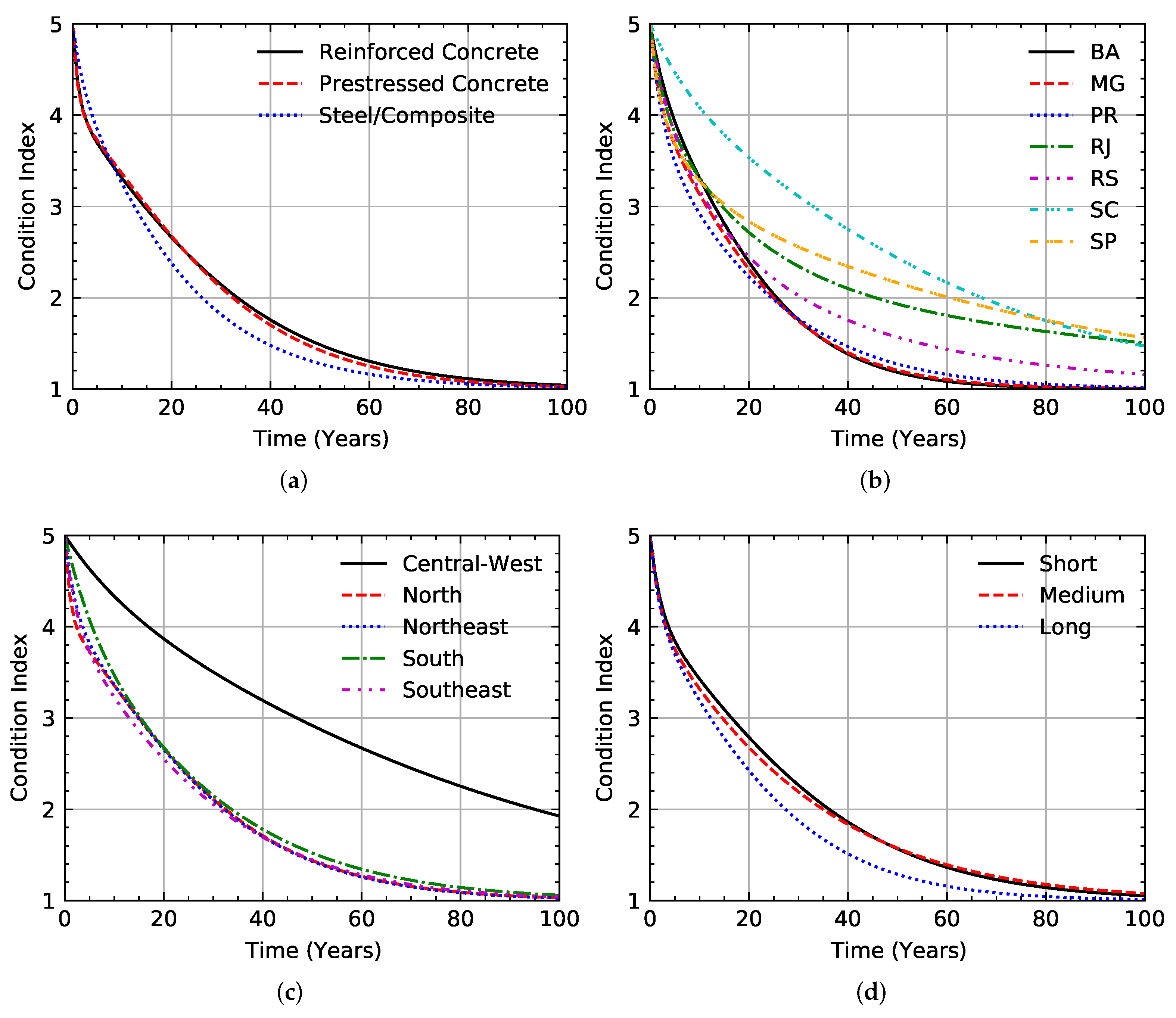
Figure 12a presents the deterioration of bridges with different materials. As observed, reinforced and prestressed concrete bridges have similar deterioration rates, whereas steel and composite bridges have a higher deterioration.
Concerning geographic location, the bridges were categorized by states and regions (
Figure 4) to demonstrate their different performance and lifespan.
Figure 12b shows the deterioration curves for each state, showing no significant difference between states from condition 5 to condition 3. If condition 2 (poor condition in
Table 1) is adopted as the minimum acceptable condition, the predicted average service life of a bridge in BA, RJ, and SP is 25, 45, and 60 years, respectively, with SP presenting the best performance. The anomalous behavior of the SC curve is justified by a high density of inspections with CI equal to 5 in 2015 and 2016, having no further inspections after it. The significant variation of the bridge service life illustrates the considerable impact of the state management policies on the performance of a bridge.
Figure 12c presents the results obtained regarding the regions, where it is possible to observe no significant difference between them, except the central–west region. The only remark, in this case, is the small amount of data that might hinder the actual behavior of this region compared to the others.
Additionally, the bridges were grouped into three categories according to their length. As discussed in
Section 4, the bridges were rated as short (for bridges shorter or equal 30 m), medium (for bridges longer than 30 m and shorter than 60 m), and long (for bridges longer than 60 m). As illustrated in
Figure 12d, longer bridges show a higher deterioration compared to medium and short bridges. This observation is reasonable as it is expected that there is a higher probability of having deterioration in a long bridge than in a short one.
The clustered Markov models reached higher accuracy during testing than the not clustered one, as summarized in
Table 4. It can be observed that the most remarkable improvement was achieved when splitting the data by material type. These results show that adding new features to the model help to improve its performance.
This section has evidenced the influence of selecting a suitable cluster to predict a typical bridge performance. As these predictions are the basis for BMS, inaccuracies might have significant impacts, especially in budget plans. Additionally, carrying out analysis with a fragmented database, as in the case of the Markov model, does not seem to be a good alternative as it can lead to unsafe predictions.
5.2. Artificial Neural Network
Similar to the Markov model analysis, the first assumption was to consider similar deterioration processes for all bridges. For the first ANN model, two input nodes were considered in the input layer, one for the initial CI and the other for the time between inspections (
Figure 9). The optimal configuration for the ANN classifier was determined by trial and error. The inverse of the perplexity (
) was used as an entropy indicator, where a higher rate indicates a lower entropy between the labels and predictions. Accordingly, the final configuration of the ANN is a one-layer network with five hidden neurons in the layer.
Comparing the ANN model against the Markov model, it is possible to observe, in
Table 5, that the ANN model achieved higher accuracy during training, validation, and testing. Even though the test accuracy in the ANN model is slightly lower than the training and validation, the results show that the model could generalize.
With the model calibrated, the performance of the bridge can be evaluated over the years. Three approaches were considered to predict the model throughout the years. For the first approach (
Figure 13a), it is reasonable to assume the extrapolation of up to 100 years. As can be seen, the model could not extrapolate or make predictions outside the training data range. Once it leaves the range for which the model has data, it simply keeps predicting the last known point until it reaches a specific one (40 years), where it drops abruptly. The model cannot generate “new” responses outside of what was seen in the training data.
Another approach to predicting performance over the years is to obtain the transition probability matrix for one year and evaluate the performance over the years, similar to the Markov model.
Figure 13b presents the results for this approach. It is possible to observe that the ANN model yields higher deterioration results. However, it is tricky to consider only one year between inspections when working with the ANN model as it was trained with a time distribution of up to 10 years (
Figure 9).
The final approach considered to obtain the CI through the years was a Monte Carlo (MC) simulation based on the inspection periodicity distribution in
Figure 9. During the simulation, one million artificial bridges were generated with an initial CI equal to 5. For each bridge, a random inspection periodicity was picked from the distribution (
Figure 9) and a new CI was calculated based on the probability from the calibrated model. After all the bridges achieved 100 years, the mean and standard deviation were calculated by year, generating the expected values and confidence interval presented in
Figure 13c. As can be seen, the results from the ANN are now very similar to the Markov results.
5.2.1. Filling the Database by ANN
As it was pointed out, the inspection periodicity as an input parameter can increase the complexity of the ANN model. Therefore, a reasonable strategy is to eliminate it as input by filling the empty inspections in the dataset and making the interval between inspections constant (1 year). Different approaches could be used to reach such desired results. One could assume the bridge maintains the same CI until the next inspection. For example, if a bridge has a CI equal to 4 in 2008 and in the next inspection, in 2011, its CI is equal to 2, the CI assumed for 2009 and 2010 would be 4 for both years. Another approach would be to use a linear interpolation between the inspection records to fill the gap. In this case, the CI for 2009 and 2010 would be 3 and 3.
Even though these approaches could solve the problem, they do not consider the stochastic behavior of the deterioration process. Thus, predictive models such as Markov and ANN would be a better option to fill in the gaps reliably. For the context of this work, and considering the results obtained in
Table 5, the approach selected is the one proposed by [
32], where the authors used an ANN model to generate artificial historical bridge condition indexes. The example already discussed was used to exemplify the application of the selected methodology, as illustrated in
Figure 14.
The final dataset was filled by artificial historical bridge condition indexes generated from a MC simulation using the proposed methodology [
32] and the inspection periodicity distribution in
Figure 9. A total of 4720 data points were generated, inducing the database to go from 12,681 to 17,401 inspections.
5.2.2. Additional Features
Considering the deterioration processes should differ in bridges subjected to different conditions, the model was updated by adding new features one at a time, attempting to improve the results. The new parameters found to be significant to bridge deterioration were the Gross domestic product (GDP), ADTT, total length, and geographic location. For the case of categorical data, one-hot encoding [
21,
23] was used to feed the model.
Figure 15 presents the results for some of the new parameters.
Previously, in the Markov model, the total length was modeled as a categorical parameter. Now, for the case of the ANN model, it has been modeled as a continuum parameter. The results presented in
Figure 15a confirm the same outcome presented in
Figure 12d, where longer bridges show a higher deterioration than shorter bridges. It is important to point out here the advantage of the ANN model, over Markov models, in being able to use continuum inputs instead of only categorical ones.
The results presented earlier in
Figure 12b clarify and help to understand how each state manages its bridges. However, the state is a categorical feature with no natural meaning built into it. In order to view the situation from another perspective, the categorical parameter (states) was converted into an economic continuum parameter (GDP).
Figure 15b illustrates the influence of the GDP. It is possible to observe that states with a higher GDP have a better performance. The significant variation of the bridge service life demonstrates the considerable impact of the GDP on the performance of the bridge. To have an idea of the impact, let us adopt condition 2 (poor condition in
Table 1) as the minimum acceptable condition. By observing
Figure 15b, it is possible to notice that it could vary from 30 years up to 100 years. Additionally, no significant difference from condition 5 to condition 3 was observed.
Some studies [
33,
34] have observed a significant influence of ADTT on bridge performance, by an negative correlation. Thus, it was expected to observe the same results in the analysis carried out. However, as demonstrated in
Figure 15c, the results show a low, or almost zero, influence of ADTT on bridge performance. A possible explanation of why the ADTT did not present the expected results is the fact that the ADTT and the GDP have a positive correlation. In other words, the influence of the GDP might be hiding the influence of ADTT. Another possible reason is that bridges with a high ADTT usually receive more attention from the managers. Further analysis considering the weight and traffic distribution [
35] could help to enhance the results.
The knowledge of the degree of atmospheric aggressiveness is vital in building maintenance management to ensure the project’s useful life [
36]. Humidity and high temperatures notably favor the degradation processes of materials exposed to the atmosphere. Wetting time, type and concentration of gaseous pollutants and particulate matter in the atmosphere determine the magnitude of the attack. The availability of values for these variables greatly assists in assessing the potential risk of corrosion.
Figure 16 illustrates a modified Brooks atmospheric corrosivity index for the Brazilian region.
Although the theoretical conceptualisation in the Brooks index is straightforward, as it only considers humidity and temperature as intervening factors, it can be of value in qualifying the aggressiveness of large rural areas in Brazil, where the data are scarce or nonexistent. On the other hand, when evaluating large cities, industrial areas, and coastal regions, it is essential to be aware that the polluting agents (not considered in the Brooks index [
36]) cause a substantial increase in the corrosion rate.
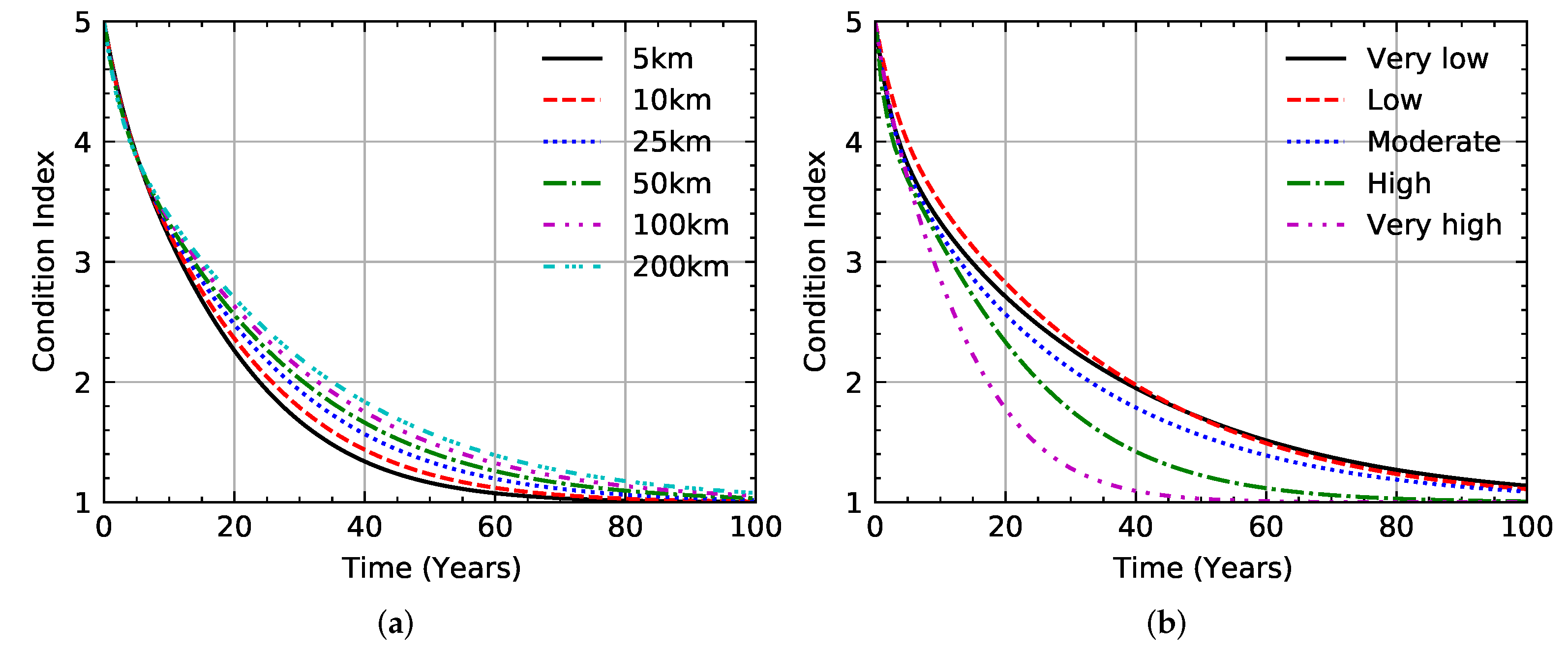
Considering that the location of bridges influences the speed of bridge degradation, particularly for bridges located on the coastal strip, different distances from the coastline were analyzed.
Figure 17a presents the results for coastline distance. As can be observed, the coastline distance significantly influences the deterioration process.
Figure 17b illustrates the influence of each aggressive zone, identifying an additional band (very high) into the map proposed by Brooks (
Figure 16), defined by a distance of less than 5 km from the coast. From
Figure 16, it is possible to conclude that bridges located on the coastline and in the north of Brazil have an unquestionably high deterioration process.
As we are now using a new database, a new analysis not considering any cluster was performed to be used as a reference value. A summary of the results is presented in
Table 6. These results show that adding new features to the model help to improve its performance.
5.2.3. Proof of Concept
A good-quality control plan specifies the extent and the interval of inspections and the data necessary to estimate performance indicators and forecast future development [
4]. In this context, planning is essential to establish a schedule, scope, and optimal times between inspections. As discussed in
Section 2, visual inspection assessment practice differs from standard to standard [
12,
13,
14] when defining the frequency of inspections (periodicity).
The uniform interval approach has resulted in a very costly and inefficient process [
37]. Provisions for adjusting the frequency of routine inspection for certain types or groups of bridges to better conform with their inspection needs have been defined by [
38], taking into account the actual condition index, length, load redundancy, susceptibility to damage, structure type, maintenance history, structure age, ADT, and ADTT. Ref. [
1] developed a framework for risk-based bridge inspection that identifies bridges for which inspection intervals shorter or longer than the one defined by the standards are more appropriate.
According to [
4], the frequency of bridge inspections should depend on bridge condition and bridge importance to the network. Therefore, bridges with poor condition and the most critical bridges should be inspected more frequently than most bridges in the network. On the other hand, new(er) bridges with little or no damage could be inspected less frequently. Additionally, bridges with different material characteristics and locations may require different attention. In order to answer this, bridges with different material characteristics and locations are studied, and their performance is compared.
Six representative groups were selected to represent the case studies, with one bridge representing each corresponding group. Three corrosivity zones (
Figure 16) and the two main materials (
Figure 5) were selected, as shown in
Table 7.
The predicted performance and service life of bridges for each representative group (
Table 7) are presented in
Figure 18. As it can be seen, the bridges have a significant distinction in performance. RC bridges located in a very high corrosive zone have an elevated deterioration process. By adopting condition 2 (poor condition in
Table 1) as the minimum acceptable condition, the predicted average service life for bridges located in the very high corrosive zone is around 20 years, whereas it is 40 years for a very low corrosive zone. The significant variation of the bridge service life illustrates the considerable impact of the corrosive zone on the performance of the bridge, making it almost mandatory to consider the aggressiveness of the region where the bridge is located when defining the periodicity of inspections.
6. Conclusions
The primary contribution of this study to BMS is the application of stochastic models to probabilistically forecast bridge deterioration and the execution of a systematic method to show new features importance in the degradation process, resulting in exciting insights into the definition of inspection periodicity.
The Brazilian standards have different values related to the interval between inspections, but they all consider the periodicity constant, not giving consideration to the bridges’ singularities. As discussed throughout this article, bridges in a network are likely to share similar environmental conditions but, depending on their age, location, structural typology, and other aspects, they may be exposed to different structural deterioration process over time. Hence, forecasting simulations were carried out to identify the bridge behavior for different scenarios.
Two predictive models (Markov and ANN) were created to predict future bridge conditions based on historical data. The most representative up-to-date database of the construction site was served as input for the models, containing information about 10,331 bridges in Brazil from 2008 to 2021.
Considering the deterioration curve obtained for the whole dataset in
Figure 11b and
Figure 13c, the bridges will have, at the end of their 30 years, a condition rating of around 2, if only routine maintenance is performed. Additionally, the forecasting results of two predictive models (Markov and ANN) indicate that the ANN model can predict future conditions more accurately than the Markov one.
In this work, some clusters were identified to improve existing BMS, especially atmospheric corrosivity, which has a significant influence on the deterioration process. The results obtained indicate the proposition of a variation in the periodicity of inspections as a function of the bridges’ degradation curves. While this investigation addressed limited features, other continuous and categorical variables can be added to the methodology (such as the wearing surface and skew angle), which could improve the prediction accuracy of the methodology.
It is essential to emphasize that, regardless of the outstanding potential of Markov and ANN models, the bridge engineer’s opinion must not be ignored. On the contrary, when an expert validates the obtained results, they gain plausibility and can be used confidently.
There is a need to expand and strengthen the works’ inventory to calibrate the results obtained. To achieve this goal, it is necessary to implement joint efforts from all managers, industry professionals, and researchers linked to bridge engineering to promote sharing information, enabling this work to be expanded nationally and internationally.
One limitation of the work is that the results obtained to improve the frequency of inspections are limited to internal factors (deterioration) and do not consider extreme events, such as floods, earthquakes, or any vandalism act.


 ,
, 


