A Multiscale Approach to the Numerical Simulation of the Solid Oxide Fuel Cell

Abstract

The models of solid oxide fuel cells (SOFCs), which are available in the open literature, may be categorized into two non-overlapping groups: microscale or macroscale. Recent progress in computational power makes it possible to formulate a model which combines both approaches, the so-called multiscale model. The novelty of this modeling approach lies in the combination of the microscale description of the transport phenomena and electrochemical reactions’ with the computational fluid dynamics model of the heat and mass transfer in an SOFC. In this work, the mathematical model of a solid oxide fuel cell which takes into account the averaged microstructure parameters of electrodes is developed and tested. To gain experimental data, which are used to confirm the proposed model, the electrochemical tests and the direct observation of the microstructure with the use of the focused ion beam combined with the scanning electron microscope technique (FIB-SEM) were conducted. The numerical results are compared with the experimental data from the short stack examination and a fair agreement is found, which shows that the proposed model can predict the cell behavior accurately. The mechanism of the power generation inside the SOFC is discussed and it is found that the current is produced primarily near the electrolyte–electrode interface. Simulations with an artificially changed microstructure does not lead to the correct prediction of the cell characteristics, which indicates that the microstructure is a crucial factor in the solid oxide fuel cell modeling.

1. Introduction

Fuel cells are electrochemical devices used to convert the chemical energy of a fuel, usually hydrogen, to the electricity directly. Among the fuel cells, the solid oxide fuel cells (SOFCs) are an attractive solution for the future of electric power generation systems in almost all system scales, from small domestic to large industrial generators. Therefore, SOFCs gain more and more attraction in the scientific community. Solid oxide fuel cells utilize good oxygen anions mobility in the elevated temperature (up to 1000 ${}^{\circ }\mathrm{C}$) [1]. The high temperature enables fast electrochemical kinetics without a need to use expensive precious metal catalysts, which is the case of low-temperature fuel cells [2,3]. The high quality of the waste heat makes it possible to install SOFCs in combined heat and power systems. The high operating temperature also allows for converting electrochemically the carbon monoxide or even to conduct the in-stack internal reforming process, which leads to wide fuel flexibility—the variety of reformed hydrocarbons may be used as a fuel for the SOFC [4,5,6]. Among other advantages there are: low emissions of the greenhouse gases (for the hydrogen-fueled fuel cells virtually there is no emissions) and no emissions of the toxic compounds, relatively high tolerance to fuel impurities [7] and outstanding energy conversion efficiency [2]. However, the high operating temperature creates also several problems, especially with the degradation of the materials, corrosion and sealing [1]. This leads to the concept of intermediate temperature solid oxide fuel cells (IT-SOFCs), which work in the temperature range 550 ${}^{\circ }\mathrm{C}$–800 ${}^{\circ }\mathrm{C}$ [8].

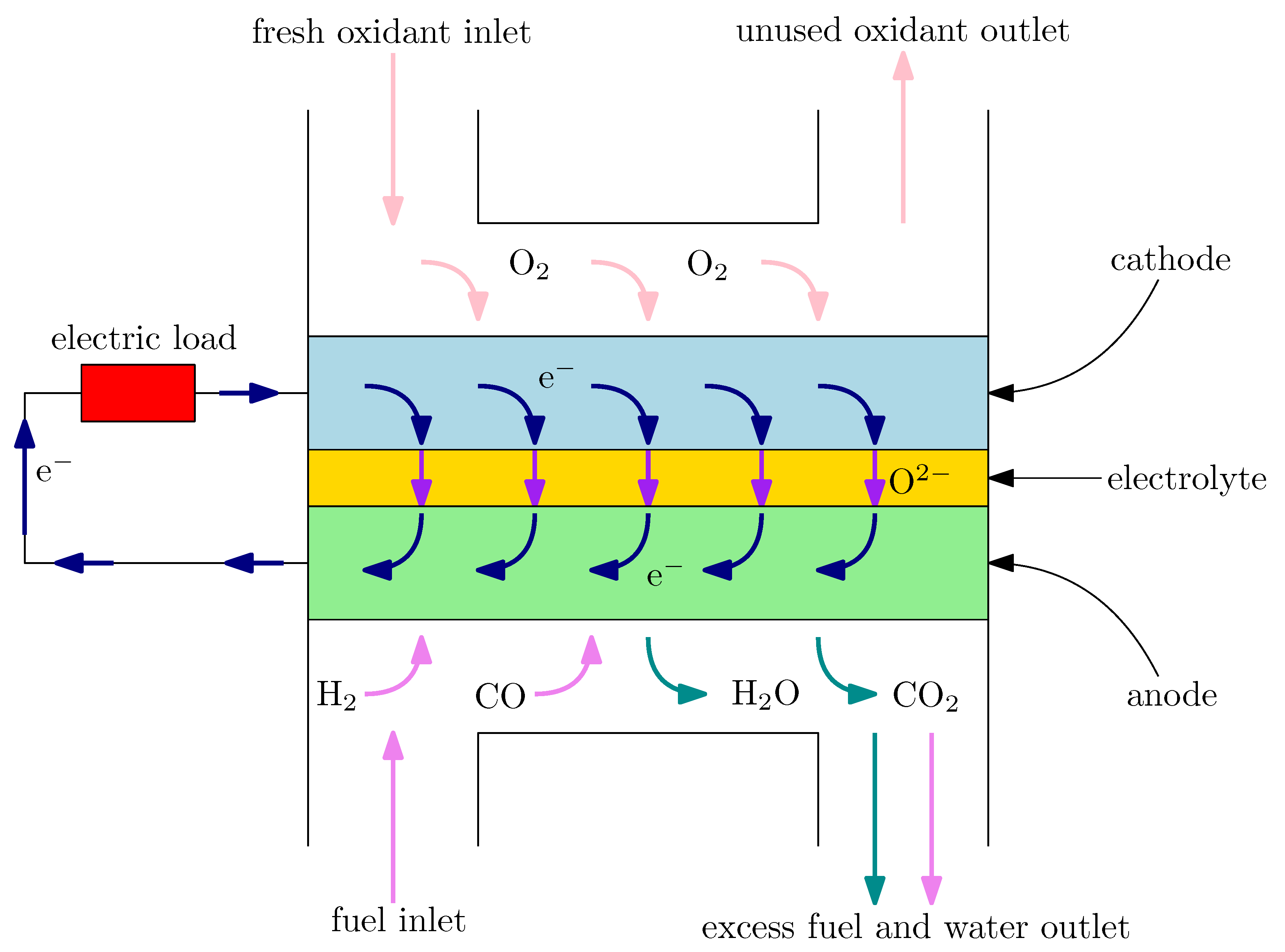
A typical solid oxide fuel cell contains two porous electrodes (an anode and a cathode) and a ceramic solid electrolyte, which separates the electrodes. The schematic diagram of a SOFC is shown in Figure 1. On the anode, the fuel is provided and oxidized according to the following reactions:

• hydrogen oxidation: H₂ + O²⁻ → H₂O + 2 e⁻;
• carbon monoxide oxidation: CO + O²⁻ → CO₂ + 2 e⁻.

The produced electrons are transported through the external circuit to the cathode. On the cathode, the electrons take part in the oxygen reduction reaction: $\frac{1}{2}$ O₂ + 2 e⁻ → O²⁻. The oxygen ions are then conducted to the anode through the electrolyte to oxidize the fuel, which closes the process. The electrodes are characterized by the complex microstructure. For example, the electrochemical reactions can occur only on the sites, where the electron conductor, ion conductor and pore (i.e., “gas conductor”) are in contact. These places are called triple-phase boundaries (TPBs) or—in the case of an electrode material with mixed conductivity (e.g., lanthanum strontium cobalt ferrite (LSCF))—double-phase boundaries (DPBs). The microstructure is a key factor which allows the control of the SOFC performance [9].

Since the construction and testing of novel inventions in the IT-SOFC technology are time-consuming and rather expensive, progress in computational technology and in the methods of mathematical and numerical modeling of solid oxide fuel cells are more and more important. Moreover, the results of numerical models lead to deeper insight into the processes occurring within the SOFC. To analyze the behavior of the SOFCs, usually two classes of the mathematical models are in use. The macroscale models primarily utilize the mass and energy balances or the computational fluid dynamics (CFD) methods to analyze the behavior of the SOFC-based systems [10,11,12], stacks [13,14,15,16] or single cells [17,18,19,20,21]. Moreover, methods such as the finite element (FEM) analysis of thermal stresses [22] or the artificial neural networks [23] are employed. The macroscale models are characterized by the low level of modeling details and usually simplified electrochemistry. This approach allows for representing large-scale systems and to analyze the thermo-fluid behavior of the gases inside the cell. On the other hand, the microscale models focus mainly on the analyses of the mass and charge transport within the single electrode or within the PEN (positive electrode–electrolyte–negative electrode) assembly. The microscale models employ a variety of methods, such as the models based on the finite volume solution of partial differential equations [24,25,26], the models which implement the Lattice–Boltzmann method (LBM) [27,28,29], the sub-grid scale models [30], the random resistor network models [31] or the kinetic Monte Carlo models [32]. A greater amount of modeling details allows for describing the behavior of the electrode very accurately. However, because of the large computational cost, the simulation of the whole cell is a difficult task. Moreover, microscale models usually do not include energy transport.

It is possible to combine the macro- and microscale approach and to form a hybrid multiscale model [33], which focuses on the interaction between unit performance and the microstructure of the electrodes. Multiscale models allow for simulating the cell behavior very accurately and to observe the impact of the microstructure on a cell or even a SOFC stack performance. Because of the large complexity and high computational cost, there have been a few attempts to develop the multiscale model. For example, Ho et al. prepared the multiscale model in STAR-CD software (version 3.24, CD-Adapco Group, Melville, NY, USA) [34]. The authors did not mention, from where they took the microstructural data. Moreover, they state that the amount of experimental data needed to confirm the numerical models of the SOFCs are rare in the literature. Sohn et al. published a two-dimensional multiscale model of an anode-supported SOFC [35]. The synthetic microstructure is constructed using the random binary packing algorithm and only the electrochemical model is verified with the experimental data. Both models are not used to check the impact of the different microstructure. Brus et al. presented a two-dimensional isothermal model of the PEN [36]. The averaged electrodes’ microstructure parameters were taken from thefocused ion beam/scanning electron microscopy (FIB-SEM) measurements, and the set of the experimental results from the short stack is presented. The model does not take into account the flow in the gas channels.

As can be seen from the literature review, complex multiscale models are rare and these models are significantly simplified. According to the knowledge of the authors, there is no experimentally confirmed non-isothermal multiscale model, which use a real microstructure data. In this work, we want to develop and to make an attempt to falsify the non-isothermal multiscale model of a single planar SOFC. A mathematical model cannot be proved to be true; however, if the experimental and numerical data are in agreement, the model may be accepted as a verified, which is a goal of the falsification procedure [37]. To reach this aim, we performed the electrochemical tests of the short stack of solid oxide fuel cells to gain a unique set of data. Next, the samples of the analyzed cells’ electrodes were observed in three dimensions using the FIB-SEM technique. Collected images are used for the quantification of microstructural parameters, which are implemented into the numerical model. The numerical results from the proposed model are compared with the experimental data. On the basis of the numerical results, we discuss the power generation process in order to achieve a better understanding of the SOFC physics. To demonstrate the importance of the microstructure, the simulation with the different microstructure is provided. We also believe that the experimental and microstructural data presented in this work help to form the benchmark for future numerical simulations of the SOFCs.

2. Experimental Examination of the SOFC Stack

To gain the set of experimental data to verify the mathematical model or to make a falsification attempt, electrochemical measurements of the SOFC short stack were performed. The static current–voltage and current–power characteristics are presented. The results show the response of the solid oxide fuel cell to the different operating temperature and the different fuel composition.

2.1. Experimental Set-Up

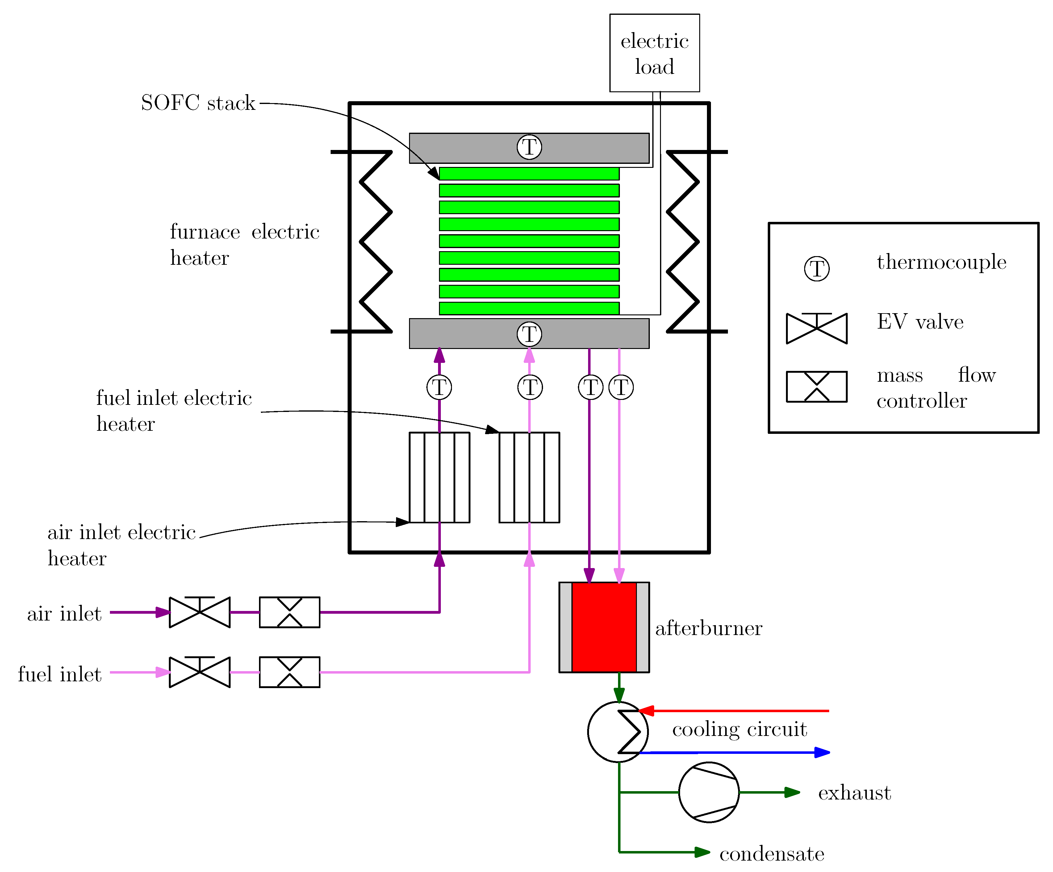
The test module for the SOFC stacks used in this study is the modular stack test bench (MSTB), designed and manufactured by the SOLIDPower S.p.a. The set-up was located in Department of Fundamental Research in Energy Engineering, AGH University of Science and Technology, Krakow, Poland. The scheme of the MSTB is shown on Figure 2. Inside the MSTB furnace, the short stack of the nine solid oxide fuel cells, provided by the SOLIDPower S.p.a., was enclosed. Every one of the cells is a planar SOFC, with the solid electrolyte fabricated from yttria-stabilized zirconia (YSZ), the anode made from Ni/YSZ cermet. The layered cathode is fabricated from the gadolinium-doped ceria (GDC) (buffer layer), the LSCF/GDC composite (functional layer) and the pure LSCF perovskite (current collector layer). The thicknesses of the components of every one of the cells are shown in

Table 1. Thicknesses of the cell components.

Element	Anode	Electrolyte	Cathode	Anode Channel	Cathode Channel
Thickness [$\mathsf{\mu }$m]	240	10	50	700	1400

.

Table 2. Layers of the cathode.

Layer	Buffer Layer	Active Layer	Current Collector Layer	Total
Thickness [$\mathsf{\mu }$m]	0.5	9.5	40	50

presents the layered composition of the cathode. The cells have the active area 6 × 8 ${\mathrm{cm}}^2$. The electric load device allows for controlling the current withdrawn from the stack. The air and fuel are supplied through the electromagnetic valves, the mass flow controllers and the inlet heaters to the stack. The products of the electrochemical reactions, unused fuel and air are mixed together and burned in the afterburner. The leftovers are cooled down and the condensate and exhaust are released. The temperature inside the MSTB is controlled by six thermocouples, marked in Figure 2 with Ⓣ, and the driver software, MSTestBench (version 15, SOLIDPower S.p.a., Mezzolombardo, Italy), is used to operate the testing system. The operating conditions of the MSTB are shown in

Table 3. Modular stack test bench operating conditions.

fuel flow rate	$2.6\mathrm{L}{\min }^{-1}$
fuel pressure	3 $\mathrm{bar}$
fuel inlet heater temperature	350 ${}^{\circ }\mathrm{C}$
air flow rate	$28.8\mathrm{L}{\min }^{-1}$
air pressure	5 $\mathrm{bar}$
air inlet heater temperature	550 ${}^{\circ }\mathrm{C}$
afterburner temperature	400 ${}^{\circ }\mathrm{C}$

. The temperatures of the inlet electric heaters and of the afterburner are constant during the operation. The total flow rate should also be constant, however, the amount of the hydrogen and nitrogen in the fuel mixture may vary. To avoid fuel starvation, the amount of hydrogen in the fuel should always be less than 70%. Due to safety reasons, the potential of the stack should not fall below $5.4$ $\mathrm{V}$, to avoid operation in the concentration overpotential region. Only the total potential or voltage of the stack is measured. The cell power density $p_{\mathrm{out}}$ ($\mathrm{W}\mathrm{c}{\mathrm{m}}^{-2}$) may be calculated using the following formula:

$$p_{\mathrm{out}}={\displaystyle \frac{IE}{A_{\mathrm{cell}}}},$$

(1)

where I ($\mathrm{A}$) is the current withdraw from the cell, E ($\mathrm{V}$) is the average cell potential and $A_{\mathrm{cell}}$ stands for the cell active area ($\mathrm{c}{\mathrm{m}}^2$). If not indicated otherwise, the molar fraction of nitrogen is given as ${\chi }_{{\mathrm{N}}_2}=1.0-{\chi }_{{\mathrm{H}}_2}$.

2.2. Experimental Results

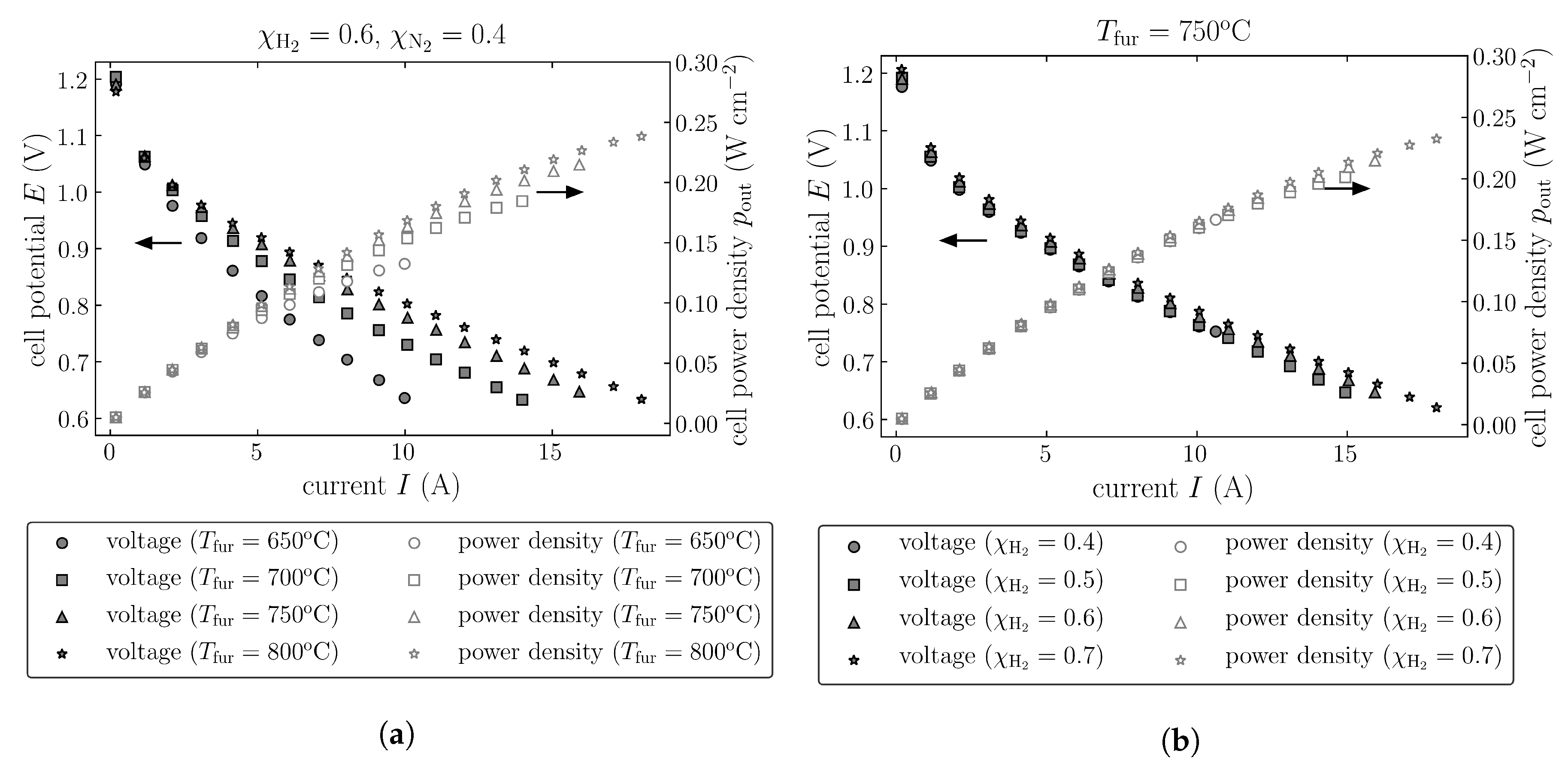
The relations between the current, voltage and power for the stack, which works under the different furnace temperature—which determines the stack operating temperature—and under the different fuel composition (i.e., concentration of the hydrogen and nitrogen at the stack inlet) have been examined. The experimental results are presented as the current–voltage and current–power characteristics, since many parametric studies on the SOFCs focus on these relations. The results are shown in Figure 3.

As shown in Figure 3a, increasing furnace temperature leads to the higher voltage at the same load. The difference between the cell potential at the temperature 650 ${}^{\circ }\mathrm{C}$ and 800 ${}^{\circ }\mathrm{C}$ and at the load 10 $\mathrm{A}$ is almost $0.2$ $\mathrm{V}$. The power in the further case is around $0.05$ $\mathrm{W}$ ${\mathrm{cm}}^{-2}$ higher. This effect is caused by the faster electrochemical kinetics and increased ionic conductivity of the YSZ in the higher temperature. The performance of the stack experiences a relatively large increase between 650 ${}^{\circ }\mathrm{C}$ and 700 ${}^{\circ }\mathrm{C}$, whereas the performance is only slightly higher between 700 ${}^{\circ }\mathrm{C}$ and 800 ${}^{\circ }\mathrm{C}$ (see Figure 3a).

Figure 3b presents the results for the different inlet fuel composition. As can be observed, the higher fraction of hydrogen in the fuel leads to slightly better performance and higher power. Nevertheless, the effect of the hydrogen concentration in the fuel is not as significant as the effect of temperature. Please note that the lower the molar fraction of hydrogen is in the fuel mixture, the higher is the utilization factor; therefore, for the fuel with ${\chi }_{{\mathrm{H}}_2}=0.4$, the maximum achieved power density is lower than for the case with the fuel containing ${\chi }_{{\mathrm{H}}_2}=0.7$.

3. Microstructure Analysis and Quantification

The dual beam microtomography based on the focused ion beam and scanning electron microscopy (FIB-SEM) is a technique, which can be used to examine the complex microstructure of the porous materials, for example electrodes of a solid oxide fuel cell. The first FIB-SEM three-dimensional reconstruction of the SOFC anode was reported by Wilson et al. in 2006 [38], since this year the number of scientific papers which focus on the FIB-SEM observation of the SOFC’s electrodes increase [28,36,39,40,41]. To gain unique data about the microstructure of the cells investigated empirically (see Section 2.2), the FIB-SEM method is used here.

3.1. Sample Preparation and FIB-SEM Observation

The representative samples of the anode and the cathode functional layer were taken from the investigated short stack (see Section 2). Since the structure of the electrodes is porous, the pores were impregnated with EpoFix resin (Struers) under vacuum conditions, in order to achieve the recognition of the pores on the SEM images. Next, the samples were cut and polished with sand paper and diamond paste.

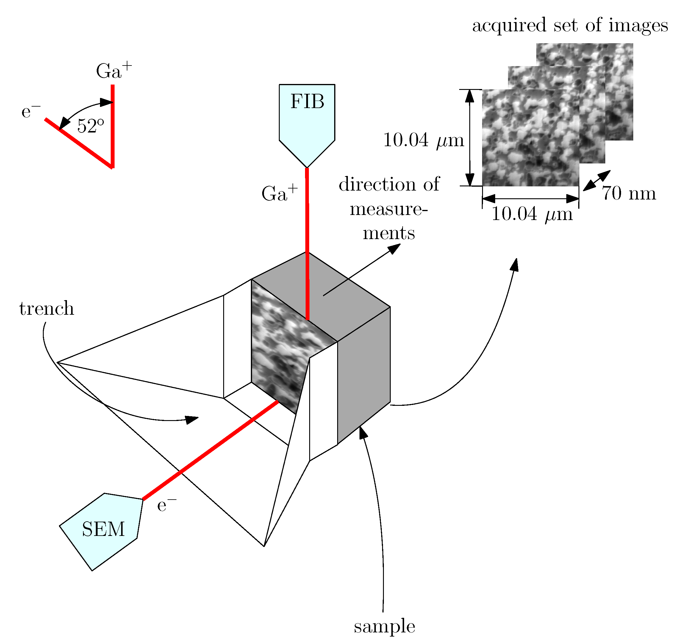
The observation of the electrodes’ microstructure was conducted on the FEI Versa 3D Dual Beam FIB-SEM apparatus, located in Academic Centre for Materials and Nanotechnology, AGH University of Science and Technology, Krakow, Poland. Figure 4 shows the scheme of the FIB-SEM setup. The “cut-and-see” observation procedure is as follows:

• A trench is prepared by the focused beam of Ga⁺ ions (FIB).
• The intersection of an electrode is photographed with the SEM.
• The FIB mills the thin layer of the electrode and exposes the next intersection.
• The procedure is continued until the whole volume of interest is imaged.

As a result, the set of 2D SEM images is acquired. The 3D reconstruction of the electrodes is obtained by the resampling, cropping, aligning and stacking of the images in the 3D space.

3.2. Segmentation of the Microstructure

The SEM images were resampled, cropped, stacked and aligned in the Avizo 3D analysis software (version 9.2.0, FEI, Hillsboro, OR, USA). However, the result is a set of raw images, with no information about the phases. Therefore, the segmentation procedure is required. The segmentation is a process of assigning every one of the voxels from the images stack to one of the electrodes’ structural phases.

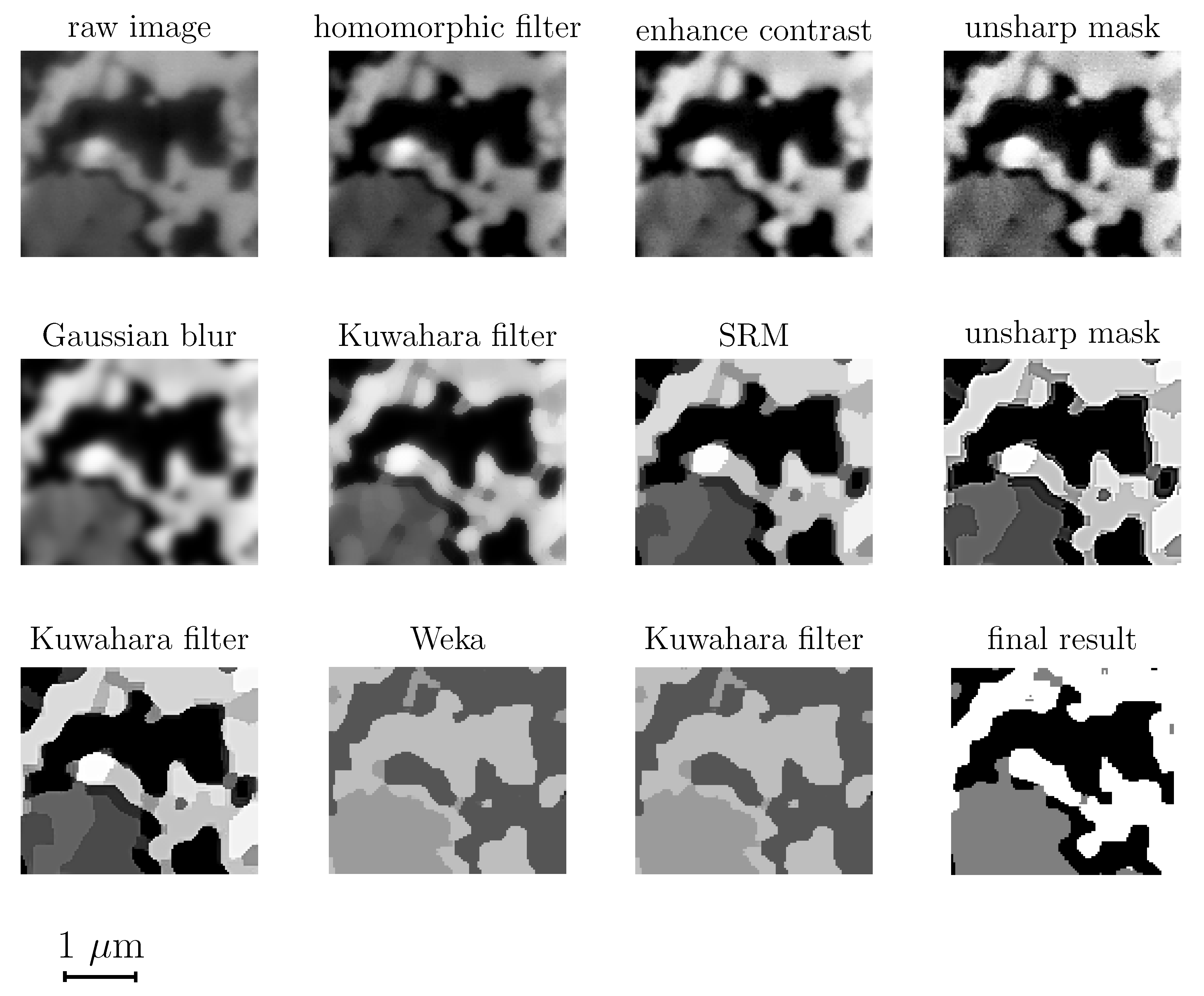
The segmentation is often done manually. This is a difficult and time-consuming task. Therefore, we want to propose a simple framework for the semi-automatic segmentation procedure. The Fiji distribution of the open source image analysis software ImageJ (version 1.52i, National Institutes of Health, Bethesda, MD, USA) [42,43] is primarily used to perform this task, together with the several in-home scripts in the Python programming language, with an extensive use of the scikit-image image processing library [44]. The procedure is illustrated in Figure 5 on an example of the cathode segmentation. The semi-automatic segmentation algorithm, shown in Figure 5, may be summarized as follows:

• The homomorphic filter [45] with the high- and low-frequency filters (${\gamma }_1=0.1$, ${\gamma }_2=0.25$) and the Gaussian filter ($\sigma =10$) is applied in order to equalize the brightness of the images (in-house script).
• The enhance contrast tool (with options: normalize, equalize histogram, use stack histogram) is used to underline the differences between the phases (Fiji).
• The unsharp masking ($\sigma =1.0$, mask weight 0.6) is utilized to sharpen the image (Fiji).
• The Gaussian blur ($\sigma =2.0$) is used in order to remove the artifacts, which appear at the phase boundaries (Fiji).
• The Kuwahara filter (sampling window 5) is exploited to smooth the images and to remove further artifacts (Fiji).
• The statistical region merging algorithm ($Q=30$) [46] is used for the initial recognition of the phases (Fiji).
• The unsharp masking and the Kuwahara filter with parameters the same as the above are applied to the images (Fiji).
• The Trainable Weka Segmentation tool (version 3.2.32, see Reference [47] for further details), which utilize the artificial neural networks and machine learning algorithms to automatically segment the images, is used to recognize the phases (Fiji). The following training features were chosen: Gaussian blur (${\sigma }_{\min }=1.0$, ${\sigma }_{\max }=8.0$), Laplacian, Hessian, Structure, and Edges. The fast version of the random forests machine learning algorithm is utilized to recognize the phases. The Weka software requires some training data, therefore a few images were segmented manually.
• The Kuwahara filter is applied again (Fiji).
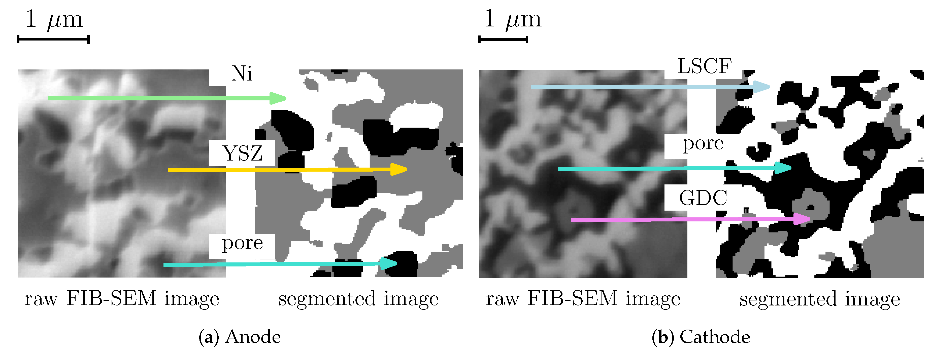
• The image is recolored (the following color levels in the grayscale are required for the quantification algorithms: anode—pore 0, YSZ 127, Ni 256; cathode—pore 0, GDC 127, LSCF 256) and the bad pixels are removed (in-house script).

The samples of the raw FIB-SEM images and the segmented images are presented in Figure 6. The result images were visually compared with the raw SEM photographs and good agreement was found.

3.3. Quantification of the Microstructure

Based on the obtained set of the segmented images, the three-dimensional digital representations of the electrodes’ microstructure were prepared in the Avizo 3D software. Three-dimensional representations of the microstructure of the anode and cathode are presented in Figure 7.

Table 4. Sample sizes and voxel sizes.

Sample	Sample Size [$\mathsf{\mu }$m]			Voxel Size [nm]
	$\mathit{x}$	$\mathit{y}$	$\mathit{z}$	$\mathit{x}$	$\mathit{y}$	$\mathit{z}$
anode	10.04	10.04	10.43	26.98	26.98	70.00
cathode	10.33	10.33	10.92	38.54	38.54	70.00

shows the volume of the reconstructed samples and the voxel sizes. Based on the segmented images, the averaged microstructural parameters are derived.

3.3.1. Volume Fraction and Mean Particle Diameter

The volume fraction $\psi$ was calculated by counting off the voxels which belong to each phase. The percentage of the voxels which belong to the phase of interest to the total number of voxels was computed [36,41]. The mean diameters of the solid particles and pores $\overline{d}$ were evaluated using the three-dimensional version of the line intercept method (see [48] for the details of the procedure). The results are shown in

Table 5. Volume fractions and mean particle diameters of each phase.

Anode
phase	Ni	YSZ	pore
volume fraction$\psi$	0.33	0.41	0.26
mean diameter$\overline{d}$ [$\mathsf{\mu }\mathrm{m}$]	0.77	0.81	0.71
Cathode
phase	LSCF	GDC	pore
volume fraction$\psi$	0.34	0.27	0.39
mean diameter $\overline{d}$ [$\mathsf{\mu }\mathrm{m}$]	1.00	1.30	1.02

.

3.3.2. Tortuosity Factors

The tortuosity factors $\tau$ are calculated using the random walking algorithm. The computations are based on the fact, that the mean square displacements of the random walkers and—what follows—the diffusion coefficients are lower in the porous structure than in the void space. The degree of the reduction of the diffusion coefficients is interpreted as the tortuosity factors. The details of the algorithm can be found in [41,49]. The calculated tortuosity factors are shown in

Table 6. Tortuosity factors of each phase.

Phase	Tortuosity Factor $\mathit{\tau }$
anode
Ni	3.647
YSZ	2.240
pore	24.534
cathode
LSCF	3.953
GDC	10.324
pore	2.419

.

3.3.3. Phase Boundaries’ Densities

The computation of the phase boundaries’ densities was performed in the Avizo software. The results are shown in

Table 7. Effective phase boundaries’ densities.

anodic TPB length density${\rho }_{\mathrm{TPB},\mathrm{ano}}^L$ [$\mathsf{\mu }\mathrm{m}\mathsf{\mu }{\mathrm{m}}^{-3}$]	4.44
cathodic TPB length density${\rho }_{\mathrm{TPB},\mathrm{cath}}^L$ [$\mathsf{\mu }\mathrm{m}\mathsf{\mu }{\mathrm{m}}^{-3}$]	2.11
cathodic DPB area density${\rho }_{\mathrm{DPB},\mathrm{cath}}^A$ [$\mathsf{\mu }{\mathrm{m}}^2\mathsf{\mu }{\mathrm{m}}^{-3}$]	1.63

.

4. Mathematical Model

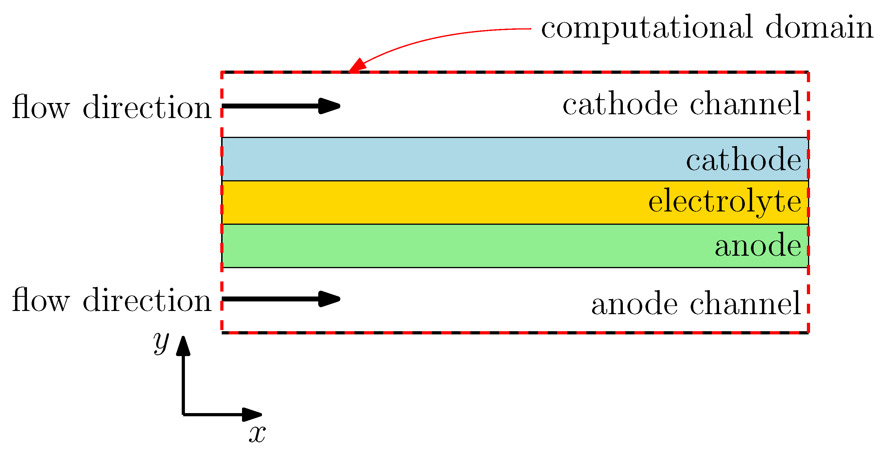
The steady mathematical model is based on the set of partial differential equations and the Butler–Volmer electrochemical model, with the inclusion of the averaged microstructure parameters (see Section 3). The computational domain is shown on Figure 8. In this model, it is assumed that the computational domain is divided into five subdomains: the cathode and anode channels, the cathode, the electrolyte and the anode. The dimensions of the subdomains are the same as for the cells investigated experimentally (see Table 1). The porous anode is fabricated from the Ni/YSZ and the solid electrolyte is made from the YSZ. The layered structure of the cathode is neglected and it is assumed that the cathode is made from the pure LSCF. Because the GDC is not introduced in the model, the microstructure was recalculated for the pure LSCF cathode (for the recalculation, it was assumed that the analyzed cathode, shown in Figure 7b, is composed of the single LSCF phase). Such an assumption leads to an unavoidable error in the numerical results. Having said that, the cathodic voltage losses are usually lower than the anodic polarization losses [36]. Moreover, at the elevated temperature (>$650{}^{\circ }\mathrm{C}$), the LSCF/GDC behavior is similar to the pure LSCF performance [50]. The results are presented in

Table 8. Reference microstructure for the numerical calculations.

Parameter	Reference Microstructure
${\psi }_{\mathrm{pore},\mathrm{ano}}$	0.26
${\psi }_{\mathrm{Ni}}$	0.33
${\psi }_{\mathrm{YSZ}}$	0.41
${\psi }_{\mathrm{pore},\mathrm{cath}}$	0.39
${\psi }_{\mathrm{LSCF}}$	0.61
${\tau }_{\mathrm{pore},\mathrm{ano}}$	24.534
${\tau }_{\mathrm{Ni}}$	3.647
${\tau }_{\mathrm{YSZ}}$	2.240
${\tau }_{\mathrm{pore},\mathrm{cath}}$	2.419
${\tau }_{\mathrm{LSCF}}$	1.850
$d_{\mathrm{pore},\mathrm{ano}}$ ($\mathsf{\mu }\mathrm{m}$)	0.71
$d_{\mathrm{pore},\mathrm{cath}}$ ($\mathsf{\mu }\mathrm{m}$)	1.02
${\rho }_{\mathrm{TPB},\mathrm{ano}}^L$ ($\mathsf{\mu }\mathrm{m}\mathsf{\mu }{\mathrm{m}}^{-3}$)	4.44
${\rho }_{\mathrm{DPB},\mathrm{cath}}^A$ ($\mathsf{\mu }{\mathrm{m}}^2\mathsf{\mu }{\mathrm{m}}^{-3}$)	2.59

.

The gases in the system are treated as the Newtonian ideal gases, and the radiation heat transfer, viscous dissipation, gravity and other body forces are neglected. It is also assumed that, at the anode inlet, only hydrogen, water vapor and nitrogen are present, whereas, in the cathode inlet, air containing 21% of the oxygen and 79% of the nitrogen is provided. Please note that the model presented here is based on our previous isothermal model of the PEN [36].

4.1. Thermo-Electric Model

The thermo-electric model describes the thermodynamics and the electrochemistry of the SOFC. The hydrogen-fueled SOFC realizes the following reactions:

• the anodic reaction—hydrogen oxidation: H₂ + O²⁻ → H₂O + 2 e⁻;
• the cathodic reaction—oxygen reduction: $\frac{1}{2}$ O₂ + 2 e⁻ → O²⁻;
• the overall cell reaction: H₂ + $\frac{1}{2}$ O₂ → H₂O.

These reactions may occur only at the sites, where the constant supply and drain of the reactants and products are possible. These reaction sites are called the triple phase boundaries (TPBs) on the anode and the double phase boundaries (DPBs) on the cathode. Please mind that the cathodic TPB is neglected in this model.

The open circuit voltage of such a cell may be described by the Nernst equation. For the cell working in any temperature and pressure, the Nernst equation may be written as [3]:

$$E_{\mathrm{OC}}=-{\displaystyle \frac{{\Delta }_{{\mathrm{H}}_{2}x{\mathrm{O}}_2}{g}^{⦵}}{2F}}+{\displaystyle \frac{{\Delta }_{{\mathrm{H}}_{2}x{\mathrm{O}}_2}s}{2F}}\left(T-T^{⦵}\right)-{\displaystyle \frac{RT}{2F}}ln\left({\displaystyle \frac{p_{{\mathrm{H}}_2\mathrm{O}}}{p_{{\mathrm{H}}_2}{p}_{{\mathrm{O}}_2}^{\raisebox{1ex}{$1$}\!\left/ \!\raisebox{-1ex}{$2$}\right.}}}\right),$$

(2)

where $E_{\mathrm{OC}}$ ($\mathrm{V}$) is the open circuit voltage of the SOFC, ${\Delta }_{{\mathrm{H}}_{2}x{\mathrm{O}}_2}{g}^{⦵}$ ($\mathrm{J}{\mathrm{mol}}^{-1}$) is the specific molar Gibbs free energy of the water formation in the standard state (here, the standard state temperature is $T^{⦵}=298\mathrm{K}$ and the standard state pressure is $P^{⦵}$ = 101,325 Pa = 1 atm), ${\Delta }_{{\mathrm{H}}_{2}x{\mathrm{O}}_2}s$ ($\mathrm{J}{\mathrm{mol}}^{-1}{\mathrm{K}}^{-1}$) is the change of the specific molar entropy associated with the water formation reaction, T ($\mathrm{K}$) is the temperature and $p_i$ ($\mathrm{atm}$) stands for the partial pressure of species i. F is the Faraday constant (F = 96,485.32289 C mol${}^{-1}$) and R is the universal gas constant ($R=8.3144598\mathrm{J}{\mathrm{mol}}^{-1}{\mathrm{K}}^{-1}$).

To calculate the volumic current density, generated at the triple phase boundaries (on the anode) $j_{\mathrm{TPB}}^{\mathrm{ano}}$ ($\mathrm{A}{\mathrm{m}}^{-3}$) and the double phase boundaries (on the cathode) $j_{\mathrm{DPB}}^{\mathrm{cath}}$ ($\mathrm{A}{\mathrm{m}}^{-3}$), the Butler–Volmer equations are utilized:

anode:

$$\begin{array}{cc}\hfill j_{\mathrm{TPB}}^{\mathrm{ano}}& =j_0^{\mathrm{ano},\mathrm{TPB}}{\rho }_{\mathrm{TPB}}^L\left[exp\left({\displaystyle \frac{1.4F}{RT}}{\eta }_{\mathrm{act}}\right)-exp\left(-{\displaystyle \frac{0.8F}{RT}}{\eta }_{\mathrm{act}}\right)\right],\hfill \end{array}$$

(3a)

cathode:

$$\begin{array}{cc}\hfill j_{\mathrm{DPB}}^{\mathrm{cath}}& =j_0^{\mathrm{cath},\mathrm{DPB}}{\rho }_{\mathrm{DPB}}^A\left[exp\left({\displaystyle \frac{1.2F}{RT}}{\eta }_{\mathrm{act}}\right)-exp\left(-{\displaystyle \frac{F}{RT}}{\eta }_{\mathrm{act}}\right)\right].\hfill \end{array}$$

(3b)

Here, $j_0^{ano,TPB}$ ($\mathrm{A}{\mathrm{m}}^{-1}$) is the exchange current density per unit length of the TPB and $j_0^{cath,DPB}$ ($\mathrm{A}{\mathrm{m}}^{-2}$) is the exchange current density per unit area of the DPB; ${\rho }_{\mathrm{TPB}}^L$ (${\mathrm{m}}^3{\mathrm{m}}^{-1}$) is the TPB length density and ${\rho }_{\mathrm{DPB}}^L$ (${\mathrm{m}}^3{\mathrm{m}}^{-2}$) is the DPB area density. The anodic and cathodic charge-transfer coefficients are taken from the porous Ni/YSZ anode measurements of de Boer [51] and from the LSCF cathode investigation of Fleig et al. [52]. The activation overpotentials ${\eta }_{\mathrm{act}}$ ($\mathrm{V}$) are calculated as follows:

anode:

$$\begin{array}{cc}\hfill {\eta }_{\mathrm{act}}^{\mathrm{ano}}& ={\varphi }_{\mathrm{el}}^{\mathrm{ano}}-{\varphi }_{\mathrm{ion}}^{\mathrm{ano}}-{\displaystyle \frac{RT}{2F}}ln\left({\displaystyle \frac{p_{{\mathrm{H}}_2}^{\mathrm{bulk}}}{p_{{\mathrm{H}}_2}}}{\displaystyle \frac{p_{{\mathrm{H}}_2\mathrm{O}}}{p_{{\mathrm{H}}_2\mathrm{O}}^{\mathrm{bulk}}}}\right),\hfill \end{array}$$

(4a)

cathode:

$$\begin{array}{cc}\hfill {\eta }_{\mathrm{act}}^{\mathrm{cath}}& ={\varphi }_{\mathrm{ion}}^{\mathrm{cath}}-{\varphi }_{\mathrm{el}}^{\mathrm{cath}}-{\displaystyle \frac{RT}{4F}}ln\left({\displaystyle \frac{p_{{\mathrm{O}}_2}^{\mathrm{bulk}}}{p_{{\mathrm{O}}_2}}}\right).\hfill \end{array}$$

(4b)

In Equations (4a) and (4b), the symbols ${\varphi }_{\mathrm{el}/\mathrm{ion}}$ ($\mathrm{V}$) are the electric potentials of the electronic and ionic conducting phases, $p_i$ ($\mathrm{Pa}$) means the partial pressure of species i, and the superscript $\mathrm{bulk}$ indicates that the partial pressure value is the bulk inlet partial pressure.

The exchange current densities per unit length of the TPB/unit area of the DPB are formulated in accordance with the literature data [51,53]. The pre-exponential factors are the fitting parameters, proposed by Suzue et al. (for the andoe) [27] and Matsuzaki et al. (for the cathode) [28]. The exchange current densities are calculated as:

anode:

$$\begin{array}{cc}\hfill j_0^{\mathrm{ano},\mathrm{TPB}}& =31.4p_{{\mathrm{H}}_2}^{-0.06}{p}_{{\mathrm{H}}_2\mathrm{O}}^{0.43}exp\left(-{\displaystyle \frac{\mathrm{152,000}}{RT}}\right),\hfill \end{array}$$

(5a)

cathode:

$$\begin{array}{cc}\hfill j_0^{\mathrm{cath},\mathrm{DPB}}& =1.47·{10}^6·p_{{\mathrm{O}}_2}^{0.23}exp\left(-{\displaystyle \frac{\mathrm{133,150}}{RT}}\right),\hfill \end{array}$$

(5b)

where the partial pressures $p_i$ are taken in pascals.

4.2. Transport Model

The transport model is based on the set of the partial differential equations, which describe species, energy and charge conservation. In addition, the equation of the state—here the ideal gas law—is used:

$$Pv={\displaystyle \frac{R}{M}}T,$$

(6)

where P ($\mathrm{Pa}$) is the total pressure, v (${\mathrm{m}}^3{\mathrm{k}\mathrm{g}}^{-1}$) is the specific volume, M ($\mathrm{k}\mathrm{g}{\mathrm{mol}}^{-1}$) is the molar mass and T ($\mathrm{K}$) is the temperature.

The velocity $u\left(y\right)$ inside the gas channels is described by the following form of the Darcy–Brinkmann equation [54], obtained for the fully-developed, one-dimensional, axial, incompressible flow:

$${\displaystyle \frac{\mathrm{d}P}{\mathrm{d}x}}=\mu \epsilon {\displaystyle \frac{{\mathrm{d}}^{2}u}{\mathrm{d}{y}^2}}-{\displaystyle \frac{\epsilon \mu }{K}}u.$$

(7)

This partial differential equation is possible to be solved analytically with the no-slip boundary conditions. Moreover, the pressure gradient may be replaced by the mass flow rate, defined as $\dot{m}=\rho W{\int }_0^{H}u\left(y\right)\mathrm{d}y$. The velocity profile is then described by:

$$u\left(y\right)={\displaystyle \frac{\dot{m}}{\rho W}}{\displaystyle \frac{f\left(y\right)}{C}}.$$

(8)

The function $f\left(y\right)$ in Equation (8) is given by:

$$f\left(y\right)={\displaystyle \frac{1-exp\left(-H{K}^{-\raisebox{1ex}{$1$}\!\left/ \!\raisebox{-1ex}{$2$}\right.}\right)}{2sinh\left(H{K}^{-\raisebox{1ex}{$1$}\!\left/ \!\raisebox{-1ex}{$2$}\right.}\right)}}exp\left(y{K}^{\raisebox{1ex}{$1$}\!\left/ \!\raisebox{-1ex}{$2$}\right.}\right)+\left(1-{\displaystyle \frac{1-exp\left(-H{K}^{-\raisebox{1ex}{$1$}\!\left/ \!\raisebox{-1ex}{$2$}\right.}\right)}{2sinh\left(H{K}^{-\raisebox{1ex}{$1$}\!\left/ \!\raisebox{-1ex}{$2$}\right.}\right)}}\right)exp\left(-y{K}^{\raisebox{1ex}{$1$}\!\left/ \!\raisebox{-1ex}{$2$}\right.}\right)-1,$$

(9)

and the constant C, which appears in Equation (8), is evaluated as follows:

$$\begin{array}{c}C={\displaystyle \frac{1-exp\left(-H{K}^{-\raisebox{1ex}{$1$}\!\left/ \!\raisebox{-1ex}{$2$}\right.}\right)}{2sinh\left(H{K}^{-\raisebox{1ex}{$1$}\!\left/ \!\raisebox{-1ex}{$2$}\right.}\right)}}\sqrt{K}\left(exp\left(H{K}^{-\raisebox{1ex}{$1$}\!\left/ \!\raisebox{-1ex}{$2$}\right.}\right)-1\right)\hfill \\ \hfill -\left(1-{\displaystyle \frac{1-exp\left(-H{K}^{-\raisebox{1ex}{$1$}\!\left/ \!\raisebox{-1ex}{$2$}\right.}\right)}{2sinh\left(H{K}^{-\raisebox{1ex}{$1$}\!\left/ \!\raisebox{-1ex}{$2$}\right.}\right)}}\right)\sqrt{K}\left(exp\left(-H{K}^{-\raisebox{1ex}{$1$}\!\left/ \!\raisebox{-1ex}{$2$}\right.}\right)-1\right)-H.\end{array}$$

(10)

In the above equations, $\dot{m}$ ($\mathrm{k}\mathrm{g}{\mathrm{s}}^{-1}$) is the mass flow rate, $\rho$ is the averaged cross-sectional density, calculated with the ideal gas law (Equation (6)), W and H ($\mathrm{m}$) stand for the width and height of the channels, respectively. K (${\mathrm{m}}^2$) is the permeability of a porous medium, calculated with the Kozeny–Carman model [55]:

$$K={\displaystyle \frac{d_{\mathrm{pore}}^2}{180}}{\displaystyle \frac{{\epsilon }^3}{{\left(1-\epsilon \right)}^2}}.$$

(11)

The porosity of the gas channels $\epsilon$ is 0.55 and the mean pore diameters are: $1.05\times {10}^{-4}$ $\mathrm{m}$ for the anode channel and $1.24\times {10}^{-4}$ $\mathrm{m}$ for the cathode channel.

4.2.1. Species Conservation

The species transport is based on the Fick model of diffusion. In terms of the mass fractions, the species conservation equation is written as:

$${\rho }_{\mathrm{mix}}\epsilon \mathit{v}·\mathbf{▽}{\omega }_i=\mathbf{▽}·\left({\rho }_{\mathrm{mix}}{D}_i^{\mathrm{eff}}\mathbf{▽}{\omega }_i\right)+{\ddot{m}}_i{M}_i,$$

(12)

where ${\omega }_i$ is the mass fraction of the species i, ${\rho }_{\mathrm{mix}}$ ($\mathrm{k}\mathrm{g}{\mathrm{m}}^{-2}$) is the density of the mixture of gases, $\epsilon$ is the porosity, $\mathit{v}$ ($\mathrm{m}{\mathrm{s}}^{-1}$) is the velocity vector, $D_i^{\mathrm{eff}}$ (${\mathrm{m}}^2{\mathrm{s}}^{-1}$) is the effective diffusion coefficient for species i and ${\ddot{m}}_i$ ($\mathrm{mol}{\mathrm{m}}^{-3}{\mathrm{s}}^{-1}$) stands for the mass source. Utilizing the fact that, for the ideal gases, the mass fraction may be written as: ${\omega }_i={\displaystyle \frac{p_i}{P}}{\displaystyle \frac{M_i}{M}}$ and using the ideal gas law Equations (6) and (12) may be reformulated as:

$${\displaystyle \frac{\epsilon }{RT}}\mathit{v}·\mathbf{▽}{p}_i=\mathbf{▽}·\left({\displaystyle \frac{D_i^{\mathrm{eff}}}{RT}}\mathbf{▽}{p}_i\right)+{\ddot{m}}_i.$$

(13)

The effective diffusion coefficient is microstructure-dependent and may be computed as:

$$D_i^{\mathrm{eff}}={\displaystyle \frac{\epsilon }{{\tau }_{\mathrm{pore}}}}{D}_i,$$

(14)

where $D_i$ (${\mathrm{m}}^2{\mathrm{s}}^{-1}$) is the bulk diffusion coefficient of species i, calculated with the Bosanquet formula [56]:

$$D_i={\left({\displaystyle \frac{1}{D_{i,\mathrm{mix}}}}+{\displaystyle \frac{1}{D_{i,\mathrm{K}}}}\right)}^{-1}.$$

(15)

Here, $D_{i,\mathrm{mix}}$ (${\mathrm{m}}^2{\mathrm{s}}^{-1}$) is the diffusion coefficient of species i in the mixture of gases and it is calculated using modified Blanc’s law [57,58]:

$$D_{i,\mathrm{mix}}={\left(\sum _{\begin{array}{c}j=1\\ j\ne i\end{array}}^N{\displaystyle \frac{p_j}{P{D}_{ij}}}\right)}^{-1},$$

(16)

and the binary diffusion coefficient $D_{ij}$ (${\mathrm{m}}^2{\mathrm{s}}^{-1}$) is computed using the Fuller, Shettler and Giddings method for gas mixture at low pressure [58,59]:

$$D_{i,j}={\displaystyle \frac{0.00143T^{1.75}}{P{\left(2{\left(M_i^{-1}+M_j^{-1}\right)}^{-1}\right)}^{\raisebox{1ex}{$1$}\!\left/ \!\raisebox{-1ex}{$2$}\right.}{\left({\Sigma }_i^{\raisebox{1ex}{$1$}\!\left/ \!\raisebox{-1ex}{$3$}\right.}+{\Sigma }_j^{\raisebox{1ex}{$1$}\!\left/ \!\raisebox{-1ex}{$3$}\right.}\right)}^2}}.$$

(17)

The atomic diffusion volumes $\Sigma$ may be found in Ref. [58].

In the Bosanquet equation, Equation (15), $D_{i,\mathrm{K}}$ (${\mathrm{m}}^2{\mathrm{s}}^{-1}$) stands for the Knudsen diffusion coefficient [57]:

$$D_{i,\mathrm{K}}={\displaystyle \frac{2}{3}}{\left({\displaystyle \frac{8RT}{\pi M_i}}\right)}^{\raisebox{1ex}{$1$}\!\left/ \!\raisebox{-1ex}{$2$}\right.}{\overline{r}}_{\mathrm{pore}},$$

(18)

where ${\overline{r}}_{\mathrm{pore}}$ ($\mathrm{m}$) is the average pore radius and it comes from the microstructure quantification (see Section 3).

The mass sources ${\ddot{m}}_i$ in Equation (13) describe the amount of species produced during the electrochemical reactions and they are calculated using Faraday’s laws of electrolysis. The summary of the mass sources is presented in

Table 9. Mass sources for Equation (13).

Species	H2	H2O	O2	N2
Mass Source$\ddot{m}$ ($\mathrm{mol}{\mathrm{m}}^{-3}{\mathrm{s}}^{-1}$)	$-{\displaystyle \frac{j_{\mathrm{TPB}}^{\mathrm{ano}}}{2F}}$	${\displaystyle \frac{j_{\mathrm{TPB}}^{\mathrm{ano}}}{2F}}$	$-{\displaystyle \frac{j_{\mathrm{DPB}}^{\mathrm{cath}}}{4F}}$	0

.

4.2.2. Energy Conservation

The energy conservation equation is based on the local thermal equilibrium approach, i.e., it is assumed that, in the domains filled with porous media (anode and cathode), the fluid and solid are always in the thermal equilibrium. Therefore, the energy conservation can be written mathematically as:

$${\rho }_{\mathrm{mix}}{c}_{p,\mathrm{mix}}\epsilon \mathit{v}·\mathbf{▽}T=\mathbf{▽}·\left(k^{\mathrm{eff}}\mathbf{▽}T\right)+{\dot{q}}_V,$$

(19)

where $c_{p,\mathrm{mix}}$ ($\mathrm{J}{\mathrm{k}\mathrm{g}}^{-1}{\mathrm{K}}^{-1}$) is the constant pressure specific heat of the gas mixture (see [60] for the polynomial formulas), $k^{\mathrm{eff}}$ ($\mathrm{W}{\mathrm{m}}^{-1}{\mathrm{K}}^{-1}$) stands for the effective thermal conductivity and ${\dot{q}}_V$ ($\mathrm{W}{\mathrm{m}}^{-3}$) is the heat source.

The effective thermal conductivity depends on the microstructure and it is computed as [54]:

$$k^{\mathrm{eff}}=\epsilon k_{\mathrm{mix}}+\left(1-\epsilon \right),k_{\mathrm{solid}},$$

(20)

where subscripts $\mathrm{mix}$ and $\mathrm{solid}$ stands for the value for the gas mixture and the solid particles, respectively. The thermal conductivities of the solids are shown in

Table 10. Thermal conductivities of solid materials.

Material	LSCF (Cathode)	YSZ (Electrolyte)	Ni/YSZ (Anode)	AISI 304L Steel (Interconnector)
thermal conductivityk ($\mathrm{W}{\mathrm{m}}^{-1}{\mathrm{K}}^{-1}$)	0.88	2.0	6.0	22.0
reference	[64]	[65]	[66]	[67]

,

$$k_{\mathrm{mix}}=\sum _{i=1}^N{\displaystyle \frac{p_i{k}_i}{{\sum }_{j=1}^N{p}_i{A}_{ij}}},$$

(21)

where $k_i$ ($\mathrm{W}{\mathrm{m}}^{-1}{\mathrm{K}}^{-1}$) is the thermal conductivity of a pure gas i, calculated using the Todd and Young data [60]. The function $A_{ij}$ is calculated using the data of Mason and Saxena [61] as well as the Roy and Todos method of estimating the thermal conductivities at low pressure [62,63]. The heat is produced within the SOFC in three ways:

• the Joule heat ${\dot{q}}_V^{\mathrm{Joule}}$, produced because of the resistance for the electronic or ionic charge flow,
• the activation heat ${\dot{q}}_V^{\mathrm{act}}$, the result of the irreversible activation barrier,
• and the water formation heat ${\dot{q}}_V^{{\mathrm{H}}_2\mathrm{O}}$, the heat formed when a molecule of water is created.

All of these contributions to the total heat source are generated in the different elements of the PEN. The summary of the heat sources is shown in

Table 11. Heat sources for Equation (19).

Element	Anode	Electrolyte	Cathode
Joule heat - electrons flow${\dot{q}}_V^{\mathrm{Joule},\mathrm{el}}$ ($\mathrm{W}{\mathrm{m}}^{-3}$)	${\displaystyle \frac{i_{\mathrm{el}}^2}{{\sigma }_{\mathrm{el}}^{\mathrm{eff}}}}$	—	${\displaystyle \frac{i_{\mathrm{el}}^2}{{\sigma }_{\mathrm{el}}^{\mathrm{eff}}}}$
Joule heat - ions flow${\dot{q}}_V^{\mathrm{Joule},\mathrm{ion}}$ ($\mathrm{W}{\mathrm{m}}^{-3}$)	${\displaystyle \frac{i_{\mathrm{ion}}^2}{{\sigma }_{\mathrm{ion}}^{\mathrm{eff}}}}$	${\displaystyle \frac{i_{\mathrm{ion}}^2}{{\sigma }_{\mathrm{ion}}^{\mathrm{eff}}}}$	${\displaystyle \frac{i_{\mathrm{ion}}^2}{{\sigma }_{\mathrm{ion}}^{\mathrm{eff}}}}$
activation heat${\dot{q}}_V^{\mathrm{act}}$ ($\mathrm{W}{\mathrm{m}}^{-3}$)	${\eta }_{\mathrm{act}}^{\mathrm{ano}}{j}_{\mathrm{TPB}}^{\mathrm{ano}}$	—	${\eta }_{\mathrm{act}}^{\mathrm{cath}}{j}_{\mathrm{DPB}}^{\mathrm{cath}}$
heat of water formation${\dot{q}}_V^{{\mathrm{H}}_2\mathrm{O}}$ ($\mathrm{W}{\mathrm{m}}^{-3}$)	$-{\displaystyle \frac{{\Delta }_{{\mathrm{H}}_2\mathrm{x}{\mathrm{O}}_2}h}{2F}}{j}_{\mathrm{TPB}}^{\mathrm{ano}}$	—	—

.

4.2.3. Charge Conservation

The charge conservation is based on the Ohm’s law and may be formulated as:

$$0=\mathbf{▽}·\left({\sigma }_i^{\mathrm{eff}}\mathbf{▽}{\varphi }_i\right)+j_{\mathrm{PB}},$$

(22)

where ${\varphi }_i$ ($\mathrm{V}$) is the electric potential of the appropriate phase i, ${\sigma }_i^{\mathrm{eff}}$ ($\mathrm{S}{\mathrm{m}}^{-1}$) stands for the effective electronic or ionic conductivity of phase i and $j_{\mathrm{PB}}$ ($\mathrm{A}{\mathrm{m}}^{-3}$) is the source term.

The effective conductivities are microstructure-relative and they are computed with the following formula:

$${\sigma }_i^{\mathrm{eff}}={\displaystyle \frac{{\psi }_i}{{\tau }_i}}{\sigma }_i.$$

(23)

The bulk conductivities ${\sigma }_i$ ($\mathrm{S}{\mathrm{m}}^{-1}$) are calculated from the curve fit to the data published in the open literature [28,68,69,70]:

$$\begin{array}{cc}\hfill {\sigma }_{\mathrm{el},\mathrm{ano}}& =1.25867·{10}^6·exp\left({\displaystyle \frac{544.744}{T}}\right),\hfill \end{array}$$

(24a)

$$\begin{array}{cc}\hfill {\sigma }_{\mathrm{ion},\mathrm{ano}}& =32605·exp\left(-{\displaystyle \frac{10028}{T}}\right),\hfill \end{array}$$

(24b)

$$\begin{array}{cc}\hfill {\sigma }_{\mathrm{el},\mathrm{cath}}& =0.3716T^2-782.7924T+4.7534·{10}^5,\hfill \end{array}$$

(24c)

$$\begin{array}{cc}\hfill {\sigma }_{\mathrm{ion},\mathrm{cath}}& =-{\displaystyle \frac{8F^2{\widehat{v}}_{\mathrm{cath}}}{RT}}C.\hfill \end{array}$$

(24d)

In Equation (24d), ${\widehat{v}}_{\mathrm{cath}}$ stands for the specific molar volume of the LSCF, ${\widehat{v}}_{\mathrm{cath}}$ = 28,170 mol m${}^{-3}$. The constant C is calculated using the following formula [28]:

$$\begin{array}{c}C=\left(2.4939·{10}^{-14}·T^2-4.5604·{10}^{-11}·T+2.0978·{10}^{-8}\right)\hfill \\ \hfill \left(-3.3626·{10}^{-5}·T+2.59403·{10}^{-2}\right).\end{array}$$

(25)

It is assumed that the potential of the phase is changed by the electrochemical reactions, therefore the change is proportional to the current calculated by the Butler–Volmer equation (Equations (3)). The summary of the sources of the electric potential is shown in

Table 12. Source terms for Equation (22).

Charge	Electronic-Anode	Electronic-Cathode	Ionic-Anode	Ionic-Electrolyte	Ionic-Cathode
source	$-j_{\mathrm{TPB}}^{\mathrm{ano}}$	$j_{\mathrm{DPB}}^{\mathrm{cath}}$	$j_{\mathrm{TPB}}^{\mathrm{ano}}$	0	$-j_{\mathrm{DPB}}^{\mathrm{cath}}$
$j_{\mathrm{PB}}$ ($\mathrm{A}{\mathrm{m}}^{-3}$)

.

The equation for the electronic phase potential is required to be solved within the anode and cathode and the equation for the ionic phase potential should be solved in all of the elements of the PEN.

4.3. Boundary Conditions

To close the mathematical mode, the boundary conditions are required. In this model, every one of the subdomains is treated separately and the transmission conditions at the interfaces between the subdomains are used.

At the cathode channel inlet and the anode channel inlet:

• for Equation (13): the given inlet composition—$p_{{\mathrm{O}}_2}$ and $p_{{\mathrm{N}}_2}$ (cathode), and $p_{{\mathrm{H}}_2}$, $p_{{\mathrm{H}}_2\mathrm{O}}$ and $p_{{\mathrm{N}}_2}$ (anode);
• for Equation (19): the given inlet temperature—$T_{\mathrm{in}}$.

At the cathode channel outlet and the anode channel outlet:

• for Equation (13): the outflow condition—$\mathbf{▽}{p}_i=0$;
• for Equation (19): the outflow condition—$\mathbf{▽}T=0$.

At the walls:

• for Equation (13): walls impermeable for mass transport—${\displaystyle \frac{D_i^{\mathrm{eff}}}{RT}}\mathbf{▽}{p}_i=0$;
• for Equation (19): the constant temperature—$T_{\mathrm{wall}}$.

At the cathode surface:

• for Equation (13): the transmission condition—$p_{i,\mathrm{cath}\mathrm{channel}}=p_{i,\mathrm{cath}}$, ${\left({\displaystyle \frac{D_i^{\mathrm{eff}}}{RT}}\mathbf{▽}{p}_i\right)}_{\mathrm{cath}\mathrm{channel}}={\left({\displaystyle \frac{D_i^{\mathrm{eff}}}{RT}}\mathbf{▽}{p}_i\right)}_{\mathrm{cath}}$;
• for Equation (19): the transmission condition—$T_{\mathrm{cath}\mathrm{channel}}=T_{\mathrm{cath}}$, ${\left(k^{\mathrm{eff}}\mathbf{▽}T\right)}_{\mathrm{cath}\mathrm{channel}}={\left(k^{\mathrm{eff}}\mathbf{▽}T\right)}_{\mathrm{cath}}$;
• for Equation (22) for the electrons: the potential equals the terminal voltage—${\varphi }_{\mathrm{el}}=E_{\mathrm{OP}}$;
• for Equation (22) for the ions: no current flow—${\sigma }_{\mathrm{ion}}^{\mathrm{eff}}\mathbf{▽}{\varphi }_{\mathrm{ion}}=0$.

At the anode surface:

• for Equation (13): the transmission condition—$p_{i,\mathrm{ano}\mathrm{channel}}=p_{i,\mathrm{ano}}$, ${\left({\displaystyle \frac{D_i^{\mathrm{eff}}}{RT}}\mathbf{▽}{p}_i\right)}_{\mathrm{ano}\mathrm{channel}}={\left({\displaystyle \frac{D_i^{\mathrm{eff}}}{RT}}\mathbf{▽}{p}_i\right)}_{\mathrm{ano}}$;
• for Equation (19): the transmission condition—$T_{\mathrm{ano}\mathrm{channel}}=T_{\mathrm{ano}}$, ${\left(k^{\mathrm{eff}}\mathbf{▽}T\right)}_{\mathrm{ano}\mathrm{channel}}={\left(k^{\mathrm{eff}}\mathbf{▽}T\right)}_{\mathrm{ano}}$;
• for Equation (22) for the electrons: the potential equals the open circuit voltage ${\varphi }_{\mathrm{el}}=E_{\mathrm{OC}}$;
• for Equation (22) for the ions: no current flow—${\sigma }_{\mathrm{ion}}^{\mathrm{eff}}\mathbf{▽}{\varphi }_{\mathrm{ion}}=0$.

Between the cathode and the electrolyte:

• for Equation (13): electrolyte impermeable for mass transport—${\displaystyle \frac{D_i^{\mathrm{eff}}}{RT}}\mathbf{▽}{p}_i=0$;
• for Equation (19): the transmission condition—$T_{\mathrm{cath}}=T_{\mathrm{elec}}$, ${\left(k^{\mathrm{eff}}\mathbf{▽}T\right)}_{\mathrm{cath}}={\left(k^{\mathrm{eff}}\mathbf{▽}T\right)}_{\mathrm{elec}}$;
• for Equation (22) for the electrons: electrolyte impermeable—${\sigma }_{\mathrm{el}}^{\mathrm{eff}}\mathbf{▽}{\varphi }_{\mathrm{el}}=0$;
• for Equation (22) for the ions: the transmission condition—${\varphi }_{\mathrm{ion},\mathrm{cath}}={\varphi }_{\mathrm{ion},\mathrm{elec}}$, ${\left({\sigma }_{\mathrm{ion}}^{\mathrm{eff}}\mathbf{▽}{\varphi }_{\mathrm{ion}}\right)}_{\mathrm{ion},\mathrm{cath}}={\left({\sigma }_{\mathrm{ion}}^{\mathrm{eff}}\mathbf{▽}{\varphi }_{\mathrm{ion}}\right)}_{\mathrm{ion},\mathrm{elec}}$.

Between the anode and the electrolyte

• for Equation (13): electrolyte impermeable for mass transport—${\displaystyle \frac{D_i^{\mathrm{eff}}}{RT}}\mathbf{▽}{p}_i=0$;
• for Equation (19): the transmission condition—$T_{\mathrm{ano}}=T_{\mathrm{elec}}$, ${\left(k^{\mathrm{eff}}\mathbf{▽}T\right)}_{\mathrm{ano}}={\left(k^{\mathrm{eff}}\mathbf{▽}T\right)}_{\mathrm{elec}}$;
• for Equation (22) for the electrons: electrolyte impermeable—${\sigma }_{\mathrm{el}}^{\mathrm{eff}}\mathbf{▽}{\varphi }_{\mathrm{el}}=0$;
• for Equation (22) for the ions: the transmission condition—${\varphi }_{\mathrm{ion},\mathrm{ano}}={\varphi }_{\mathrm{ion},\mathrm{elec}}$, ${\left({\sigma }_{\mathrm{ion}}^{\mathrm{eff}}\mathbf{▽}{\varphi }_{\mathrm{ion}}\right)}_{\mathrm{ion},\mathrm{ano}}={\left({\sigma }_{\mathrm{ion}}^{\mathrm{eff}}\mathbf{▽}{\varphi }_{\mathrm{ion}}\right)}_{\mathrm{ion},\mathrm{elec}}$.

At the other boundaries, it is assumed that no flux crosses these boundaries or ${\displaystyle \frac{D_i^{\mathrm{eff}}}{RT}}\mathbf{▽}{p}_i=k^{\mathrm{eff}}\mathbf{▽}T={\sigma }_i^{\mathrm{eff}}\mathbf{▽}{\varphi }_i=0$.

4.4. Numerical Method

The in-house numerical code written in C++ and Python programming languages with the use of the SciPy numerical library [71] is utilized to calculate the results. The partial differential equations are discretized using the finite volume method. The discussion of the finite volume method is omitted here, since many excellent textbooks which describe the method in detail are available [72,73]. The systems of linear algebraic equations, the result of the discretization procedure, are solved iteratively using the SciPy implementation of the bi-conjugate gradients stabilized method of van der Vorst [74] with the tolerance 10⁻⁸.

The developed FVM solver was tested using the method of manufactured solutions (MMS) [75]. The following benchmark equation has been used:

$$\begin{array}{c}{\phi }_{\mathrm{bench}}\left(x,y\right)=\left\{C_1+{\displaystyle \frac{C_2}{2}}{\mathrm{e}}^x\left(x-1\right)\left[\left(x+1\right)sin\left(L-x\right)+\left(x-1\right)cos\left(L-x\right)\right]\right\}\hfill \\ \hfill +\left\{C_3+{\displaystyle \frac{C_4}{2}}{\mathrm{e}}^y\left(y-1\right)\left[\left(y+1\right)sin\left(H-y\right)+\left(y-1\right)cos\left(H-y\right)\right]\right\}.\end{array}$$

(26)

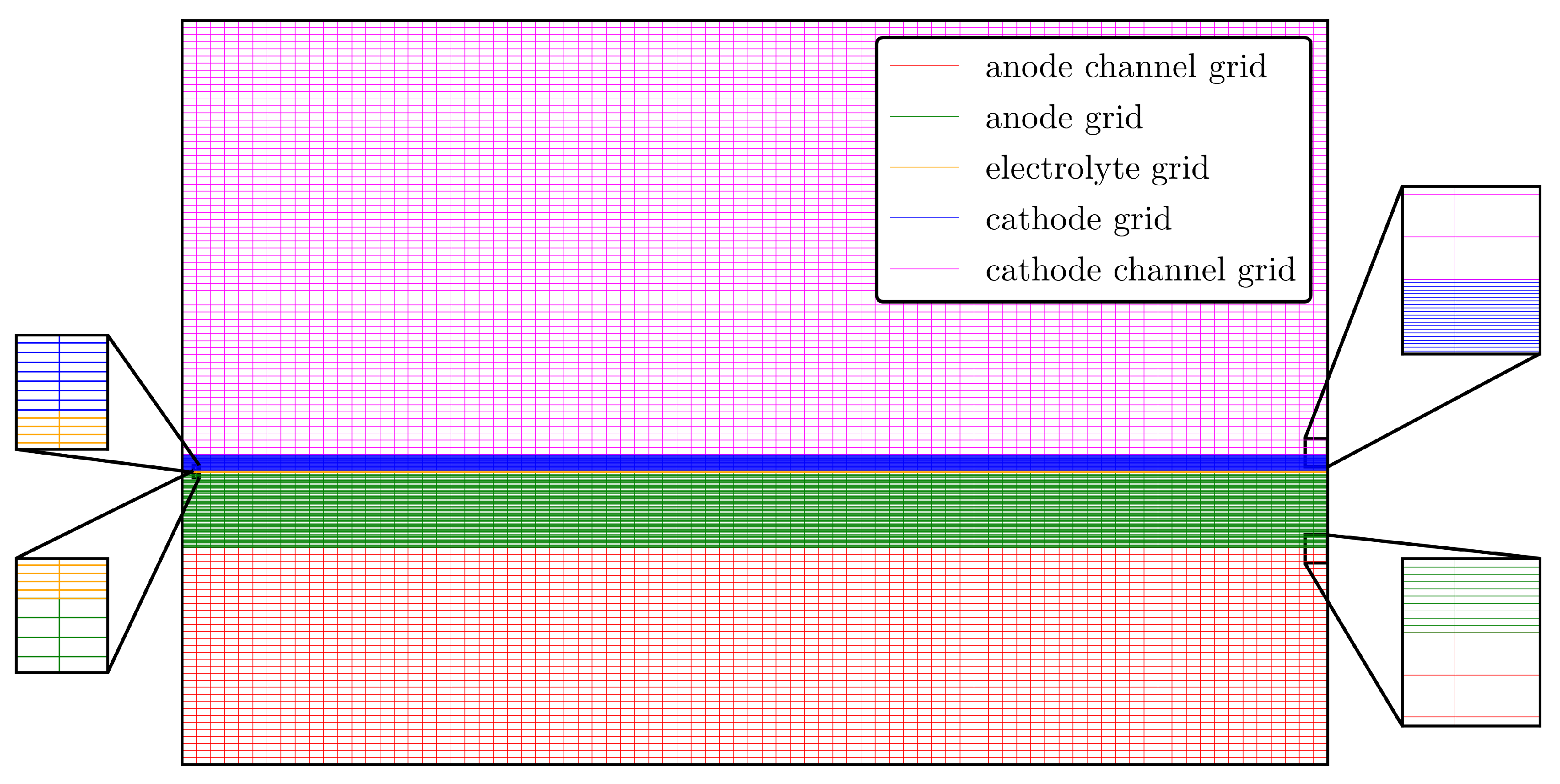
The values of the constants were assumed as $C_1=C_3=10.0$, $C_2=C_4=1.0$. It was found that the relative percent error of the numerical solution is always less than ${10}^{-3}$% for the tests that mimic the simulated system. Based on the results of the MMS, the grid resolution was chosen as follows: in the x-direction, there are 80 control volumes (CVs) and, in the y-direction, there are 60 CVs for the cathode channel, 25 CVs for the cathode, five CVs for the electrolyte, 60 CVs for the anode and 30 CVs for the anode channel.The grid system is shown in Figure 9.

The stop conditions were chosen as follows: for the species transport, the absolute change of the partial pressures between two subsequent iterations should be less than ${10}^{-1}$ $\mathrm{Pa}$; for the energy transport, the absolute change of the temperature between two subsequent iterations should be less than ${10}^{-6}$ $\mathrm{K}$ and, for the charge transport, the absolute change of the potential between two subsequent iterations should be less than ${10}^{-5}$ $\mathrm{V}$. In addition, the relative change of the values of the volumic current density, calculated using the Butler–Volmer model, should be less than 10⁻⁴.

The numerical computations made use of the Prometheus computing cluster, located at AGH University of Science and Technology, Krakow, Poland [76]. A single computational node of the cluster, HP ProLiant XL730f Gen 9 (Hewlett Packard Enterprise, Palo Alto, CA, USA), contains of two $2.5$ $\mathrm{GHz}$ Intel Xeon E5-2680v3 processors (Santa Clara, CA, USA) with 24 cores in total and 128 GB of the RAM memory. The computations were performed on a single node and the time of the computation for a chosen operating voltage was approximately 20 h.

5. Results of the Numerical Computations and Discussion

5.1. Confirmation of the Model

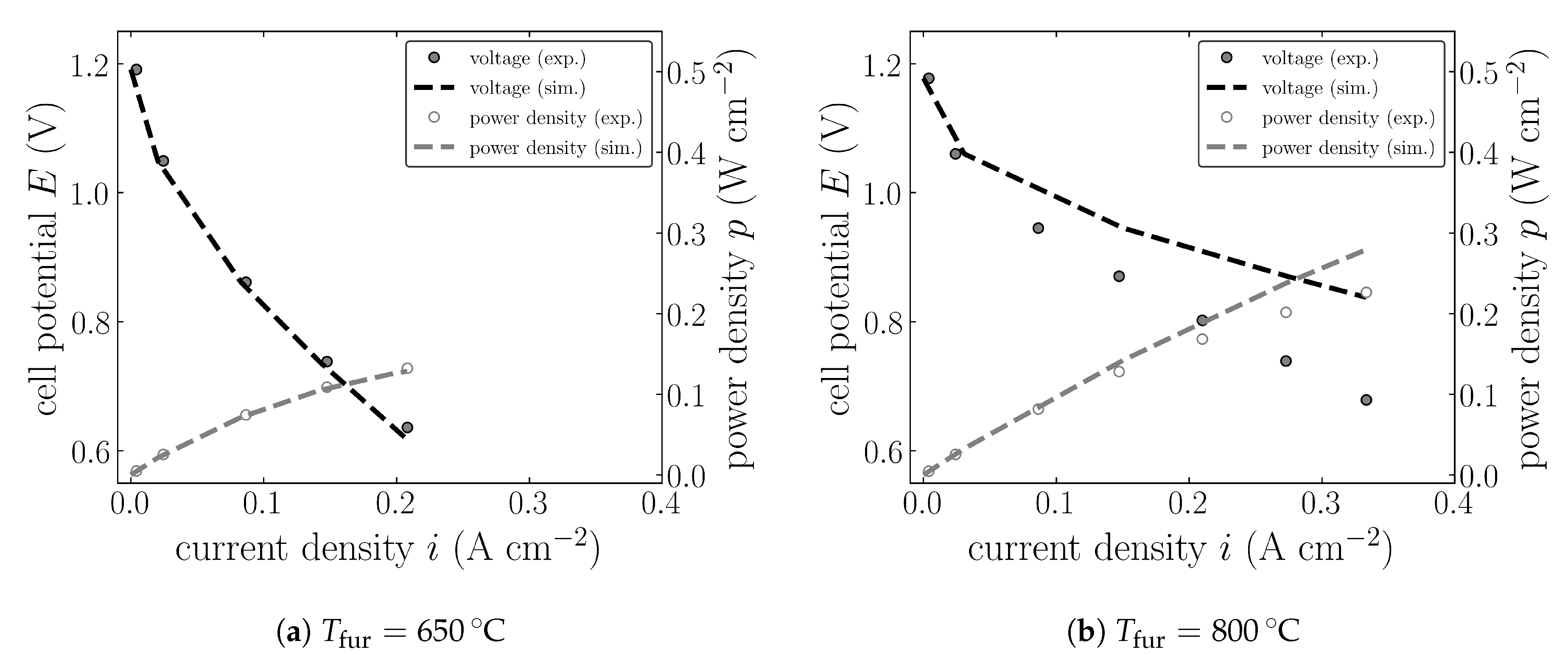
The numerical calculations with the same voltage as in the experimental analysis (see Section 2.2) and with the microstructure the same as the stack (see Section 3) were performed. For the examination of the temperature impact (see Figure 10), the cells which work under 650 ${}^{\circ }\mathrm{C}$ and 800 ${}^{\circ }\mathrm{C}$ (the furnace or wall temperature) were chosen. The fuel composition is 60% of hydrogen and 40% of nitrogen. For the examination of the fuel composition impact, the cells which work under the constant temperature of 750 ${}^{\circ }\mathrm{C}$ (the wall temperature) with the fuel containing 40% of hydrogen and 60% of nitrogen as well as 70% of hydrogen and 30% of nitrogen were chosen. The pressure was set at 101,325 $\mathrm{Pa}$ and the inlet temperature was the same as the wall temperature. The inlet volume flow rates were the same as in the experiment, i.e., $0.28\mathrm{L}{\min }^{-1}$ at the anode channel inlet and $3.2\mathrm{L}{\min }^{-1}$ at the cathode channel inlet (please note that this is the value of the flow rates from Section 2.2 divided by the number of the cells). The cell active area is 48 $\mathrm{cm}$${}^2$. Since in the experiment the dry fuel was used, the amount of water in the fuel is calculated using the Nernst equation from the experimental open circuit voltage (OCV) to simulate the same voltage at zero current conditions. The results are presented in Figure 10 and Figure 11. As can be noticed from Figure 10 and Figure 11, the numerical results are in fair agreement with the experimental data. In Figure 10, it can be observed that, for the cell which works in the lower temperature (650 ${}^{\circ }\mathrm{C}$), the numerical results almost completely overlap with the experimental data (see Figure 10a), whereas the cell which works in 800 ${}^{\circ }\mathrm{C}$ tends to overestimate the performance in the high current density region (Figure 10b). Since for the fuel impact tests the temperature is set at 750 ${}^{\circ }\mathrm{C}$, the cells also overestimate the performance in the high current density region (see Figure 11). Since for safety reasons the current is limited for hydrogen-depleted fuel (the danger of anode oxidation), the effect is especially visible for hydrogen rich fuel (see Figure 11b).

The discrepancy between the numerical and experimental results might be induced by several reasons. The equations for the exchange currents (see Equations (5)) are derived for a cell working under atmospheric pressure, whereas the experiment was conducted under pressurized conditions. The layered structure of the cathode and the presence of the GDC in the cathode are neglected. Nevertheless, the model can correctly predict the trends and qualitative relations.

5.2. Power Generation within the Cell

For the discussion of the current generation, the cell which works under voltage $0.8$ $\mathrm{V}$ or load $0.36$ $\mathrm{A}$ $\mathrm{cm}$${}^2$ was chosen. The wall and inlet temperatures were 750 ${}^{\circ }\mathrm{C}$, the fuel composition was ${\chi }_{{\mathrm{H}}_2}=0.6$ and ${\chi }_{{\mathrm{N}}_2}=0.4$. The total pressure in both channels equals 101,325 $\mathrm{Pa}$. The flow rates were $0.28\mathrm{L}{\min }^{-1}$ at the anode channel inlet and $3.2\mathrm{L}{\min }^{-1}$ at the cathode channel inlet.

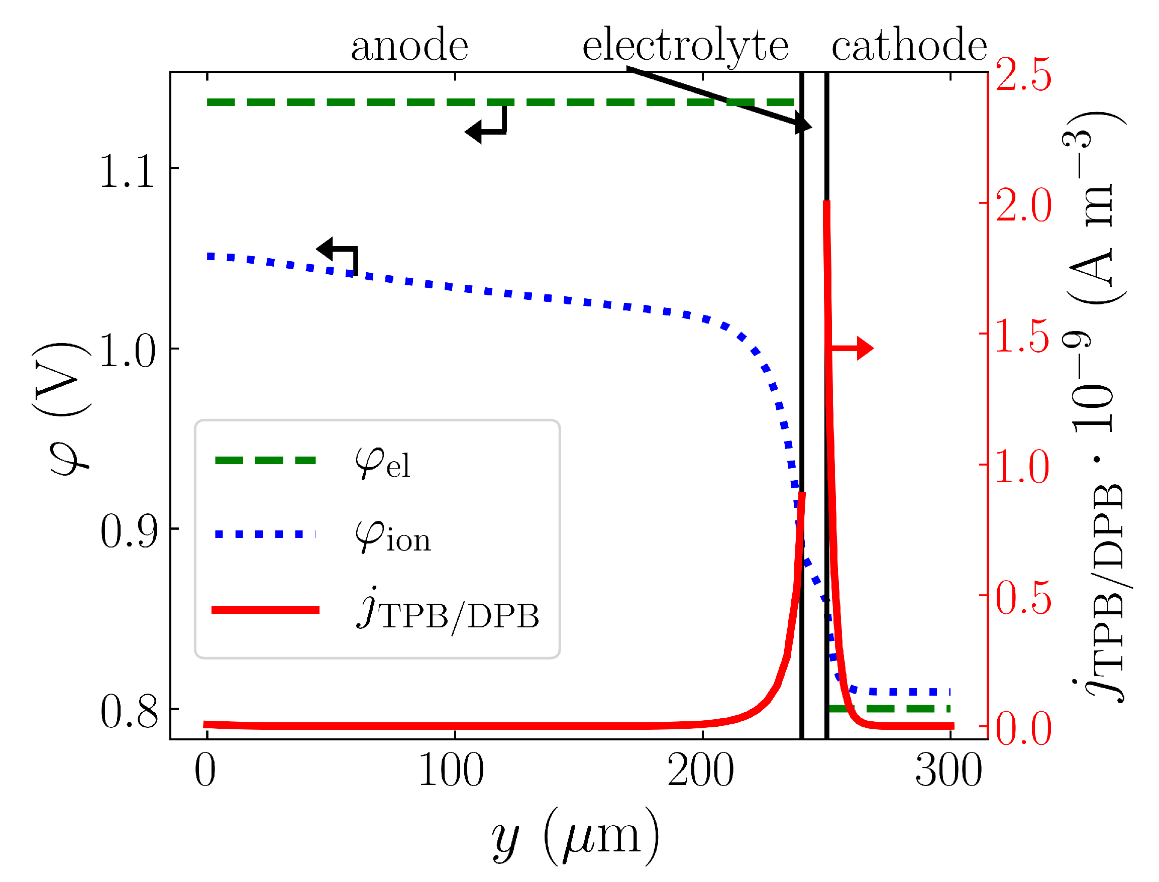
Figure 12 shows the distribution of the averaged potential along the cell depth (the y-direction), as well as the distribution of the averaged volumic current density. The potential of the electron conducting phase is almost constant along the electrode depth, whereas the ionic potential gradually falls from the value similar to the OCV to the value a little bit higher than the operating voltage. As can be noticed, the averaged volumic current density at the TPB and DPB, and the ionic potentials, expect a large change near the interface between the electrodes and electrolyte. Most of the current is produced in this region. This is caused by the fact that the majority of the electrochemical reactions take place near the electrolyte because the mobility of oxygen ions inside the anode and cathode is low.

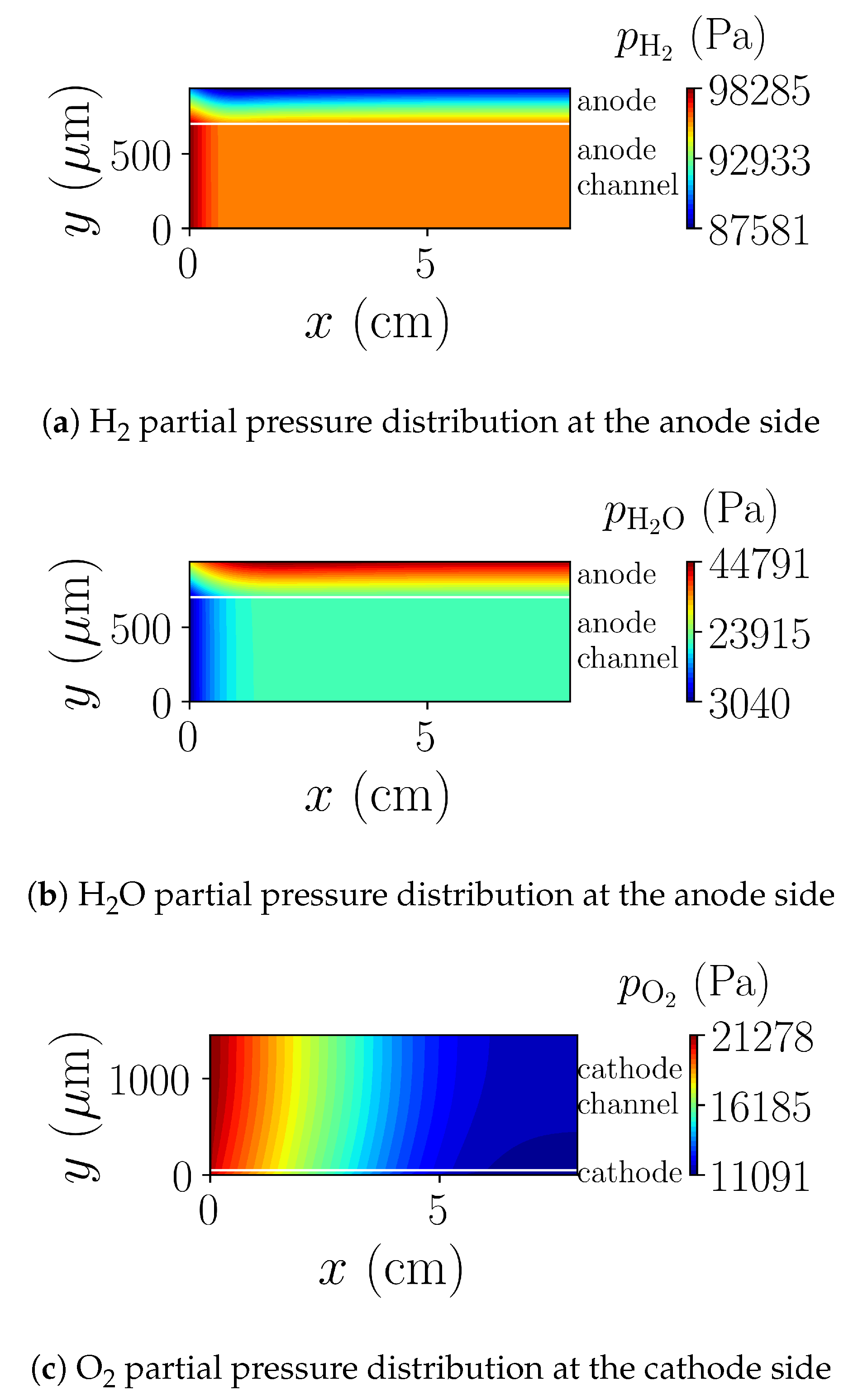
Figure 13a–c show the distribution of the H₂, H₂O and O₂ partial pressures, respectively. As can be observed, at the anode side, a large change occurs near the inlet. However, the fall in hydrogen partial pressure and the water production can be also seen in the electrolyte vicinity in almost all the length of the cell, which is caused by the electrochemical consumption of H₂ and the production of H₂O. The smooth change in the oxygen partial pressure is observed in Figure 13c—the oxygen partial pressure changes almost only in the horizontal direction.

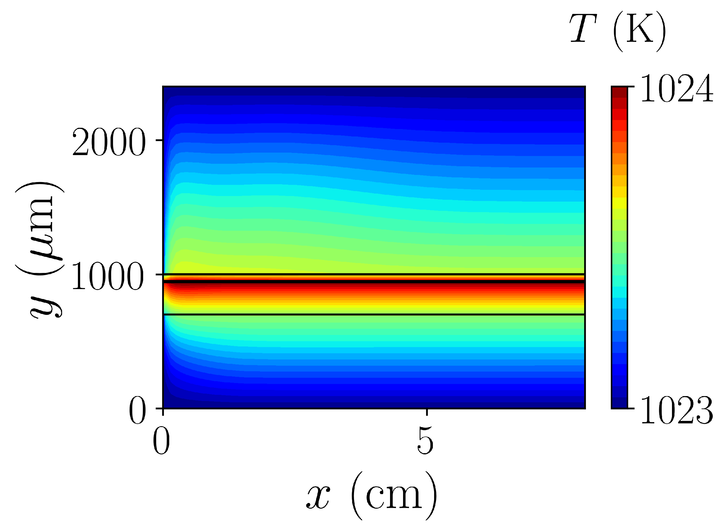
Figure 14 presents the temperature distribution inside the single planar SOFC. The gases are heated near the electrodes, where the source heats are present. However, the overall temperature rise is not significant, about 1 $\mathrm{K}$ and the temperature field is very smooth. This effect may be caused by the thin channels filled with porous material (which enhance the heat transfer) and large inlet temperature (the same as the furnace temperature). In this configuration (the fuel cell enclosed in the constant temperate furnace, which is represented by the Dirichlet boundary conditions on the top and bottom of the system), the cell behaves as an isothermal system. However, this phenomena is desirable, since it prevents against large thermal stresses along the cell.

5.3. Effect of the Microstructure Change

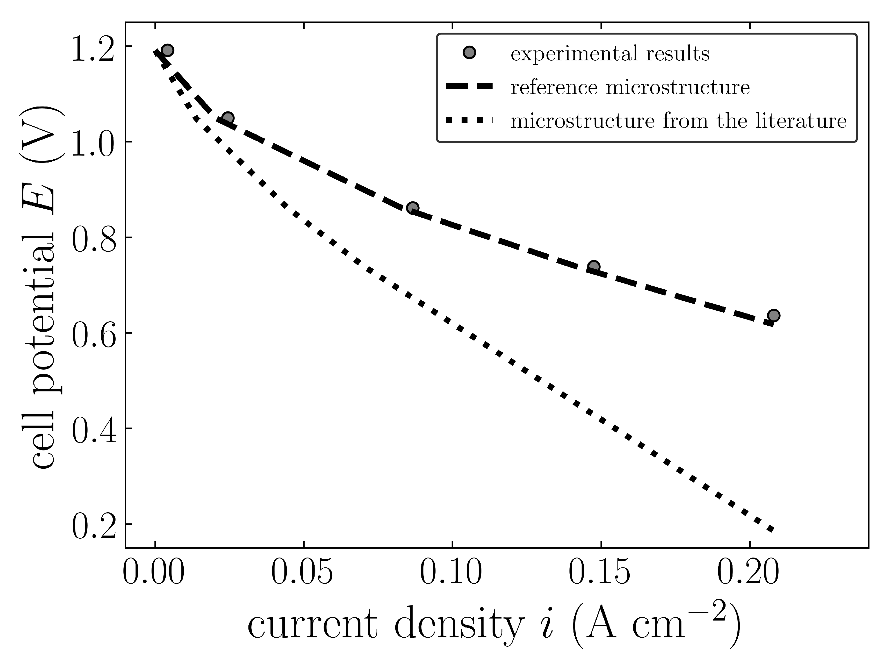
To examine if the microstructure determines the performance of the cell, the different microstructures taken from the literature ([39,41]) serve as an input for the simulation. The summary of both reference and literature microstructure parameters is shown in

Table 13. Reference microstructure for the numerical calculations.

Parameter	Reference Microstructure	Microstructure from the Literature	Literature Reference
${\psi }_{\mathrm{pore},\mathrm{ano}}$	0.26	0.49	[41]
${\psi }_{\mathrm{Ni}}$	0.33	0.26	[41]
${\psi }_{\mathrm{YSZ}}$	0.41	0.25	[41]
${\psi }_{\mathrm{pore},\mathrm{cath}}$	0.39	0.26	[39]
${\psi }_{\mathrm{LSCF}}$	0.61	0.74	[39]
${\tau }_{\mathrm{pore},\mathrm{ano}}$	24.534	1.74	[41]
${\tau }_{\mathrm{Ni}}$	3.647	6.91	[41]
${\tau }_{\mathrm{YSZ}}$	2.240	8.85	[41]
${\tau }_{\mathrm{pore},\mathrm{cath}}$	2.419	2.63	[39]
${\tau }_{\mathrm{LSCF}}$	1.850	2.63	[39]
$d_{\mathrm{pore},\mathrm{ano}}$ ($\mathsf{\mu }\mathrm{m}$)	0.71	0.80	[41]
$d_{\mathrm{pore},\mathrm{cath}}$ ($\mathsf{\mu }\mathrm{m}$)	1.02	0.19	[39]
${\rho }_{\mathrm{TPB},\mathrm{ano}}^L$ ($\mathsf{\mu }\mathrm{m}\mathsf{\mu }{\mathrm{m}}^{-3}$)	4.44	2.43	[41]
${\rho }_{\mathrm{DPB},\mathrm{cath}}^A$ ($\mathsf{\mu }{\mathrm{m}}^2\mathsf{\mu }{\mathrm{m}}^{-3}$)	2.59	3.27	[39]

.

For the computations, the wall and inlet temperatures were 750 ${}^{\circ }\mathrm{C}$. The fuel composition was ${\chi }_{{\mathrm{H}}_2}=0.6$ and ${\chi }_{{\mathrm{N}}_2}=0.4$. The total pressure equals $101.325$ $\mathrm{Pa}$. The flow rates were $0.28\mathrm{L}{\min }^{-1}$ at the anode channel inlet and $3.2\mathrm{L}{\min }^{-1}$ at the cathode channel inlet.

The results of the computations are shown in Figure 15. The results are compared with the experimental data from Section 2.2. As can be observed, when random microstructure is adopted, the model cannot predict the experiment properly. The cell with the microstructure taken from the literature has worse performance compared to the microstructure examined in this study. These results show that the microstructure plays a key role in the SOFC modeling and the multiscale model is necessary to analyze the impact of the microstructure on the cell performance. The inclusion of the microstructure data may increase the quality of the SOFC simulations and open the possibility to optimize the anode and cathode microstructural design.

6. Conclusions

This work shows a multiscale mathematical model of the solid oxide fuel cell. To build the model properly and to gain a set of benchmark data, the experimental investigation of the SOFC short stack and the direct FIB-SEM observation of the porous electrodes have been performed. For the FIB-SEM images segmentation, the semi-automatic algorithm is proposed. Based on the mathematical model, the finite volume numerical model was prepared.

The calculated current–voltage characteristics have been compared to the one obtained from the experiment and a fair agreement was found between the empirical and numerical data. This indicates that the proposed multiscale model can properly predict the electric behavior of a SOFC. The analysis of the current generation inside the cell shows that the current is produced inside the cell primarily near the electrolyte. This effect is connected with a low mobility of the oxygen anions. Furthermore, the simulation of the cell enclosed in a constant temperature furnace, which is represented by the Dirichlet boundary conditions, demonstrates that the SOFC in this case is almost an isothermal system. Calculations with the averaged microstructure parameters adopted from the literature lead to a visible and significant discrepancy between the numerical and experimental data. This confirms that the microstructure has a non-negligible impact on the numerical calculations and should be introduced into the mathematical models of SOFCs.

References

- Molenda, J.; Świerczek, K.; Zajac, W. Functional materials for the IT-SOFC. J. Power Source 2007, 173, 657–670. [Google Scholar] [CrossRef]
- Li, X. Principles of Fuel Cells; Taylor & Francis Group: New York, NY, USA, 2006. [Google Scholar]
- O’Hayre, R.; Cha, S.W.; Colella, W.; Prinz, F.B. Fuel Cell Fundamentals, 3rd ed.; John Wiley & Sons, Inc.: Hoboken, NJ, USA, 2016. [Google Scholar]
- Mozdzierz, M.; Brus, G.; Sciazko, A.; Komatsu, Y.; Kimijima, S.; Szmyd, J.S. An attempt to minimize the temperature gradient along a plug-flow methane/steam reforming reactor by adopting locally controlled heating zones. J. Phys. Conf. Ser. 2014, 530, 1–8. [Google Scholar] [CrossRef]
- Mozdzierz, M.; Brus, G.; Sciazko, A.; Komatsu, Y.; Kimijima, S.; Szmyd, J.S. Towards a Thermal Optimization of a Methane/Steam Reforming Reactor. Flow Turbul. Combust. 2016, 97, 171–189. [Google Scholar] [CrossRef]
- Pajak, M.; Mozdzierz, M.; Chalusiak, M.; Kimijima, S.; Szmyd, J.S.; Brus, G. A numerical analysis of heat and mass transfer processes in a macro-patterned methane/steam reforming reactor. Int. J. Hydrogen Energy 2018, 43, 20474–20487. [Google Scholar] [CrossRef]
- Hidalgo-Vivas, A.; Cooper, B.H. Sulfur removal methods. In Handbook of Fuel Cells—Fundamentals Technology and Applications, Volume 3: Fuel Cell Technology and Applications, Part 1; Vielstich, V., Gasteiger, H.A., Lamm, A., Yokokawa, H., Eds.; John Wiley & Sons, Ltd.: Hoboken, NJ, USA, 2010; pp. 177–189. [Google Scholar]
- Iora, P.; Aguiar, P.; Adjiman, C.S.; Brandon, N.P. Comparison of two IT DIR-SOFC models: Impact of variable thermodynamic, physical, and flow properties. Steady-state and dynamic analysis. Chem. Eng. Sci. 2005, 60, 2963–2975. [Google Scholar] [CrossRef]
- Kleitz, M.; Petitbon, F. Optimized SOFC electrode microstructure. Solid State Ionics 1996, 92, 65–74. [Google Scholar] [CrossRef]
- Sucipta, M.; Kimijima, S.; Suzuki, K. Performance analysis of the SOFC-MGT hybrid system with gasified biomass fuel. J. Power Source 2007, 174, 124–135. [Google Scholar] [CrossRef]
- Salogni, A.; Colonna, P. Modeling of solid oxide fuel cells for dynamic simulations of integrated systems. Appl. Therm. Eng. 2010, 30, 464–477. [Google Scholar] [CrossRef]
- Mozdzierz, M.; Chalusiak, M.; Kimijima, S.; Szmyd, J.S.; Brus, G. An afterburner-powered methane/steam reformer for a solid oxide fuel cells application. Heat Mass Transf. 2018, 54, 2331–2341. [Google Scholar] [CrossRef]
- Recknagle, K.P.; Williford, R.E.; Chick, L.A.; Rector, D.R.; Khaleel, M.A. Three-dimensional thermo-fluid electrochemical modeling of planar SOFC stacks. J. Power Source 2003, 113, 109–114. [Google Scholar] [CrossRef]
- Komatsu, Y.; Kimijima, S.; Szmyd, J.S. Numerical analysis on dynamic behavior of solid oxide fuel cell with power output control scheme. J. Power Source 2013, 223, 232–245. [Google Scholar] [CrossRef]
- Tan, W.C.; Iwai, H.; Kishimoto, M.; Yoshida, H. Quasi-three-dimensional numerical simulation of a solid oxide fuel cell short stack: Effects of flow configurations including air-flow alternation. J. Power Source 2018, 400, 135–146. [Google Scholar] [CrossRef]
- Onaka, H.; Iwai, H.; Kishimoto, M.; Saito, M.; Yoshida, H.; Brus, G.; Szmyd, J.S. Charge-transfer distribution model applicable to stack simulation of solid oxide fuel cells. Heat Mass Transf. 2018, 54, 2425–2432. [Google Scholar] [CrossRef]
- Suzuki, K.; Iwai, H.; Nishino, T. Electrochemical and thermo-fluid modeling of a tubular solid oxide fuel cell with accompanying indirect internal fuel reforming. In Transport Phenomena in Fuel Cells; Sunden, B., Faghri, M., Eds.; WIT Press: Southampton, UK, 2005; pp. 83–131. [Google Scholar]
- Suzuki, M.; Shikazono, N.; Fukagata, K.; Kasagi, N. Numerical analysis of coupled transport and reaction phenomena in an anode-supported flat-tube solid oxide fuel cell. J. Power Source 2008, 180, 29–40. [Google Scholar] [CrossRef]
- Iwai, H.; Yamamoto, Y.; Saito, M.; Yoshida, H. Numerical simulation of intermediate-temperature direct-internal-reforming planar solid oxide fuel cell. Energy 2011, 36, 2225–2234. [Google Scholar] [CrossRef]
- Tan, W.C.; Iwai, H.; Kishimoto, M.; Brus, G.; Szmyd, J.S.; Yoshida, H. Numerical analysis on effect of aspect ratio of planar solid oxide fuel cell fueled with decomposed ammonia. J. Power Source 2018, 384, 367–378. [Google Scholar] [CrossRef]
- Chalusiak, M.; Wrobel, M.; Mozdzierz, M.; Berent, K.; Szmyd, J.S.; Kimijima, S.; Brus, G. A numerical analysis of unsteady transport phenomena in a Direct Internal Reforming Solid Oxide Fuel Cell. Int. J. Heat Mass Transf. 2019, 131, 1032–1051. [Google Scholar] [CrossRef]
- Yakabe, H.; Ogiwara, T.; Hishinuma, M.; Yasuda, I. 3-D model calculation for planar SOFC. J. Power Source 2001, 102, 16–25. [Google Scholar] [CrossRef]
- Milewski, J.; Świrski, K. Modelling the SOFC behaviours by artificial neural network. Int. J. Hydrogen Energy 2009, 34, 5546–5553. [Google Scholar] [CrossRef]
- Chan, S.H.; Xia, Z.T. Anode Micro Model of Solid Oxide Fuel Cell. J. Electrochem. Soc. 2001, 148, A388–A394. [Google Scholar] [CrossRef]
- Prokop, T.A.; Berent, K.; Iwai, H.; Szmyd, J.S.; Brus, G. A three-dimensional heterogeneity analysis of electrochemical energy conversion in SOFC anodes using electron nanotomography and mathematical modeling. Int. J. Hydrogen Energy 2018, 43, 10016–10030. [Google Scholar] [CrossRef]
- Prokop, T.A.; Berent, K.; Szmyd, J.S.; Brus, G. A Three-Dimensional Numerical Assessment of Heterogeneity Impact on a Solid Oxide Fuel Cell’s Anode Performance. Catalysts 2018, 8, 503. [Google Scholar] [CrossRef]
- Suzue, Y.; Shikazono, N.; Kasagi, N. Micro modeling of solid oxide fuel cell anode based on stochastic reconstruction. J. Power Source 2008, 184, 52–59. [Google Scholar] [CrossRef]
- Matsuzaki, K.; Shikazono, N.; Kasagi, N. Three-dimensional numerical analysis of mixed ionic and electronic conducting cathode reconstructed by focused ion beam scanning electron microscope. J. Power Source 2011, 196, 3073–3082. [Google Scholar] [CrossRef]
- He, A.; Gong, J.; Shikazono, N. Three dimensional electrochemical simulation of solid oxide fuel cell cathode based on microstructure reconstructed by marching cubes method. J. Power Source 2018, 385, 91–99. [Google Scholar] [CrossRef]
- Kishimoto, M.; Iwai, H.; Saito, M.; Yoshida, H. Three-Dimensional Simulation of SOFC Anode Polarization Characteristics Based on Sub-Grid Scale Modeling of Microstructure. J. Electrochem. Soc. 2012, 159, B315–B323. [Google Scholar] [CrossRef]
- Jeon, D.H.; Nam, J.H.; Kim, C.J. A random resistor network analysis on anodic performance enhancement of solid oxide fuel cells by penetrating electrolyte structures. J. Power Source 2005, 139, 21–29. [Google Scholar] [CrossRef]
- Yan, Z.; Kim, Y.; Hara, S.; Shikazono, N. Prediction of La0.6Sr0.4Co0.2Fe0.8O3 cathode microstructures during sintering: Kinetic Monte Carlo (KMC) simulations calibrated by artificial neural networks. J. Power Source 2017, 346, 103–112. [Google Scholar] [CrossRef]
- Karakasidis, T.E.; Charitidis, C.A. Multiscale modeling in nanomaterials science. Mater. Sci. Eng. C 2007, 27, 1082–1089. [Google Scholar] [CrossRef]
- Ho, T.X.; Kosinski, P.; Hoffmann, A.C.; Vik, A. Numerical modeling of solid oxide fuel cells. Chem. Eng. Sci. 2008, 63, 5356–5365. [Google Scholar] [CrossRef]
- Sohn, S.; Nam, J.H.; Jeon, D.H.; Kim, C.J. A micro/macroscale model for intermediate temperature solid oxide fuel cells with prescribed fully-developed axial velocity profiles in gas channels. Int. J. Hydrogen Energy 2010, 35, 11890–11907. [Google Scholar] [CrossRef]
- Brus, G.; Iwai, H.; Mozdzierz, M.; Komatsu, Y.; Saito, M.; Yoshida, H.; Szmyd, J.S. Combining structural, electrochemical, and numerical studies to investigate the relation between microstructure and the stack performance. J. Appl. Electrochem. 2017, 47, 979–989. [Google Scholar] [CrossRef]
- Herskovitz, P. A Theoretical Framework For Simulation Validation: Popper’s Falsifications. Int. J. Model. Simul. 1991, 11, 51–55. [Google Scholar] [CrossRef]
- Wilson, J.R.; Kobsiriphat, W.; Mendoza, R.; Chen, H.Y.; Hiller, J.M.; Miller, D.J.; Thornton, K.; Voorhees, P.W.; Adler, S.B.; Barnett, S.A. Three-dimensional reconstruction of a solid-oxide fuel-cell anode. Nat. Mater. 2006, 5, 541–544. [Google Scholar] [CrossRef] [PubMed]
- Gostovic, D.; Smith, J.R.; Kundinger, D.P.; Jones, K.S.; Wachsman, E.D. Three-Dimensional Reconstruction of Porous LSCF Cathodes. Electrochem. Solid-State Lett. 2007, 10, B214–B217. [Google Scholar] [CrossRef]
- Iwai, H.; Shikazono, N.; Matsui, T.; Teshima, H.; Kishimoto, M.; Kishida, R.; Hayashi, D.; Matsuzaki, K.; Kanno, D.; Saito, M.; et al. Quantification of SOFC anode microstructure based on dual beam FIB-SEM technique. J. Power Source 2010, 195, 955–961. [Google Scholar] [CrossRef]
- Kishimoto, M.; Iwai, H.; Saito, M.; Yoshida, H. Quantitative evaluation of solid oxide fuel cell porous anode microstructure based on focused ion beam and scanning electron microscope technique and prediction of anode overpotentials. J. Power Source 2011, 196, 4555–4563. [Google Scholar] [CrossRef]
- Schindelin, J.; Arganda-Carreras, I.; Frise, E.; Kaynig, V.; Longair, M.; Pietzsch, T.; Preibisch, S.; Rueden, C.; Saalfeld, S.; Schmid, B.; et al. Fiji: An open-source platform for biological-image analysis. Nat. Methods 2012, 9, 676–682. [Google Scholar] [CrossRef]
- Rueden, C.T.; Schindelin, J.; Hiner, M.C.; DeZonia, B.E.; Walter, A.E.; Arena, E.T.; Eliceiri, K.W. ImageJ2: ImageJ for the next generation of scientific image data. BMC Bioinform. 2017, 18, 1–26. [Google Scholar] [CrossRef]
- van der Walt, S.; Schonberger, J.L.; Nunez-Iglesias, J.; Boulogne, F.; Warner, J.D.; Yager, N.; Gouillart, E.; Yu, T. scikit-image: Image processing in Python. PeerJ 2014, 2, 1–18. [Google Scholar] [CrossRef]
- Oppenheim, A.V.; Schafer, R.W.; Stockham, T.G. Nonlinear Filtering of Multiplied and Convolved Signals. Proc. IEEE 1968, 56, 1264–1291. [Google Scholar] [CrossRef]
- Nock, R.; Nielsen, F. Statistical Region Merging. IEEE Trans. Pattern Anal. Mach. Intell. 2004, 26, 1452–1458. [Google Scholar] [CrossRef]
- Arganda-Carreras, I.; Kaynig, V.; Rueden, C.; Eliceiri, K.W.; Schindelin, J.; Cardona, A.; Seung, H.S. Trainable Weka Segmentation: A machine learning tool for microscopy pixel classification. Bioinformatics 2017, 33, 2424–2426. [Google Scholar] [CrossRef]
- Lee, J.H.; Moon, H.; Lee, H.W.; Kim, J.; Kim, J.D.; Yoon, K.H. Quantitative analysis of microstructure and its related electrical property of SOFC anode, Ni-YSZ cermet. Solid State Ionics 2002, 148, 15–26. [Google Scholar] [CrossRef]
- Nakashima, Y.; Kamiya, S. Mathematica Programs for the Analysis of Three-Dimensional Pore Connectivity and Anisotropic Tortuosity of Porous Rocks using X-ray Computed Tomography Image Data. J. Nucl. Sci. Technol. 2007, 44, 1233–1247. [Google Scholar] [CrossRef]
- Esquirol, A.; Kilner, J.; Brandon, N. Oxygen transport in La0.6Sr0.4Co0.2Fe0.8O3−δ/Ce0.8Ge0.2O2−x composite cathode for IT-SOFCs. Solid State Ionics 2004, 175, 63–67. [Google Scholar] [CrossRef]
- de Boer, B. SOFC Anode: Hydrogen Oxidation at Porous nickel and nickel/yttria stabilised zirconia cermet electrodes. Ph.D Thesis, Twente University, Enschede, The Netherlands, 9 October 1998. [Google Scholar]
- Fleig, J.; Baumann, F.S.; Maier, J. The Oxygen Reduction Kinetics of Mixed Conducting Electrodes: Model Considerations and Experiments on La0.6Sr0.4Co0.8Fe0.2O3 Microelectrodes. Proc. Electrochem. Soc. 2005, 2005-07, 1636–1644. [Google Scholar] [CrossRef]
- Esquirol, A.; Brandon, N.P.; Kilner, J.A.; Mogensen, M. Electrochemical Characterization of La0.6Sr0.4Co0.2Fe0.8O3 Cathodes for Intermediate-Temperature SOFCs. J. Electrochem. Soc. 2004, 151, A1847–A1885. [Google Scholar] [CrossRef]
- Nield, D.A.; Bejan, A. Convection in Porous Media, 4th ed.; Springer Science+Business Media: New York, NY, USA, 2013. [Google Scholar]
- Bear, J. Dynamics of Fluids in Porous Media; Dover Publications, Inc.: New York, NY, USA, 1972. [Google Scholar]
- Suwanwarangkul, R.; Croiset, E.; Fowler, M.W.; Douglas, P.L.; Entchev, E.; Douglas, M.A. Performance comparison of Fick’s, dusty-gas and Stefan-Maxwell models to predict the concentration overpotential of a SOFC anode. J. Power Source 2003, 122, 9–18. [Google Scholar] [CrossRef]
- Yakabe, H.; Hishinuma, M.; Uratani, M.; Matsuzaki, Y.; Yasuda, I. Evaluation and modeling of performance of anode-supported solid oxide fuel cell. J. Power Source 2000, 86, 423–431. [Google Scholar] [CrossRef]
- Poling, B.E.; Prausnitz, J.M.; O’Connell, J.P. The Properties of Gases and Liquids, 5th ed.; McGraw-Hill: New York, NY, USA, 2001. [Google Scholar]
- Fuller, E.N.; Schettler, P.D.; Giddings, J.C. A New Method for Prediction of Binary Gas-Phase Diffusion Coefficients. Ind. Eng. Chem. 1966, 58, 18–27. [Google Scholar] [CrossRef]
- Todd, B.; Young, J. Thermodynamic and transport properties of gases for use in solid oxide fuel cell modelling. J. Power Source 2002, 110, 186–200. [Google Scholar] [CrossRef]
- Mason, E.A.; Saxena, S.C. Approximate Formula for the Thermal Conductivity of Gas Mixtures. Phys. Fluids 1958, 1, 361. [Google Scholar] [CrossRef]
- Roy, D.; Thodos, G. Thermal Conductivity of Gases. I&EC Fundam. 1968, 7, 529–534. [Google Scholar]
- Roy, D.; Thodos, G. Thermal Conductivity of Gases Organic Compounds at Atmospheric Pressure. I&EC Fundam. 1970, 9, 71–79. [Google Scholar]
- Funahashi, Y.; Shimamori, T.; Suzuki, T.; Fujishiro, Y.; Awano, M. Simulation Study for the Optimization of Microtubular Solid Oxide Fuel Cell Bundles. J. Fuel Cell Sci. Technol. 2010, 7, 021015–1–021015–4. [Google Scholar] [CrossRef]
- Schlichting, K.W.; Padture, N.P.; Klemens, P.G. Thermal conductivity of dense and porous yttria-stabilized zirconia. J. Mater. Sci. 2001, 36, 3003–3010. [Google Scholar] [CrossRef]
- Iwata, M.; Hikosaka, T.; Morita, M.; Iwanari, T.; Ito, K.; Onda, K.; Esaki, Y.; Sakaki, Y.; Nagata, S. Performance analysis of planar-type unit SOFC considering current and temperature distributions. Solid State Ionics 2000, 132, 297–308. [Google Scholar] [CrossRef]
- Graves, R.S.; Kollie, T.G.; McElroy, D.L.; Gilchrist, K.E. The thermal conductivity of AISI 304L stainless steel. Int. J. Thermophys. 1991, 12, 409–415. [Google Scholar] [CrossRef]
- Anselmi-Tamburini, U.; Chiodelli, G.; Arimondi, M.; Maglia, F.; Spinolo, G.; Munir, Z.A. Electrical properties of Ni/YSZ cermets obtained through combustion synthesis. Solid State Ionics 1998, 110, 35–43. [Google Scholar] [CrossRef]
- Gong, J.; Li, Y.; Tang, Z.; Xie, Y.; Zhang, Z. Temperature-dependence of the lattice conductivity of mixed calcia/yttria-stabilized zirconia. Mater. Chem. Phys. 2002, 76, 212–216. [Google Scholar] [CrossRef]
- Bouwmeester, H.J.M.; Den Otter, M.W.; Boukamp, B.A. Oxygen transport in La0.6Sr0.4Co1−yFeyO3−δ. J. Solid State Electrochem. 2004, 8, 599–605. [Google Scholar] [CrossRef]
- Jones, E.; Oliphant, T.; Peterson, P. SciPy: Open Source Scientific Tools for Python. Available online: https://www.scipy.org/ (accessed on 11 March 2019).
- Patankar, S.V. Numerical Heat Transfer and Fluid Flow; Hemisphere Publishing Corporation: Washington, DC, USA, 1980. [Google Scholar]
- Moukalled, F.; Mangani, L.; Darwish, M. The Finite Volume Method in Computational Fluid Dynamics: An Advanced Introduction with OpenFOAM and Matlab; Springer International Publishing: Cham, Switzerland, 2016. [Google Scholar]
- van der Vorst, H. Bi-CGSTAB: A fast and smoothly converging variant of Bi-CG for the solution of nonsymmetric linear systems. SIAM J. Sci. Stat. Comp. 1992, 13, 631–644. [Google Scholar] [CrossRef]
- Roache, P.J. Code Verification by the Method of Manufactured Solutions. J. Fluids Eng. 2002, 124, 4–10. [Google Scholar] [CrossRef]
- Prometheus. Available online: https://kdm.cyfronet.pl/portal/Prometheus (accessed on 1 March 2019).
Figure 1.
Principle of the solid oxide fuel cell operation.
Figure 2.
Configuration of the modular stack test bench.
Figure 3.
Experimental results. (a) current–voltage and current–power characteristics in the different furnace temperatures; (b) current–voltage and current–power characteristics for the different fuel mixtures.
Figure 4.
Configuration of the FEI Versa 3D FIB-SEM apparatus.
Figure 5.
Semi-automatic segmentation procedure, on the example of the cathode FIB-SEM image.
Figure 6.
Segmentation of the FIB-SEM images.
Figure 7.
Three-dimensional reconstruction of the anode and cathode.
Figure 8.
Computational domain for the SOFC simulations.
Figure 9.
The grid system used for the computations.
Figure 10.
Comparison of the experimental and numerical data for the different furnace temperatures (, ).
Figure 11.
Comparison of the experimental and numerical data for the different inlet fuel compositions ().
Figure 12.
Distribution of the averaged electronic and ionic potentials, and the average volumic current density in cell depth direction.
Figure 13.
Partial pressure distribution inside the system (not in the scale).
Figure 14.
Temperature distribution inside the cell (not in the scale); the cathode channel is on the top.
Figure 15.
Comparison of the computations with two different microstructure parameters with the experimental results for , , .