Article

Cancer-Cell Deep-Learning Classification by Integrating Quantitative-Phase Spatial and Temporal Fluctuations

Department of Biomedical Engineering, Tel Aviv University, Tel Aviv 6997801, Israel
*
Author to whom correspondence should be addressed.
Submission received: 30 October 2021 / Revised: 23 November 2021 / Accepted: 25 November 2021 / Published: 29 November 2021
(This article belongs to the Special Issue Current Trends in Quantitative Phase Imaging of Cells and Tissues)

Abstract

:
We present a new classification approach for live cells, integrating together the spatial and temporal fluctuation maps and the quantitative optical thickness map of the cell, as acquired by common-path quantitative-phase dynamic imaging and processed with a deep-learning framework. We demonstrate this approach by classifying between two types of cancer cell lines of different metastatic potential originating from the same patient. It is based on the fact that both the cancer-cell morphology and its mechanical properties, as indicated by the cell temporal and spatial fluctuations, change over the disease progression. We tested different fusion methods for inputting both the morphological optical thickness maps and the coinciding spatio-temporal fluctuation maps of the cells to the classifying network framework. We show that the proposed integrated triple-path deep-learning architecture improves over deep-learning classification that is based only on the cell morphological evaluation via its quantitative optical thickness map, demonstrating the benefit in the acquisition of the cells over time and in extracting their spatio-temporal fluctuation maps, to be used as an input to the classifying deep neural network.

1. Introduction

The classification of cancerous cells is an important medical endeavor of great significance for biophysical assays and medical diagnoses. Attempts to compare healthy cells to cancerous cells have been made for years, and numerous biomarkers have been discovered to distinguish between them. Most of these biomarkers are based on using exogenous cell labeling, which requires prior knowledge of the labeling agent. Alternatively, label-free measurements of the intrinsic properties of the cells for cell discrimination can be used. One of the important label-free biomarkers is cell stiffness, which is associated with disease invasiveness [1,2,3,4,5,6]. Most studies have shown that metastatic cancer cells, which have been detached from the tumor, are less stiff and have a higher migratory and invasive potential than primary tumor cells.
A popular method for determining cell stiffness is by using atomic force microscopy (AFM) [3,4,5,6]. However, this approach is complicated, slow, expensive, and difficult to execute in clinics. Other techniques, such as micropipette aspiration, optical tweezers, and magnetic twisting cytometry [7,8], also show a substantial inverse correlation between cancer-cell stiffness and metastatic potential. However, these methods are cell invasive and may lead to cell damage.
Non-invasive techniques, such as interferometric phase microscopy (IPM), can record holographic images of biological cells. These images provide the dynamic optical path delay (OPD) topographic maps of the cells without the use of cell staining [9,10,11]. We have previously shown that various morphological and textural parameters derived directly from the cell OPD maps, including the cell dry mass and phase volume, can be used to obtain statistical differences between healthy and different cancer cells [12]. The OPD temporal fluctuations can be used as an indicative analysis tool (e.g., [13,14]). Specifically, the mean standard deviation of the cell temporal fluctuations, as extracted from the cell OPD profile over time, can be used to obtain statistical differences between healthy and different cancer cells [15]. The cell fluctuations are indicative of the cell stiffness, where cancer cells change their stiffness as cancer progresses, in addition to their three-dimensional (3D) morphology. Furthermore, the OPD map can be used to calculate the cell spatial fluctuations, which are the basis for the cell disorder strength, a parameter that is also linked to cell stiffness [16,17]. Thus, both the morphology and the spatio-temporal fluctuations should be taken into account when evaluating the cell metastatic potential.
Previous studies have used simple machine-learning classifiers on cell OPD maps to discriminate between various cellular conditions (e.g., [12,18]). With advances in deep learning, other studies have distinguished between the invasiveness levels of cancer cells. Most of them used only the OPD-based morphology of the cell (e.g., [19,20]). Deep-learning classifiers based on temporal fluctuations have been previously used to classify red blood cells [21] and SARS-CoV-2 virus particles [22].
Here we present a new method that uses the cell temporal fluctuations, on top of the cell spatial fluctuations and morphology, as the basis for cancer-cell classification. This requires capturing a video of the OPD maps of the cells and extracting the temporal and spatial fluctuations as an input for the classifier. The fact that we now have very different domains characterizing the cells, the morphological OPD domain and the spatio-temporal fluctuations domain gives rise to the question of how to fuse them into the classifying network architecture. This is going to be explored as well.
In general, the use of deep learning to classify videos involves methods such as 3D convolutional neural networks (CNN), optical flow computation, and long short-term memory (LSTM) networks [21,23,24,25]. These methods would fail to capture extremely minor changes for hundreds of frames, which is needed for quantifying cancer cell fluctuations. Our approach, on the other hand, extracts both the spatial and temporal fluctuations from the video as one image per cell, and utilizes a unique triple-path neural-network architecture to integrate the cell morphology and cell fluctuations, and use them for cell classification.

2. Materials and Methods

2.1. Dataset

Our dataset contains 216 videos of live colorectal adenocarcinoma cancer cells. Each video contains a single cell. The primary colon cancer cells (from SW480 cell line) contained 104 videos, whereas the metastatic colon cancer cells (from SW620 cell line) contained 112 videos. Both cell lines were purchased from the ATCC and originated from the same patient. Each video was recorded for 4 s at a rate of 500 frames/sec with a resolution of 512 × 512 pixels.

2.2. Cell Preparation and Imaging

The cells were grown in a Dulbecco’s Modified Eagle Medium (DMEM) until 80% confluence, and then trypsinized to suspend them. The optical system used to acquire the cells is presented in Figure 1. This system is based on diffraction phase microscopy (DPM) [26]. A commercial microscope (IX83, Olympus) was illuminated by a low-coherence laser beam (SuperK Extreme, NKT) connected to an acousto-optical tunable filter, creating a wavelength bandwidth of 633 ± 2.5 nm. The sample passed through the cell sample and was magnified by a 40× microscope objective and projected by a tube lens onto the microscope output plane, where a custom-built DPM module was located. This is an external common-path interferometric module that creates an off-axis hologram on the camera. This is done by using a diffraction grating to split the sample image into two beams and erasing the sample information from one of the beams using spatial filtering, effectively turning it into a reference beam. The spatial filtering is implemented by a 4f lens configuration, and a pinhole located at the confocal plane. Another 4f lens configuration creates a secondary magnification of 6×. The off-axis hologram is captured by a fast camera (Photron FASTCAM Mini AX200).
We extracted the optical path delay (OPD) from each of the recorded off-axis holograms using the digital procedure described in [27,28], including a Fourier transform cropping one of the cross-correlation terms, an inverse Fourier transform, two-dimensional phase unwrapping on the phase argument, and a division by 2 π / λ , where λ is the central illumination wavelength. Then, each OPD video per cell is resized to 250 × 250 pixels. Examples of the resulting cell OPD maps are presented in Figure 2.

2.3. Pre-Processing Technique

Regular approaches for classifying videos in deep learning aim to capture substantial displacement in space, such as throwing a ball. In our case, we have to capture subtle OPD fluctuations in cancer cells, so those methods would fail. In addition, we need to deal with a large amount of data (2000 frames for each cell), while capturing the essence of the movements.
To solve this issue, and capture both spatial and temporal frequencies from the video in one image per cell, we used the representation suggested by Popescu et al. [29]. First, we excluded the edges of the cell due to increased vibrations in these areas. For this, we created a mask, based on the first image from each video, and applied this mask to the whole video (see Figure 3a,d). Figure 3b,e present the temporal-fluctuation standard deviation maps obtained. In the following step, for each frame from each video representing one cell in the database, we subtracted the average frame, and calculated the Fourier transform in three dimensions. Then, for each temporal frequency, we calculated the radially averaged power spectral density and built a fluctuation map with two axes: the horizontal axis represents spatial frequencies q, and the vertical axis represents temporal frequencies ω (see Figure 3c,f). Figure 3g shows a histogram of the mean OPD value on the cell area for the two groups of cells, demonstrating that there is a statistical difference between the groups with p < 0.0005, but without full seperation. Figure 3h shows a histogram of the mean of the absolute values of the spatio-temporal fluctuation map, demonstrating again that there is a statistical difference between the groups with p < 0.0005, but without full seperation. These results support the development of an automatic classifier on a cell-by-cell basis that takes into consideration both the OPD and the spatio-temporal fluctuations.

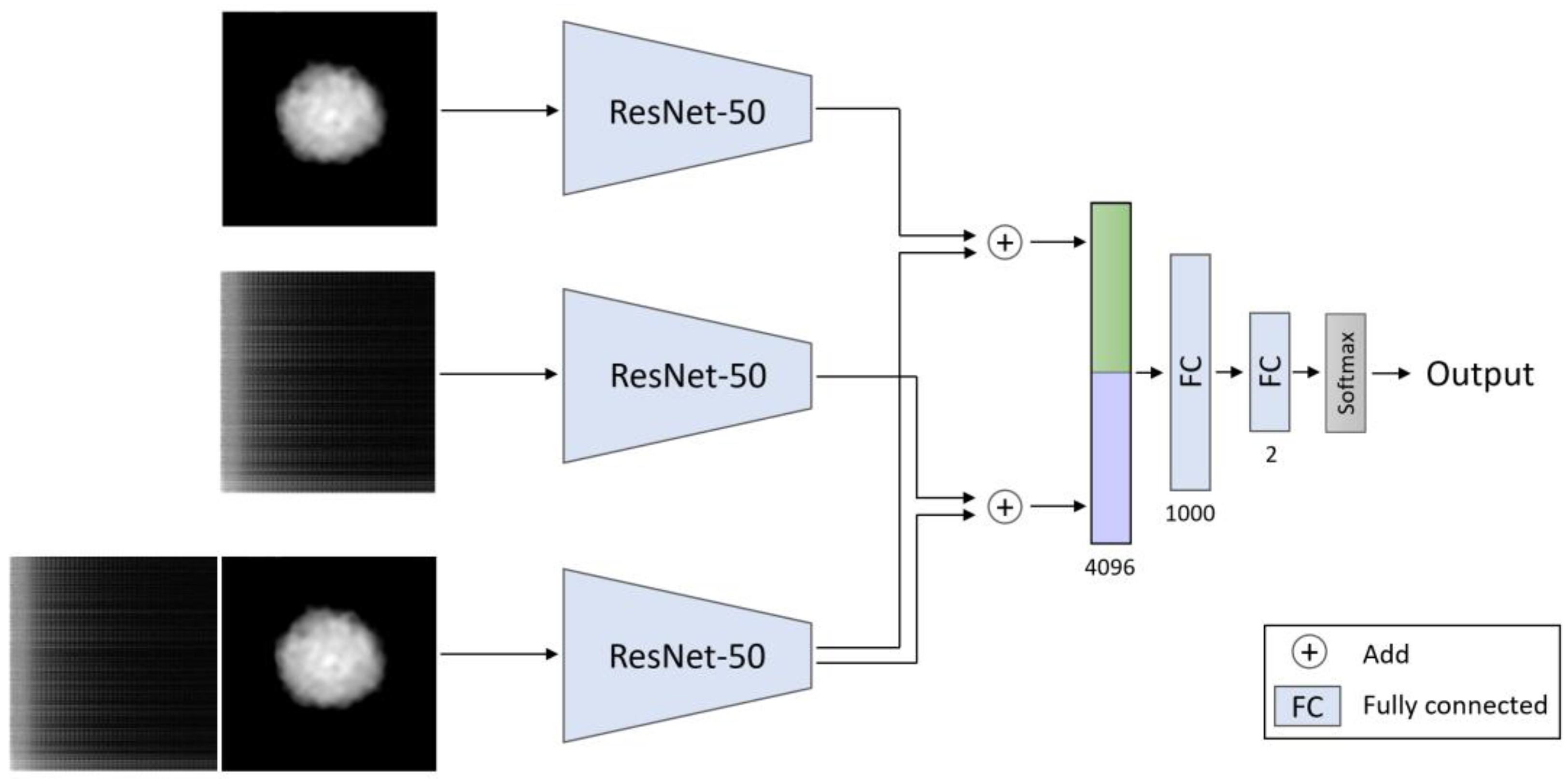
2.4. Framework for Deep-Learning-Based Classification

We selected the ResNet-50 architecture [30], pre-trained on ImageNet [31], to distinguish between primary cells and metastatic cells. Some CNNs may suffer from low diagnostic performance due to the vanishing-gradient and the divergence-gradient problems, which obstruct information transmission from shallow layers to deep layers of the network. ResNet-50 solves this problem by identifying shortcut connections, skipping certain layers while providing great generalization performance with a relatively small number of parameters. Indeed, ResNet-50 has been successfully used for many medical image classification tasks [32]. We therefore selected it for our case as well.
We trained this network for each modality separately: (1) the cell stationary morphology (OPD) maps, which formed our baseline model; and (2) the spatio-temporal fluctuation maps described in Section 2.3. Each architecture learns from each modality a specific structure, and can thus lead to better classification results by integrating both modalities. Based on this assumption, we created a multimodal network and used early- and late-fusion techniques [33] to combine the features, as described next.
First, we examined the early-fusion technique, which involves integration between the two modalities before being used as an input to the network. We concatenated each modality (the cell morphology map or the spatio-temporal fluctuation map) across the channel dimension and trained a simple ResNet architecture.
Then, we examined the late-fusion technique, which involves the aggregation of decisions from multiple networks, and created a double-path model (see Figure 4). We employed a modified ResNet-50 architecture in each path, removing the last two layers (softmax and fully connected layers) and flattening the output of the average pooling layer. Then, we inserted the cell morphology map or the fluctuation map for each path respectively, thus creating a feature vector for each modality. We used the late-fusion approach and concatenated each feature vector from each modality and passed the unified vector to a classifier.
To achieve better performance, we developed a new model with a triple path, as presented in Figure 5. This model combines the advantage of the early-fusion technique, which is the automatic learning of the cross-modal representation, with the advantage of the late-fusion technique, enhancing the features of the different modalities by two independent modules. We employed the same modified ResNet-50 architecture and inserted three inputs: (1) the cell morphology map; (2) the spatio-temporal fluctuation map; (3) a two-channel input that concatenated between the cell morphology and the spatio-temporal fluctuation maps. We extracted a feature vector from each path and added the two-channel feature vector to the cell-morphology feature vector and to the spatio-temporal-fluctuation-map feature vector. Then, we concatenated those two vectors and passed the unified vector to a classifier.

2.5. Implementation Details

All models were trained using the cross-entropy (CE) loss with a batch size of 8, a learning rate of 2 × 10⁻⁶, and an ADAM optimizer. To improve generalization, we randomly created 20 different shuffles. Each shuffle was split into train, validation, and test sets (60%, 20%, 20%), and the epoch with the highest score on the validation set was chosen for the test set. Each shuffle was trained for 100 epochs. The reported results are obtained from the mean and standard deviation (std) across all the shuffles.

3. Results

To evaluate the various methods, we used five different measurements: accuracy, sensitivity, specificity, precision, and area under curve (AUC). The results are presented in Table 1. We examined all the different architectures: single-path ResNet, double-path ResNet and triple-path ResNet. We also compared between early and late-fusion techniques by employing different inputs: the morphology, the spatio-temporal fluctuation map and/or the two-channel input, as described in Section 2.4. As presented in Table 1, combining the morphology and spatio-temporal fluctuation map (triple-path model) improves the results from 85% (morphology only) to 89% (combining morphology and spatio-temporal fluctuations).
Figure 6 shows the shuffle-averaged accuracy and loss of the chosen triple-path model, indicating that no overfitting occurs.

4. Discussion and Conclusions

In this work, we presented a new approach for classifying cancer cells based on the cell spatial and temporal fluctuations, in addition to the cell OPD-based morphology. We demonstrated that by using a 3D Fourier transform on the fluctuations, we can extract a single map per cell, quantifying the subtle spatio-temporal fluctuations of the cell. We also demonstrated that by using a smart integration of the OPD-based morphology and fluctuation maps of cancer cells, improved classification performance is obtained, compared to classifying according to the OPD-based morphology alone. Our approach to integration combines various fusion techniques. The early-fusion technique, also known as feature-level fusion, combines the modalities before they are input into the network, resulting in a single feature vector for both modalities. The late-fusion technique, also known as decision-level fusion, first fuses the feature vector for each modality, then merges the vectors and sends the resulting single vector to a classifier. We can see from the results that using both fusion approaches together in the triple-path model yields the best performance.
Note that the cells of the two groups were imaged in several different dishes, prepared together under the same conditions. This procedure minimizes possible differences between dishes. Furthermore, since the collection of each group of cells was done in five different dishes, differences between dishes that might have caused changes between the groups weres further minimized. Thus, the classifier did not learn the difference between the dishes, but between the groups of cells.
Previous approaches [12] used handcrafted features extracted from the cancer cell morphological OPD map to train a simple classifier instead of using the cell OPD map directly, without feature extraction, to train a deep-learning classifier. When classifying between SW420 and SW620 cells, the same cells as analyzed in the current paper, 82% sensitivity, 81% specificity, and 89.7% AUC were obtained. Note that the results presented in Table 1 are better, even for the case of the OPD morphology map representation alone, with 82.38% sensitivity, 88.17% specificity, and 93.66% AUC. Even stronger results are achieved when analyzing the cells based on both the OPD morphology map and the spatio-temporal fluctuation map by the proposed triple-path model, yielding 88.89% sensitivity, 89.32% specificity, and 96.03% AUC. These results demonstrate the usefulness of the proposed deep-learning framework that classifies the cell OPD map and the fluctuation map at the pixel level, and does not need to rely on extracting specific handcrafted features prior to the cell classification task.
With the introduction of portable and easy-to-use interferometric modules [34,35], which are suitable for direct clinical use, the proposed cancer-cell classification method can be utilized for cancer diagnosis in medical clinics, for detection and monitoring of circulating tumor cells isolated from liquid biopsies [36,37], such as blood, as well as for analyzing cancer cells extracted from solid tumors and tissue biopsies. For these clinical applications, correlating the cell metastatic potential with its OPD morphology and spatio-temporal fluctuation maps is of utmost importance, since it can help in diagnosing and monitoring the patient’s disease stage, and define the suitable therapeutic paths. Our method also forms a general analysis and classification approach for red blood cells, as well as other types of cells expressing stiffness changes.

Author Contributions

Conceptualization, N.T.S.; Investigation, S.B.B., N.R.-N., N.T.S.; Methodology, S.B.B., N.R.-N., A.B., H.G., N.T.S.; Resources, N.T.S., H.G.; Software, S.B.B., N.R.-N.; Supervision, N.T.S., H.G.; Visualization, S.B.B.; Writing—original draft, S.B.B., N.T.S.; Writing—review & editing, H.G., N.R.-N.; Funding acquisition, N.T.S., H.G. All authors have read and agreed to the published version of the manuscript.

Funding

Horizon 2020 ERC grant (678316) (S.B.B., N.N.-R., N.T.S.). Grant from the Israeli Ministry of Science & Technology (3-16467) (A.B., H.G.).

Institutional Review Board Statement

Not applicable.

Informed Consent Statement

Not applicable.

Data Availability Statement

Additional data can be obtained upon a reasonable request.

Conflicts of Interest

The authors declare no conflict of interest.

References

  1. Cross, S.E.; Jin, Y.S.; Rao, J.; Gimzewski, J.K. Nanomechanical analysis of cells from cancer patients. Nat. Nanotechnol. 2007, 2, 780–783. [Google Scholar] [CrossRef]
  2. Guo, X.; Bonin, K.; Scarpinato, K.; Guthold, M. The effect of neighboring cells on the stiffness of cancerous and non-cancerous human mammary epithelial cells. New J. Phys. 2014, 16, 105002. [Google Scholar] [CrossRef] [Green Version]
  3. Rother, J.; Nöding, H.; Mey, I.; Janshoff, A. Atomic force microscopy-based microrheology reveals significant differences in the viscoelastic response between malign and benign cell lines. Open Biol. 2014, 4, 140046. [Google Scholar] [CrossRef] [PubMed]
  4. Mittelman, L.; Levin, S.; Verschueren, H.; Debaetselier, P.; Korenstein, R. Direct correlation between cell membrane fluctuations, cell filterability and the metastatic potential of lymphoid cell lines. Biochem. Biophys. Res. Commun. 1994, 203, 899–906. [Google Scholar] [CrossRef]
  5. Alcaraz, J.; Buscemi, L.; Grabulosa, M.; Trepat, X.; Fabry, B.; Farré, R.; Navajas, D. Microrheology of human lung epithelial cells measured by atomic force microscopy. Biophys. J. 2003, 84, 2071–2079. [Google Scholar] [CrossRef] [Green Version]
  6. Xu, W.; Mezencev, R.; Kim, B.; Wang, L.; McDonald, J.; Sulchek, T. Cell stiffness is a biomarker of the metastatic potential of ovarian cancer cells. PLoS ONE 2012, 7, e46609. [Google Scholar] [CrossRef] [Green Version]
  7. Bao, G.; Suresh, S. Cell and molecular mechanics of biological materials. Nat. Mater. 2003, 2, 715–725. [Google Scholar] [CrossRef]
  8. Suresh, S. Biomechanics and biophysics of cancer cells. Acta Mater. 2007, 55, 3989–4014. [Google Scholar] [CrossRef] [Green Version]
  9. Girshovitz, P.; Shaked, N.T. Generalized cell morphological parameters based on interferometric phase microscopy and their application to cell life cycle characterization. Biomed. Opt. Express 2012, 3, 1757–1773. [Google Scholar] [CrossRef] [Green Version]
  10. Balberg, M.; Levi, M.; Kalinowski, K.; Barnea, I.; Mirsky, S.K.; Shaked, N.T. Localized measurements of physical parameters within human sperm cells obtained with wide-field interferometry. J. Biophotonics 2017, 10, 1305–1314. [Google Scholar] [CrossRef]
  11. Kamlund, S.; Janicke, B.; Alm, K.; Judson-Torres, R.L.; Oredsson, S. Quantifying the rate, degree, and heterogeneity of morphological change during an epithelial to mesenchymal transition using digital holographic cytometry. Appl. Sci. 2020, 10, 4726. [Google Scholar] [CrossRef]
  12. Roitshtain, D.; Wolbromsky, L.; Bal, E.; Greenspan, H.; Satterwhite, L.L.; Shaked, N.T. Quantitative phase microscopy spatial signatures of cancer cells. Cytom. Part A 2017, 91, 482–493. [Google Scholar] [CrossRef] [PubMed] [Green Version]
  13. Park, Y.; Best, C.A.; Badizadegan, K.; Dasari, R.R.; Feld, M.S.; Kuriabova, T.; Henle, M.L.; Levine, A.J.; Popescu, G. Measurement of red blood cell mechanics during morphological changes. Proc. Natl. Acad. Sci. USA 2010, 107, 6731–6736. [Google Scholar] [CrossRef] [Green Version]
  14. Nguyen, T.L.; Polanco, E.R.; Patananan, A.N.; Zangle, T.A.; Teitell, M.A. Cell viscoelasticity is linked to fluctuations in cell biomass distributions. Sci. Rep. 2020, 10, 7403. [Google Scholar] [CrossRef] [PubMed]
  15. Bishitz, Y.; Gabai, H.; Girshovitz, P.; Shaked, N.T. Optical-mechanical signatures of cancer cells based on fluctuation profiles measured by interferometry. J. Biophotonics 2014, 7, 624–630. [Google Scholar] [CrossRef]
  16. Eldridge, W.J.; Steelman, Z.A.; Loomis, B.; Wax, A. Optical phase measurements of disorder strength link microstructure to cell stiffness. Biophys. J. 2017, 112, 692–702. [Google Scholar] [CrossRef] [Green Version]
  17. Eldridge, W.J.; Ceballos, S.; Shah, T.; Park, H.S.; Steelman, Z.A.; Zauscher, S.; Wax, A. Shear modulus measurement by quantitative phase imaging and correlation with atomic force microscopy. Biophys. J. 2019, 117, 696–705. [Google Scholar] [CrossRef]
  18. Lam, V.; Nguyen, T.; Bu, V.; Chung, B.M.; Chang, L.C.; Nehmetallah, G.; Raub, C. Quantitative scoring of epithelial and mesenchymal qualities of cancer cells using machine learning and quantitative phase imaging. J. Biomed. Opt. 2020, 25, 026002. [Google Scholar] [CrossRef]
  19. Rubin, M.; Stein, O.; Turko, N.A.; Nygate, Y.; Roitshtain, D.; Karako, L.; Barnea, I.; Giryes, R.; Shaked, N.T. TOP-GAN: Stain-free cancer cell classification using deep learning with a small training set. Med. Image Anal. 2019, 57, 176–185. [Google Scholar] [CrossRef] [Green Version]
  20. Rotman-Nativ, N.; Shaked, N.T. Live cancer cell classification based on quantitative phase spatial fluctuations and deep learning with a small training set. Front. Phys. 2021, (in press). [Google Scholar]
  21. O’Connor, T.; Anand, A.; Andemariam, B.; Javidi, B. Deep learning-based cell identification and disease diagnosis using spatio-temporal cellular dynamics in compact digital holographic microscopy. Biomed. Opt. Express 2020, 11, 4491–4508. [Google Scholar] [CrossRef] [PubMed]
  22. Goswami, N.; He, Y.R.; Deng, Y.H.; Oh, C.; Sobh, N.; Valera, E.; Bashir, R.; Ismail, N.; Kong, H.; Nguyen, T.H.; et al. Label-free SARS-CoV-2 detection and classification using phase imaging with computational specificity. Light Sci. Appl. 2021, 10, 1–12. [Google Scholar] [CrossRef] [PubMed]
  23. Tran, D.; Bourdev, L.; Fergus, R.; Torresani, L.; Paluri, M. Learning spatiotemporal features with 3D convolutional networks. In Proceedings of the IEEE International Conference on Computer Vision, Santiago, Chile, 7–13 December 2015; pp. 4489–4497. [Google Scholar]
  24. Simonyan, K.; Zisserman, A. Two-stream convolutional networks for action recognition in videos. arXiv 2014, arXiv:1406.2199. [Google Scholar]
  25. Russo, M.A.; Filonenko, A.; Jo, K.H. Sports classification in sequential frames using CNN and RNN. In Proceedings of the IEEE International Conference on Information and Communication Technology Robotics (ICT-ROBOT), Busan, Korea, 6–8 September 2018; pp. 1–3. [Google Scholar]
  26. Bhaduri, B.; Pham, H.; Mir, M.; Popescu, G. Diffraction phase microscopy with white light. Opt. Lett. 2012, 37, 1094–1096. [Google Scholar] [CrossRef] [PubMed] [Green Version]
  27. Gozes, G.; Ben Baruch, S.; Rotman-Nativ, N.; Roitshtain, D.; Shaked, N.T.; Greenspan, H. Deep learning analysis on raw image data–case study on holographic cell analysis. In Medical Imaging 2021: Computer-Aided Diagnosis; International Society for Optics and Photonics: Bellingham, WA, USA, 2021; Volume 11597, p. 1159723. [Google Scholar]
  28. Dardikman-Yoffe, G.; Roitshtain, D.; Mirsky, S.K.; Turko, N.A.; Habaza, M.; Shaked, N.T. PhUn-Net: Ready-to-use neural network for unwrapping quantitative phase images of biological cells. Biomed. Opt. Express 2020, 11, 1107–1121. [Google Scholar] [CrossRef]
  29. Popescu, G.; Park, Y.; Dasari, R.R.; Badizadegan, K.; Feld, M.S. Coherence properties of red blood cell membrane motions. Phys. Rev. E 2007, 76, 031902. [Google Scholar] [CrossRef] [Green Version]
  30. He, K.; Zhang, X.; Ren, S.; Sun, J. Deep residual learning for image recognition. In Proceedings of the IEEE Conference on Computer Vision and Pattern Recognition, Las Vegas, NV, USA, 27–30 June 2016; pp. 770–778. [Google Scholar]
  31. Deng, J.; Dong, W.; Socher, R.; Li, L.J.; Li, K.; Fei-Fei, L. Imagenet: A large-scale hierarchical image database. In Proceedings of the IEEE Conference on Computer Vision and Pattern Recognition, Miami, FL, USA, 20–25 June 2009; pp. 248–255. [Google Scholar]
  32. Serte, S.; Serener, A.; Al-Turjman, F. Deep learning in medical imaging: A brief review. Trans. Emerg. Tel. Tech. 2020, e4080. [Google Scholar] [CrossRef]
  33. Ramachandram, D.; Taylor, G.W. Deep multimodal learning: A survey on recent advances and trends. IEEE Signal Process. Mag. 2017, 34, 96–108. [Google Scholar] [CrossRef]
  34. Roitshtain, D.; Turko, N.A.; Javidi, B.; Shaked, N.T. Flipping interferometry and its application for quantitative phase microscopy in a micro-channel. Opt. Lett. 2016, 41, 2354–2357. [Google Scholar] [CrossRef]
  35. Nativ, A.; Shaked, N.T. Compact interferometric module for full-field interferometric phase microscopy with low spatial coherence illumination. Opt. Lett. 2017, 42, 1492–1495. [Google Scholar] [CrossRef] [Green Version]
  36. Nissim, N.; Dudaie, M.; Barnea, I.; Shaked, N.T. Real-time stain-free classification of cancer cells and blood cells using inteferometric phase microscopy and machine learning. Cytom. A 2021, 99, 511–523. [Google Scholar] [CrossRef] [PubMed]
  37. Dudaie, M.; Nissim, N.; Barnea, I.; Gerling, T.; Duschl, C.; Kirschbaum, M.; Shaked, N.T. Label-free discrimination and selection of cancer cells from blood during flow using holography-induced dielectrophoresis. J. Biophotonics 2020, 13, e202000151. [Google Scholar] [CrossRef] [PubMed]
Figure 1. Setup scheme. An inverted microscope with a DPM module positioned at its output. AOTF, acousto-optic tunable filter; M1, M2, mirrors; sample; MO, microscope objective; TL, tube lens; G, amplitude diffraction grating; L1–L4, lenses.
Cells 10 03353 g001
Figure 2. Examples of cell OPD maps from the dataset. (A) SW480 cells; (B) SW620 cells.
Cells 10 03353 g002
Figure 3. Demonstration of the preprocessing technique. (AC) SW480 cell. (DF) SW620 cell. (A,D) OPD map of the cell; (B,E) Temporal standard deviation (std) of the cell OPD video; (C,F) Fluctuation map; ω, temporal frequency; q spatial frequency. Red circles mark the analyzed areas, excluding the cell edges. (G) Histogram of the mean OPD value across the cell area for the two groups of cells, with p < 0.0005 between the groups. (H) Histogram of the mean of the absolute values of the spatio-temporal fluctuation map, with p < 0.0005 between the groups.
Cells 10 03353 g003
Figure 4. Double-path model architecture. The inputs are the cell OPD morphology map and cell spatio-temporal fluctuation map. We created a feature vector for each modality using a ResNet-50 model. Then, we concatenated the feature vectors and passed the concatenated vector into two fully connected (FC) layers, which gradually decreased the vector size by having a smaller number of outputs than inputs, so that it could finally enter a softmax layer. The numbers below each layer represent the length of the output vector. The output of the overall network is the probability of being a metastatic cancer cell.
Cells 10 03353 g004
Figure 5. Triple-path model architecture. The input is the cell OPD morphology, cell spatio-temporal fluctuation map, and a concatenation between them. We created a feature vector for each path using a ResNet-50 model. We added the feature vector from the third path to the vector of each of the other two paths. Then, we concatenated between the two resulting vectors. We passed the concatenated vector into two fully connected (FC) layers, which gradually decreased the vector size by having a smaller number of outputs than inputs, so that it could finally enter a softmax layer. The numbers below each layer represent the length of the output vector. The output of the overall network is the probability of being a metastatic cancer cell.
Cells 10 03353 g005
Figure 6. Triple-path model graphs of: (A) accuracy, and (B) loss, averaged across all shuffles.
Cells 10 03353 g006
Table 1. Performance of the different methods. The values represent the means and the standard deviations of the various shuffles. Bold text mark the best results.
ModelInputAccuracy %Sensitivity %Specificity %Precision %AUC %
SingleMorphology 85.35   ±   4.88 82.38   ±   9.11 88.17   ±   8.20 82.82   ±   8.34 93.66   ±   2.72
Fluctuations 77.09   ±   7.03 70.02   ±   12.74 84.88   ±   7.33 73.12   ±   10.38 88.28   ±   5.29
2 Channels 86.28   ±   4.87 85.59   ±   7.58 86.67   ±   8.26 85.03   ±   7.24 94.09   ±   3.03
DoubleMorphology + Fluc. 85.23   ±   4.11 82.99   ±   9.01 86.67   ±   7.77 83.52   ±   9.06 93.49   ±   2.99
Morphology + 2 Ch. 87.67   ±   5.36 85.74   ±   7.83 89.58   ±   7.96 85.60   ±   8.96 95.64   ±   2.46
TripleMorphology + Fluc. + 2 Channels 89.07   ±   4.23 88.89   ±   7.50 89.32   ±   5.80 88.26   ±   7.81 96.03   ±   2.44
Publisher’s Note: MDPI stays neutral with regard to jurisdictional claims in published maps and institutional affiliations.

