Using the Cahn–Hilliard Theory in Metastable Binary Solutions

Abstract

A solution may be in one of three states: stable, unstable, or metastable. If the solution is unstable, phase separation is spontaneous and proceeds by spinodal decomposition. If the solution is metastable, the solution must overcome an activation barrier for phase separation to proceed spontaneously. This mechanism is called nucleation and growth. Manipulating morphology using phase separation has been of great research interest because of its practical use to fabricate functional materials. The Cahn–Hilliard theory, incorporating Flory–Huggins free energy, has been used widely and successfully to model phase separation by spinodal decomposition in the unstable region. This model is used in this paper to mathematically model and numerically simulate the phase separation by nucleation and growth in the metastable state for a binary solution. Our numerical results indicate that Cahn–Hilliard theory is able to predict phase separation in the metastable region but in a region near the spinodal line.

1. Introduction

Phase separation is a useful technique for fabricating functional binary materials. This method is used in a variety of applications such as in polymer-dispersed liquid crystal films for electro-optical devices [1,2], porous polymeric membranes for separation processes [3,4], the paper, paint and pharmaceutical industries [5,6], biophysics [7,8], nanocomposite materials [9], fabricating electrodes for lithium ion batteries [10], energy storage devices [11], fuel cells [12], scaffolds for tissue engineering [13], and molecular biology to produce protein crystals [14,15]. A binary solution may have favorable lower energy when the solution is phase separated rather than being in the uniform state. If phase separation is spontaneous it is said that the binary solution is in the unstable state, and phase separation occurs by spinodal decomposition. Moreover, if phase separation is not spontaneous, it is said that the solution is in the metastable state, and phase separation occurs via nucleation and growth.

The behaviors of multiphase binary solutions have been studied extensively from the perspectives of mathematics, physics, and material science and engineering. Typically, the studies are either experimental or numerical. While experimental results are direct observations of actual phenomena, numerical results can give insights into full understanding of the physical factors that contribute to experimental observations.

A binary solution with an upper critical solution temperature is considered in this paper. The thermally induced phase separation method is widely used to bring about phase separation via spinodal decomposition in the unstable region. Generally, the deeper the solution is quenched, the higher the characteristic frequency is in the unstable region. A critical quench is defined as the quench of solution whose average concentration is equal to the critical point, while an off-critical quench is defined as a quench that is not at the critical concentration. Critical quenches produce interconnected structures, while off-critical quenches result in the droplet-type morphology. The morphology that develops and evolves is dependent on quench depth, as identified by the characteristic frequency f, and average concentration; i.e., the location within the binary phase diagram. The characteristic frequency is obtained from the Cahn–Hilliard (C–H) theory [6] and defines the frequency of the phase separated morphology in Fourier space. The wavelength λ of the phase separated morphology can be obtained through λ = /(2πf). Phase separation by spinodal decomposition in the unstable region requires microscopic concentration fluctuations, in contrast to the macroscopic concentration fluctuations required in droplet nucleation and growth in the metastable region.

The Cahn–Hilliard (C–H) theory [16] was formulated for low molecular weight binary materials but has been used extensively to mathematically model the phase separation phenomena in the unstable region for polymers [17,18,19,20]. The model is able to predict the formation and evolution of droplets for off-critical quenches and the interconnected structure for critical quenches. The C–H theory has also been used successfully to predict an anisotropic morphology of the interconnected structure and/or droplet-type morphology for thermal quenches with concentration variations in the unstable region [21,22,23]. Moreover, the C–H theory has also been used successfully to predict the morphology development and evolution in polymer systems that undergo a double quench [24,25]. The polymer system is first quenched into the unstable region, allowed to phase separate for some predetermined time, then quenched once more and allowed to continue phase separation at the new temperature. Kwak et al., [26] studied the growth rate of microdomains during the spinodal decomposition as a result of a two-step temperature jump into the unstable region. The C-H theory has also been used to study nucleation and growth in the metastable state [27,28,29].

The purpose of this paper is to investigate the phase separation behavior of binary solutions that spans both the metastable and unstable regions using the Cahn-Hilliard theory for phase separation incorporating the Flory–Huggins (F–H) free energy function [30]. Phase separation of binary solutions in the metastable region typically proceeds by small thermal fluctuations, which help overcome the thermodynamic (i.e., free energy) barrier. From an engineering perspective, strategies to manipulate the binary materials with well-defined methods are of more interest. Thus, instead of using small thermal fluctuation to induce phase separation by nucleation and growth, a binary solution is quenched first into the unstable region to induce phase separation, which will act as a source for concentration fluctuation for nucleation in a subsequent quench into the metastable region. The results are presented and discussed in the form of morphology development and evolution. Structure factors were obtained in this paper to simulate light-scattering patterns. During spinodal decomposition in the unstable region, high-amplitude structure factors correspond to a ring-shape light-scattering pattern, while such ring is absent during nucleation and growth in the metastable region. We hope that these investigations will give a more complete understanding of using the C–H theory in both the metastable and unstable regions.

2. Model Development

This section explains the model development used to study the phase separation behavior of binary solutions that spans both the metastable and unstable regions. The model is appropriate for the study of phase separation with double quenches and concentration variations. The C–H theory is derived using the following form of the continuity equation:

$$\frac{\partial c}{\partial t}=-\nabla ·\mathbf{j}$$

(1a)

$$\mathbf{j}=-M\nabla ({\mu }_2-{\mu }_1)=-M\nabla \frac{\mathsf{\delta }F}{\mathsf{\delta }c}$$

(1b)

where c is the concentration of the solvent taken as the volume fraction in this paper, j is the interdiffusional flux which is related to the gradient in the chemical potential. M is the mobility and µ₁ and µ₂ are the chemical potentials of Components 1 and 2, respectively. The free energy is expressed in terms of a homogeneous term and a gradient term to account for the concentration gradients created during phase separation:

$$F={\displaystyle \int }(f\left(c\right)+\kappa \Vert \nabla c\Vert {}^2)dV$$

(2)

where κ is the interfacial interaction parameter.

Substituting Equation (2) into Equation (1) results in the non-linear C–H equation:

$$\frac{\partial c}{\partial t}=\nabla ·\left(M\nabla \left(\frac{\partial f\left(c\right)}{\partial c}-2\kappa {\nabla }^{2}c\right)\right)$$

(3)

The F–H function is used for the homogeneous free energy term in Equation (2) and is expressed as follows:

$$f\left(c\right)=\frac{k_{b}T}{\upsilon }\left(\frac{c}{N_1}\ln c+\frac{1-c}{N_2}\ln (1-c)+\chi c(1-c)\right)$$

(4)

where k_b is Bolzmann’s constant, T is temperature, υ is the volume of a segment, and χ is Flory’s interaction parameter. N₁ and N₂ are the solvent and solute segment lengths, respectively, which are both taken to be equal to one in this paper. The interaction parameter is obtained from the following expression relating χ to temperature:

$$\chi =\frac{1}{2}+\Psi \left(1-\frac{\theta }{T}\right)$$

(5)

where ψ is the dimensionless entropy, and θ is the theta temperature at which the solution behaves ideally.

The no flux and natural boundary conditions [18] are used to solve numerically the C–H equation, and are expressed as follows, respectively:

$$\mathbf{j}=-M\nabla \left(\frac{\partial f\left(c\right)}{\partial c}-2\kappa {\nabla }^{2}c\right)=\mathbf{0}$$

(6a)

$$\left(\nabla c\right)·\mathbf{n}=\mathbf{0}$$

(6b)

The following scaling relations are used to nondimensionalize the governing equation:

$$t^{*}=\frac{2M\kappa t}{L^4}\hspace{1em}(\mathrm{for} \mathrm{dimensionless} \mathrm{time})$$

(7a)

$$x^{*}=\frac{x}{L} \mathrm{and} y^{*}=\frac{y}{L}\hspace{1em}(\mathrm{for} \mathrm{dimensionless} \mathrm{space})$$

(7b)

$$c^{*}=c\hspace{1em}(\mathrm{for} \mathrm{dimensionless} \mathrm{concentration})$$

(7c)

$$T^{*}=\frac{T}{\theta }\hspace{1em}(\mathrm{for} \mathrm{dimensionless} \mathrm{temperature})$$

(7d)

$$D=\frac{k_B\theta L^2}{2\upsilon \kappa }\hspace{1em}(\mathrm{for} \mathrm{dimensionless} \mathrm{diffusion} \mathrm{coefficient})$$

(7e)

The following dimensionless fourth-order partial differential equation is obtained to describe the two-dimensional phase separation behaviour in the unstable and metastable regions under a linear temperature gradient by incorporating Equations (2)–(5) and (7):

$$\begin{array}{c}\frac{\partial c^{*}}{\partial t^{*}}=D\left(\frac{T_2^{*}-T_1^{*}}{y_2^{*}-y_1^{*}}\right)\left(\frac{\partial c^{*}}{\partial y^{*}}\right)\\ \times \left[\frac{7}{2}-8c^{*}+4c^{*2}-\psi +8\psi c^{*}+(1-2c^{*})\right]\\ -\frac{\left(1-2c^{*}\right)ln\left(1-c^{*}\right)+1-4{\mathrm{c}}^{*}}{N_2}\\ +D{T}^{*}\left(\frac{\partial c^{*}}{\partial x^{*}}\frac{\partial c^{*}}{\partial x^{*}}+\frac{\partial c^{*}}{\partial y^{*}}\frac{\partial c^{*}}{\partial y^{*}}\right)\left[\frac{1}{N_2}-1-2\chi (1-2c^{*})\right]\\ +D{T}^{*}\left(\frac{{\partial }^2{c}^{*}}{\partial x^{*2}}+\frac{{\partial }^2{c}^{*}}{\partial y^{*2}}\right)\left[1-c^{*}+\frac{c^{*}}{N_2}-2\chi c^{*}(1-c^{*})\right]\\ -N_2(1-2c^{*})\left(\frac{\partial c^{*}}{\partial x^{*}}\frac{{\partial }^3{c}^{*}}{\partial x^{*3}}+\frac{\partial c^{*}}{\partial x^{*}}\frac{{\partial }^3{c}^{*}}{\partial x^{*}{y}^{*2}}+\frac{\partial c^{*}}{\partial y^{*}}\frac{{\partial }^3{c}^{*}}{\partial x^{*2}{y}^{*}}+\frac{\partial c^{*}}{\partial y^{*}}\frac{{\partial }^3{c}^{*}}{\partial y^{*3}}\right)\\ -N_2{c}^{*}(1-c^{*})\left(\frac{{\partial }^4{c}^{*}}{\partial x^{*4}}+2\frac{{\partial }^4{c}^{*}}{\partial x^{*2}{y}^{*2}}+\frac{{\partial }^4{c}^{*}}{\partial y^{*4}}\right)\end{array}$$

(8)

This equation previously has already been derived by Hong and Chan [22]. The following zero mass flux boundary conditions in dimensionless from are obtained by combining Equations (6a) and (7):

$$\frac{{\partial }^3{c}^{*}}{\partial x^{*3}}+\frac{{\partial }^3{c}^{*}}{\partial x^{*}\partial y^{*2}}=0 \mathrm{at} t^{*}>0, \mathrm{and} x^{*}=0 \mathrm{and} x^{*}=1$$

(9a)

$$\frac{{\partial }^3{c}^{*}}{\partial y^{*3}}+\frac{{\partial }^3{c}^{*}}{\partial y^{*}\partial x^{*2}}=0 \mathrm{at} t^{*}>0, \mathrm{and} y^{*}=0 \mathrm{and} y^{*}=1$$

(9b)

In addition, the following natural boundary conditions in dimensionless form are obtained by combining Equations (6b) and (7):

$$\frac{\partial c^{*}}{\partial x^{*}}=0 \mathrm{at} t^{*}>0, \mathrm{and} x^{*}=0 \mathrm{and} x^{*}=1$$

(10a)

$$\frac{\partial c^{*}}{\partial y^{*}}=0 \mathrm{at} t^{*}>0, \mathrm{and} y^{*}=0 \mathrm{and} y^{*}=1$$

(10b)

The dimensionless initial infinitesimal concentration fluctuations are expressed as follows:

$$c^{*}\left(t^{*}=0\right)=c_0^{*}+\mathsf{\delta }{c}^{*}\left(t^{*}=0\right)$$

(11)

where c₀^* is the dimensionless initial average concentration and δc^*(t^* = 0) = 10⁻³ represents the deviation from c₀^*.

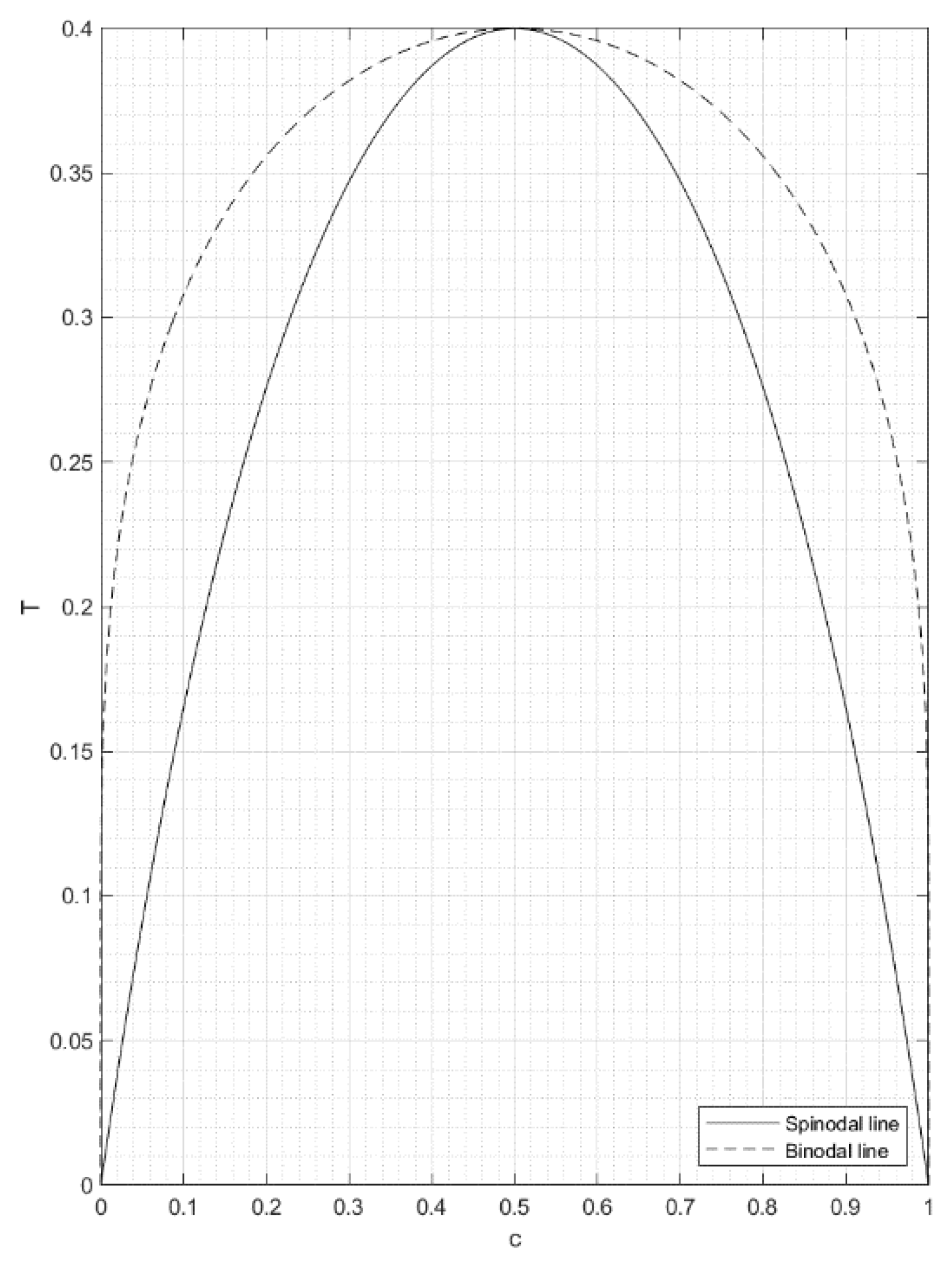
The dependent variable is c^*, and the independent variables are (x^*, y^*, t^*). Equations (8)–(11) are solved numerically for c^*(x^*, y^*, t^*) using the Galerkin finite element method with Hermitian bicubic basis functions to discretize space [31]. A set of non-linear ordinary time-dependent differential equations are obtained after spatial discretization, which are solved simultaneously using the Newton–Raphson iteration method. The mesh size used was 256 × 256, and all simulations were performed on personal computers with Intel Core i7-8700 central processing unit (CPU), 16 GB, and 2666 MHz RAM using MATLAB R2018a [32] with the SuiteSparse built-in package. Convergence is assumed when the length of the vector of the difference of two successive computed solution vector is less than 10⁻⁶. To take advantage of all 6 cores CPU of personal computer, a parallel computation algorithm is implemented. To make the code as efficient as possible, repetitive computations are stored to RAM in an amount that does not compromise the computational speed. The Fourier transform, carried out using the fft function built into MATLAB R2018a [32], is used to compute the structure factor in wavenumber k₁-k₂ space, which simulates the time evolution of light scattering patterns during phase separation. The fft function that is available in MATLAB R2018a [32], and it was added to the program to determine the structure factor of the phase separating morphology. This step with the fft is determined at each time step along with the phase separation morphology. A bright ring with radius that decreases with time is the hallmark observation of phase separation by spinodal decomposition in the unstable region. Light-scattering patterns for phase separated structures formed by spinodal decomposition are depicted by a bright ring in a black background, while a diffuse light-scattering pattern is ubiquitous for droplet nucleation and growth. The parameters are the dimensionless diffusion coefficient D, dimensionless initial average concentration c₀^*, and dimensionless temperature T^*. The binary phase diagram used is shown in Figure 1. Although a comprehensive parametric study was performed on these parameters, the restricted number of simulations presented here best reflect the objectives of this paper.

3. Results and Discussion

3.1. Anisotropic Quenching

Anisotropic quenching is a useful and practical tool to fabricate functional materials. An anisotropic quench occurs when the quenching parameters vary across the domain. The result is normally a non-uniform morphology. For the present model, the deeper the quench is, or the lower it is from spinodal line, the higher is the characteristic frequency. Thus, if the temperature is varied linearly across the domain, one expects smaller droplets or interconnected structures on the deeper quench side.

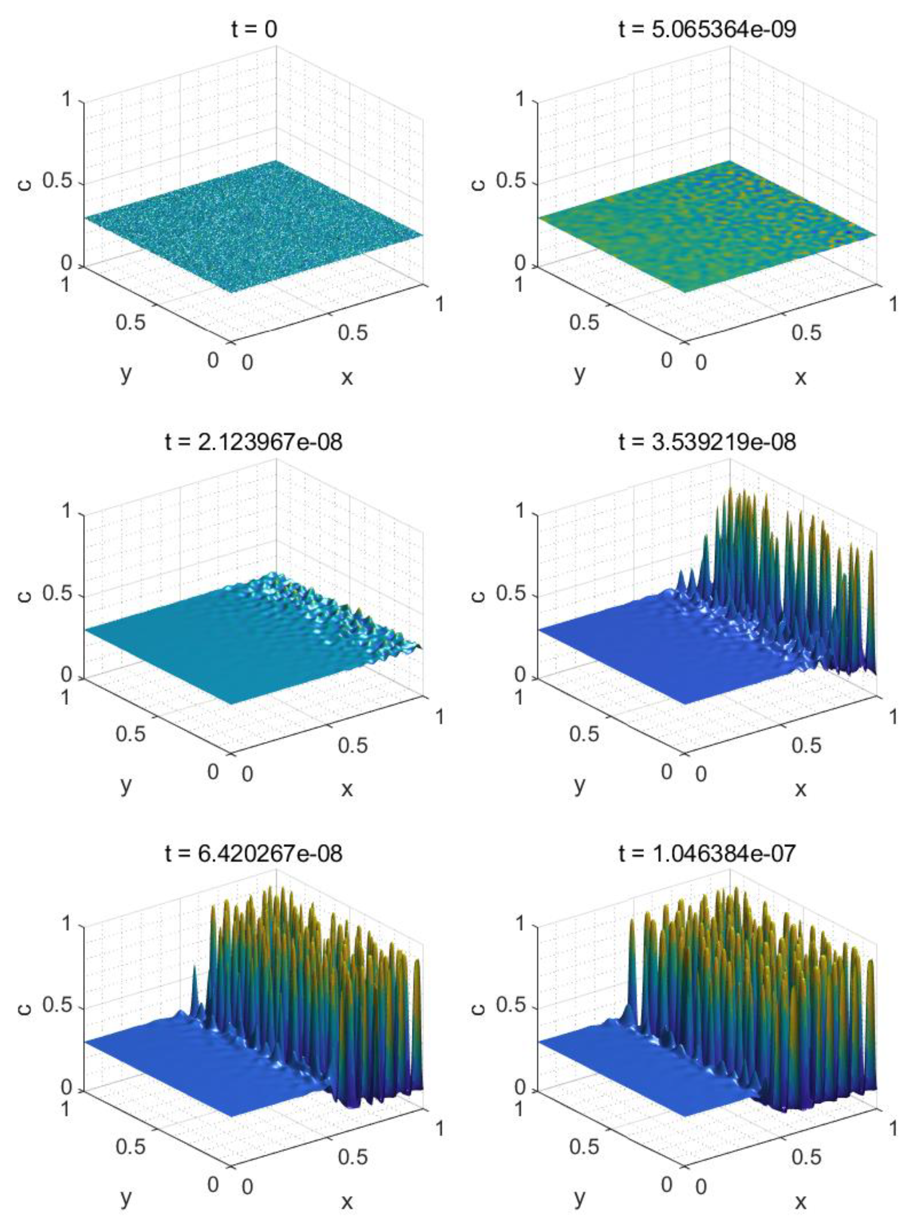
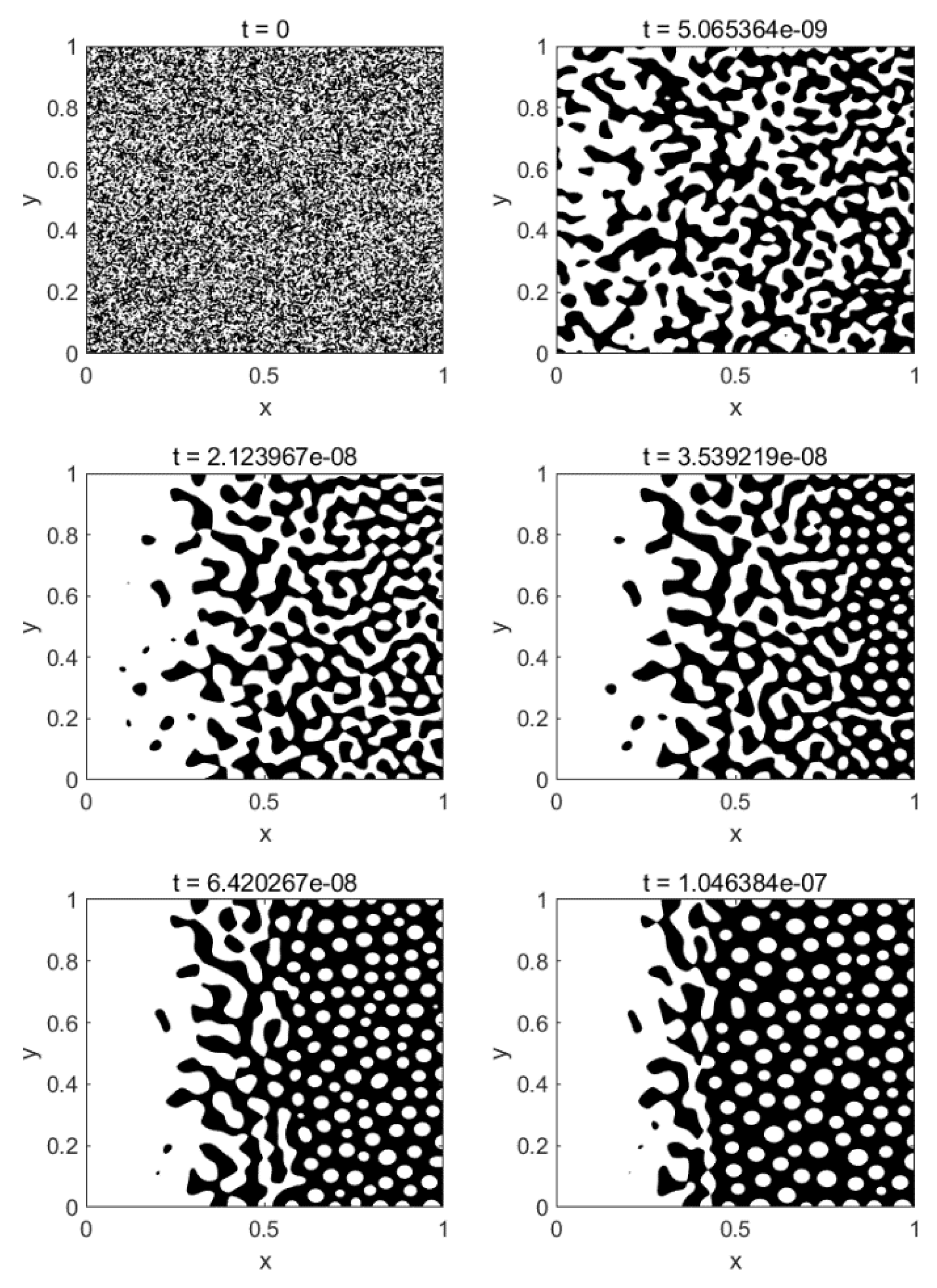
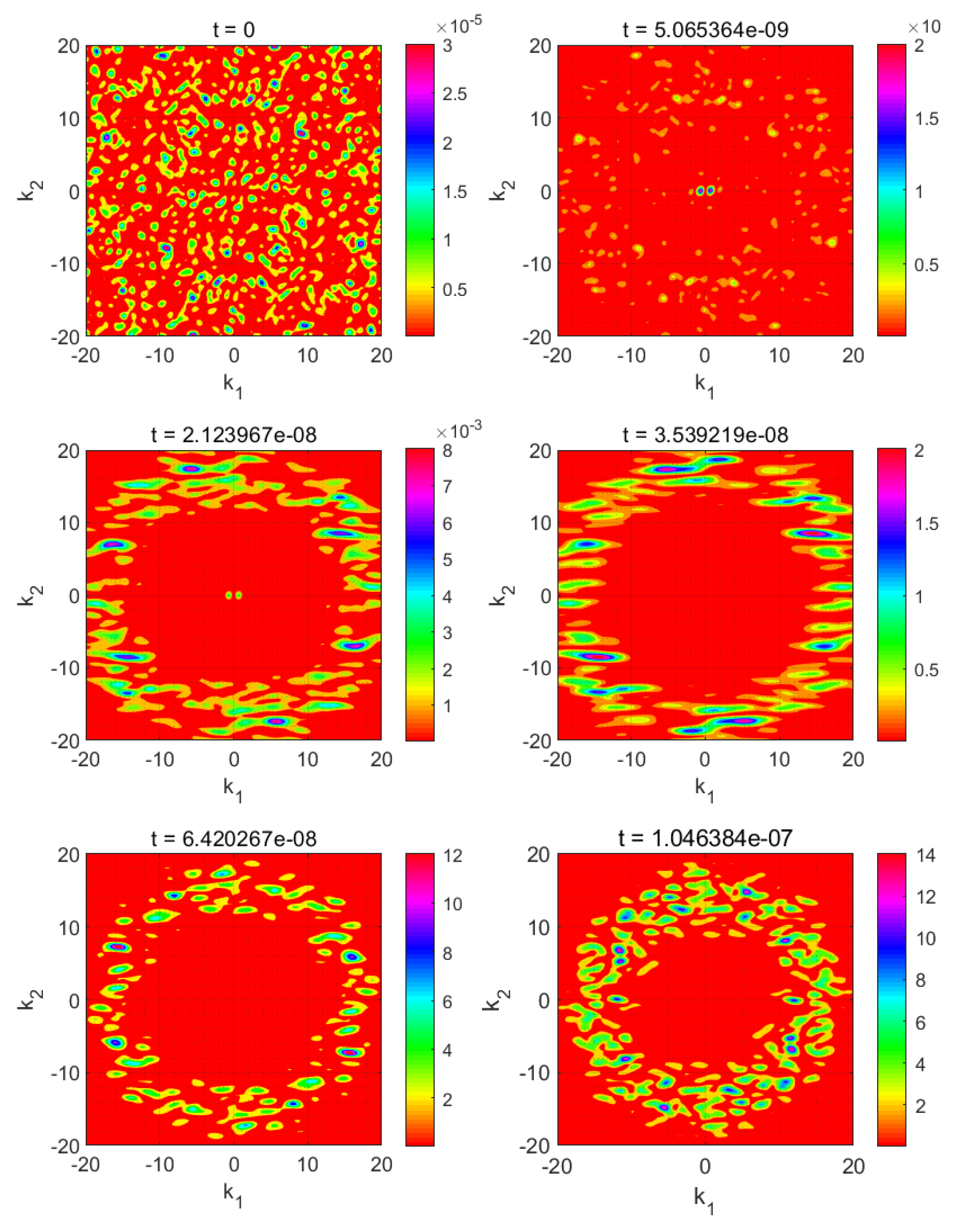
Figure 2 shows the time evolution of the dimensionless concentration profiles c^*(x^*,y^*), while Figure 3 shows the corresponding patterns formed for a binary solution with c₀^* = 0.3, D = 10⁵ and linear temperature variation T₁^* = 0.34 (inside metastable region) at x^* = 0 and T₂^* = 0.30 (inside the unstable region) at x^* = 1. The black regions represent concentrations less than c₀^*, and the white regions represent concentrations greater than c₀^*. These figures show that the concentration fluctuations remain until t^* = 5.065364 × 10⁻⁹. By t^* ≥ 2.123967 × 10⁻⁸, the fluctuations at x^* > 0.5 (unstable region) begin to reorganize into droplets as a result of phase separation by spinodal decomposition, while those at x^* < 0.5 (metastable region) vanish. The fluctuations vanish in the metastable region because their magnitude is not sufficient to overcome the energy activation barrier require for nucleation. Figure 4 shows simulated light-scattering patterns obtained from the structure factor calculations for this case. A ring forms, develops and decreases in diameter, as expected for phase separation by spinodal decomposition in the unstable region.

3.2. Double Quenching

Only small concentration fluctuations at the beginning of the simulation at t^* = 0 are included as noise in the present model. It has been assumed that this mimics the initial state of binary solutions well [19,20,21,22,23]. For phase separation to occur in the metastable state, the solution must overcome a thermodynamic barrier. The solution must have achieved a configuration that is different from a perfectly uniform solution. It is difficult with the present model and specified parameters to initiate phase separation with single quench with only small noise initially, as observed above in Section 3.1. Double quenching occurs when a binary solution is first allowed to phase separate by spinodal decomposition after a quench into the unstable region for some time before it is quenched once more to a lower or higher temperature to continue phase separation either in the unstable or metastable region. A phase-separated morphology will develop in the first quench, thus providing the concentration gradients/fluctuations require for droplet nucleation in the metastable region. Two cases (narrow and wide metastable regions) will be discussed below depending on the gap size between the binodal and spinodal lines.

3.2.1. Narrow Metastable Region

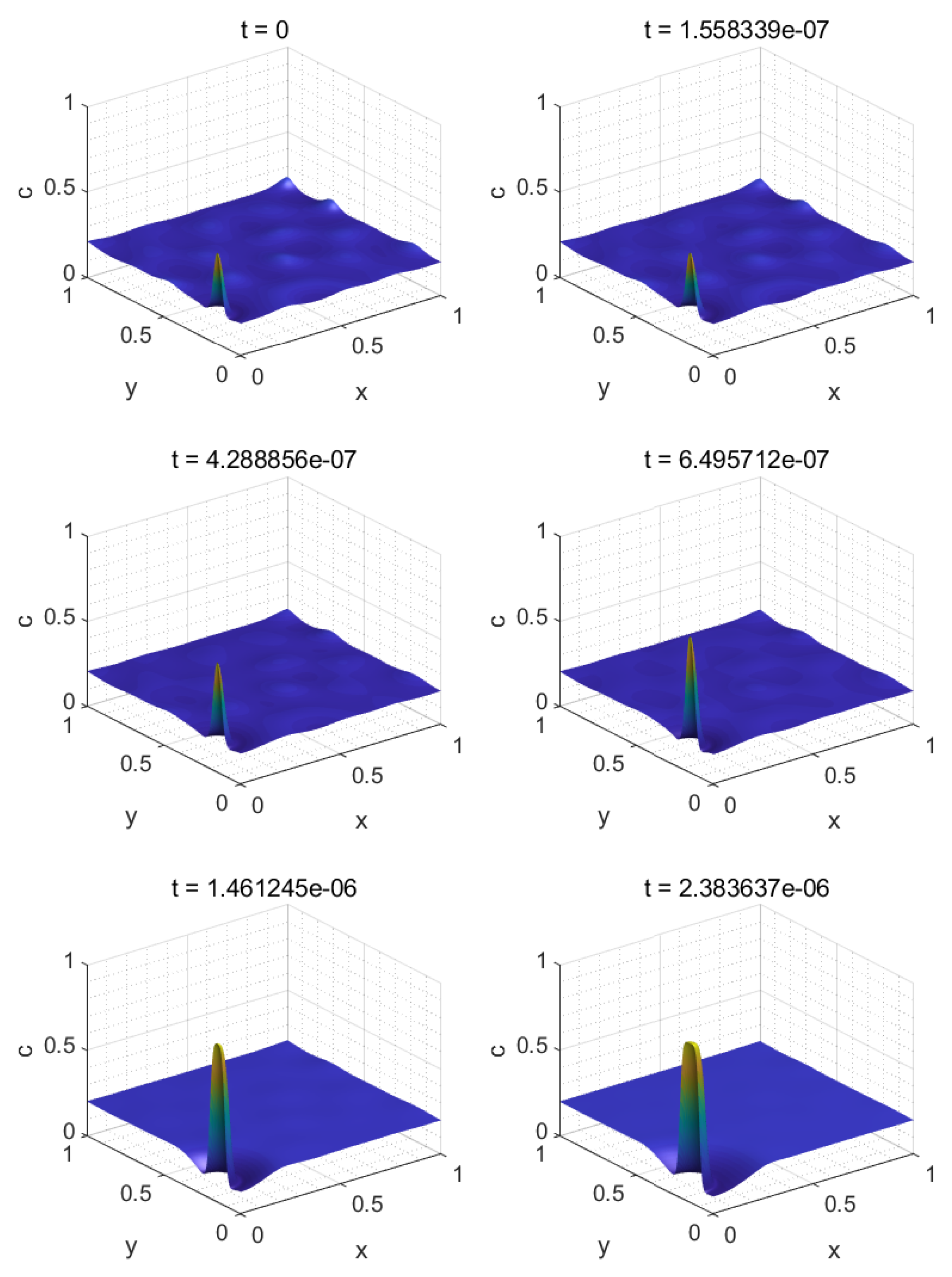
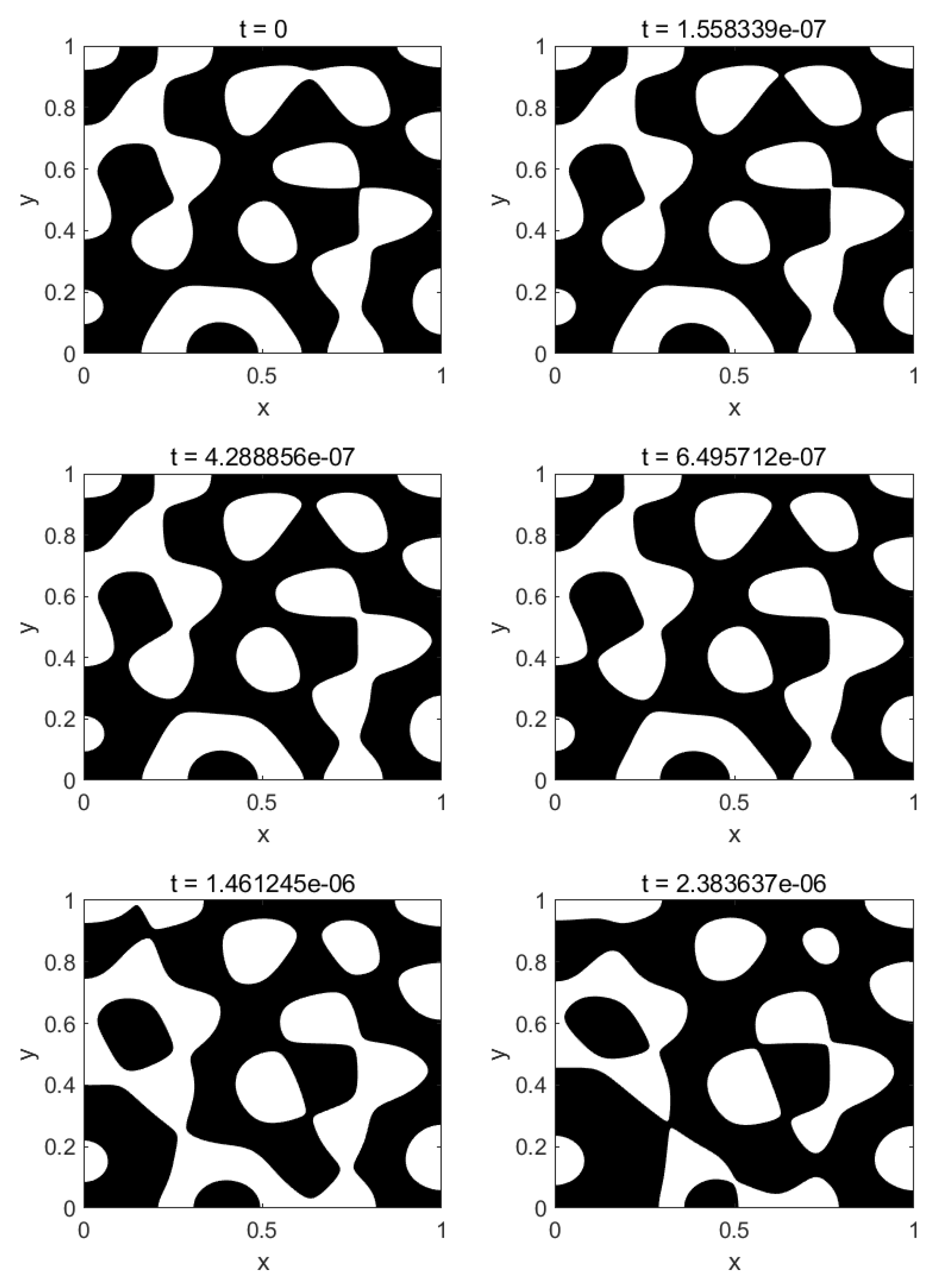
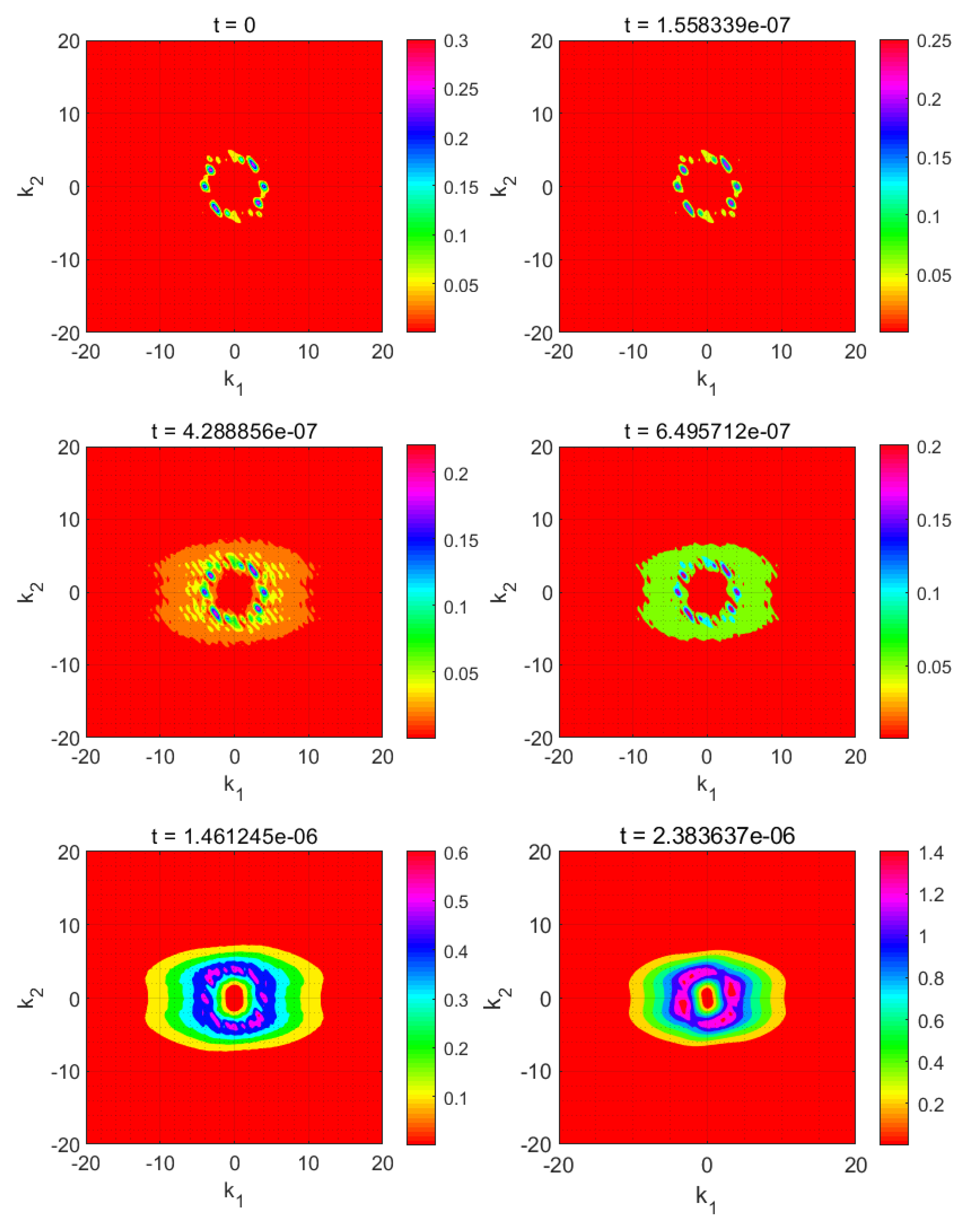
A binary solution with D = 10⁵ and c₀^* = 0.2 is first quenched from the uniform state to T^* = 0.26. It is allowed to phase separate by spinodal decomposition in the unstable region until it reaches t^* = 3.264183 × 10⁻⁵ before the temperature is raised instantaneously to T^* = 0.29 within the narrow metastable region. At this time before the second temperature jump, the binary solution is still in the early stages of phase separation where the fluctuations have not evolved into large concentration variations. The dimensionless concentration profile c^*(x^*,y^*), and the corresponding pattern formed for this binary solution at this dimensionless time are shown as t^* = 0 in Figure 5 and Figure 6, respectively, for the case of the second temperature jump. These two figures show only one major droplet and two minor droplet are formed in the sample before the temperature is raised to T^* = 0.29 (i.e., at t^* = 0) in the narrow metastable region; this droplet provides sufficient concentration fluctuation to overcome the energy barrier for nucleation thus allowing it to continue to grow after the temperature is raised to T^* = 0.29. There are conditions that allow for a major droplet to form faster than minor droplets, as is this case. If the phase separation was allowed to proceed longer, then the major droplet would reach the equilibrium values first while more minor droplets would form and eventually become major ones as well. In the rest of the sample, however, there is no sufficient concentration fluctuation to activate nucleation. Figure 7 shows the simulated light scattering patterns obtained from the structure factor calculations for this case. The ring formed from spinodal decomposition becomes diffuse and decreases in diameter, as expected for transition from phase separation by spinodal decomposition to phase separation by nucleation in the metastable region. The C–H theory is able to predict nucleation and growth close to the spinodal line within the metastable region using a double quench mechanism.

3.2.2. Wide Metastable Region

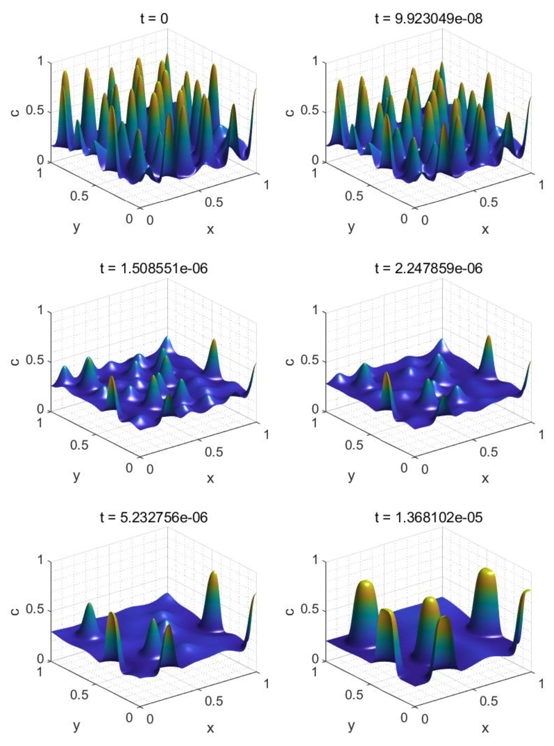
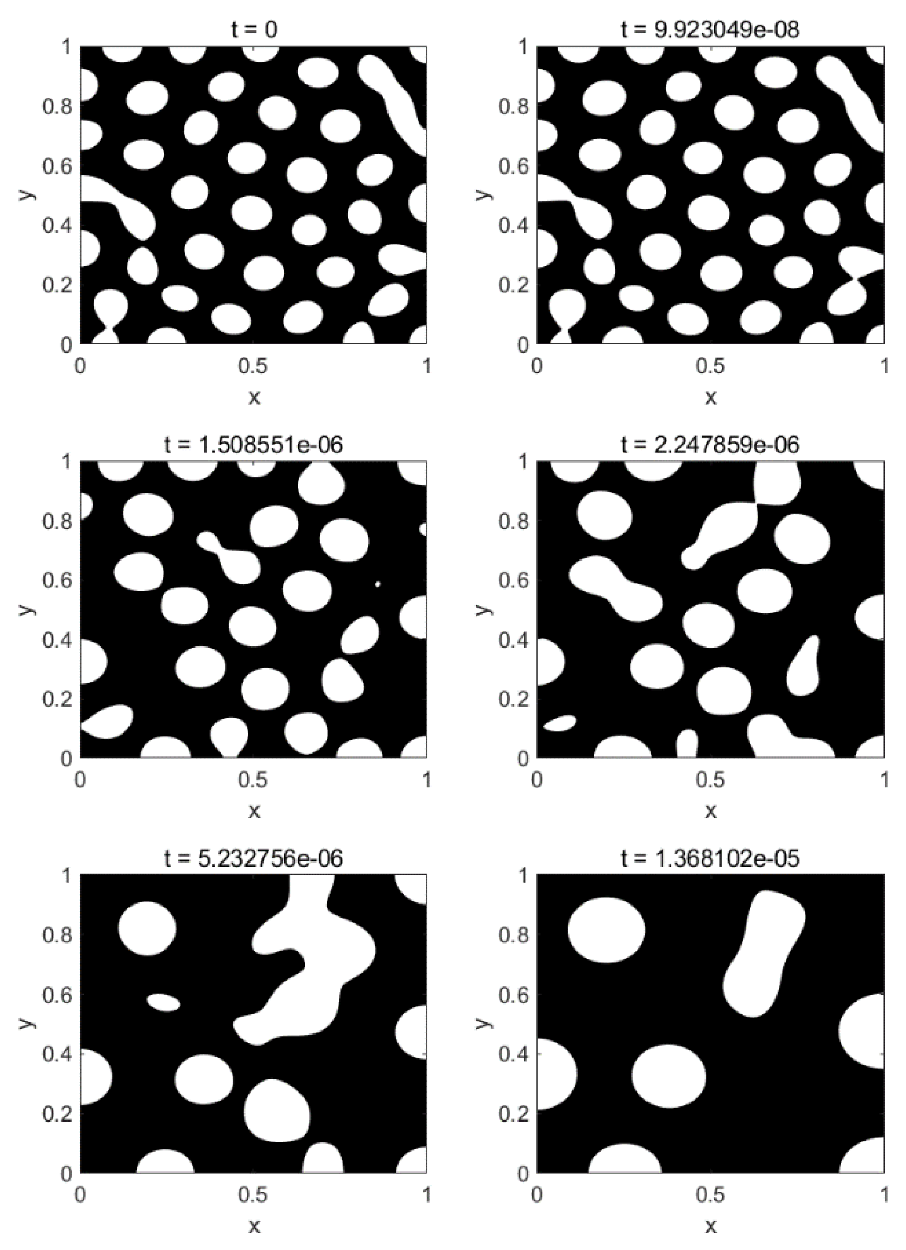
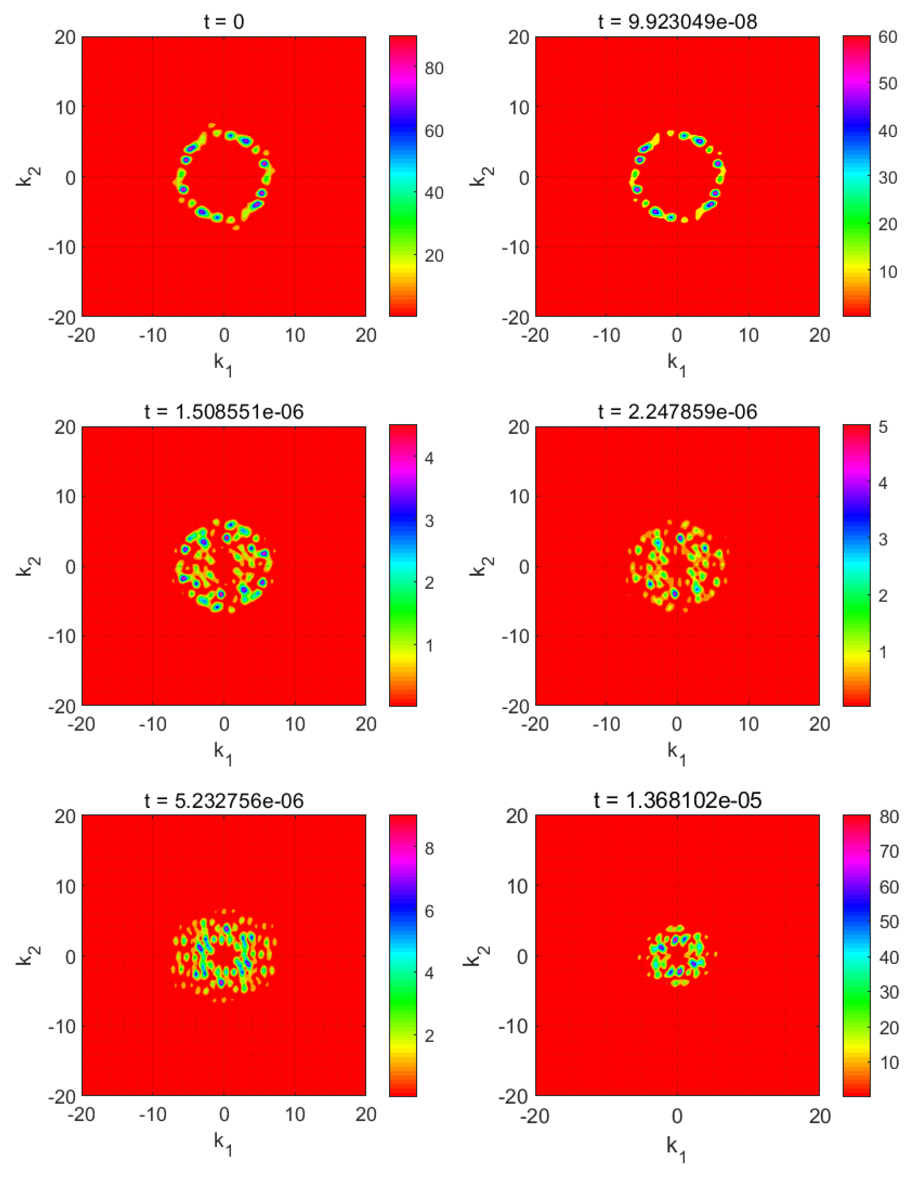
A binary solution with D = 10⁵ and c₀^* = 0.3 is first quenched from the uniform state to T^* = 0.3. It is allowed to phase separate by spinodal decomposition in the unstable region till it reaches t^* = 5.318622 × 10⁻⁶ before it is raised instantaneously to T^* = 0.35, which is within the metastable region but close to the spinodal line. At this time, before the second jump, the binary solution is in the intermediate stage of phase separation where the fluctuations have evolved into large enough concentration variations. The dimensionless concentration profile c^*(x^*, y^*), and the corresponding pattern formed for this binary solution at this dimensionless time are shown as t^* = 0 in Figure 8 and Figure 9, respectively, for the case of the second temperature jump. These two figures show that the concentration fluctuations developed by spinodal decomposition in the unstable region provide sufficient fluctuations to overcome the energy barrier for nucleation in the metastable region after the temperature is raised to T^* = 0.35. Figure 10 shows the simulated light scattering patterns obtained from the structure factor calculations for this case. The ring formed by spinodal decomposition in the first quench is shown at t^* = 0. The ring becomes diffuse and decreases in diameter to a characteristic length predicted by the C–H theory. The C–H theory is able to predict nucleation and growth close to the spinodal line within the metastable region using the double quench mechanism to overcome the thermodynamic barrier.

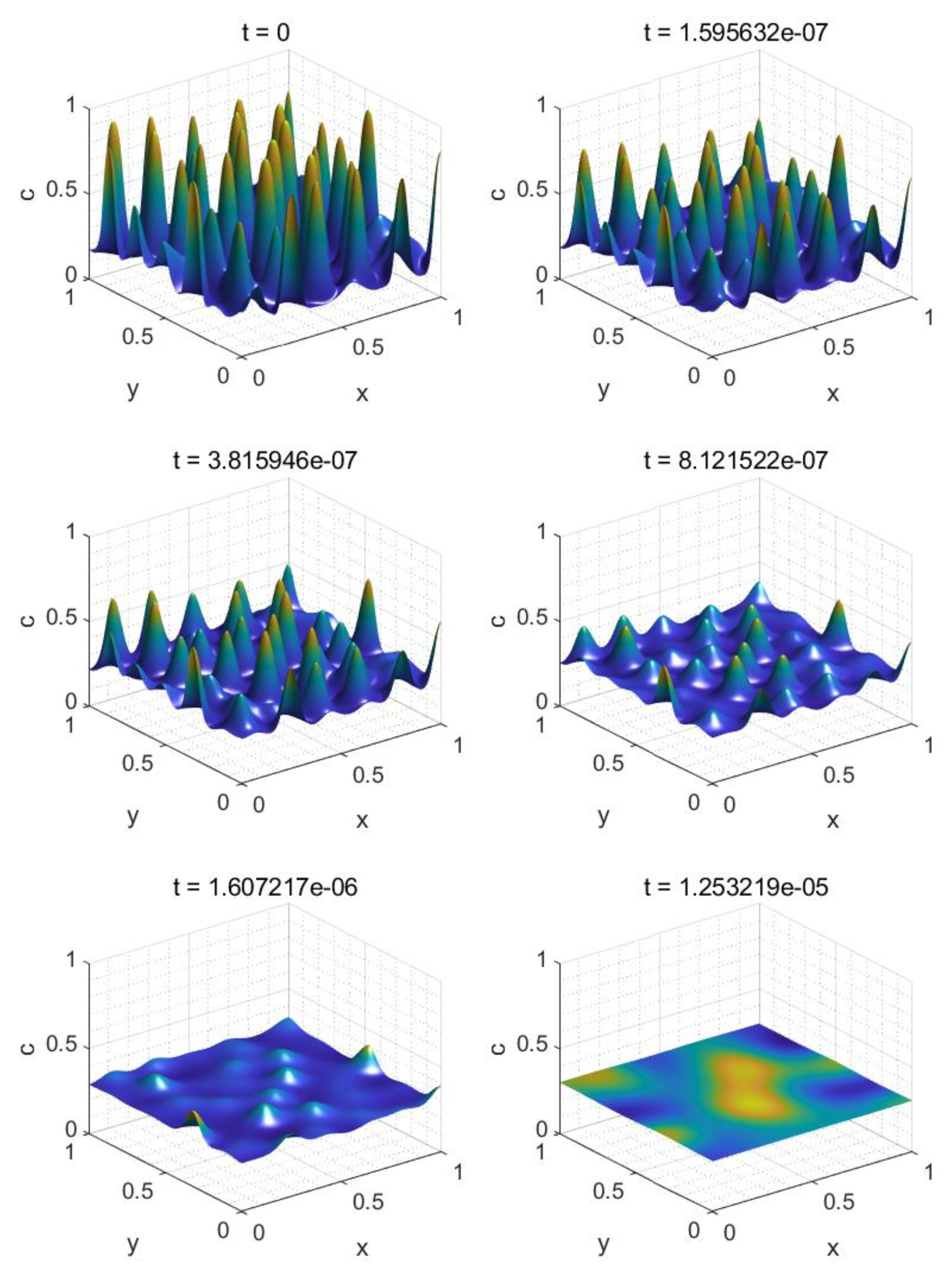
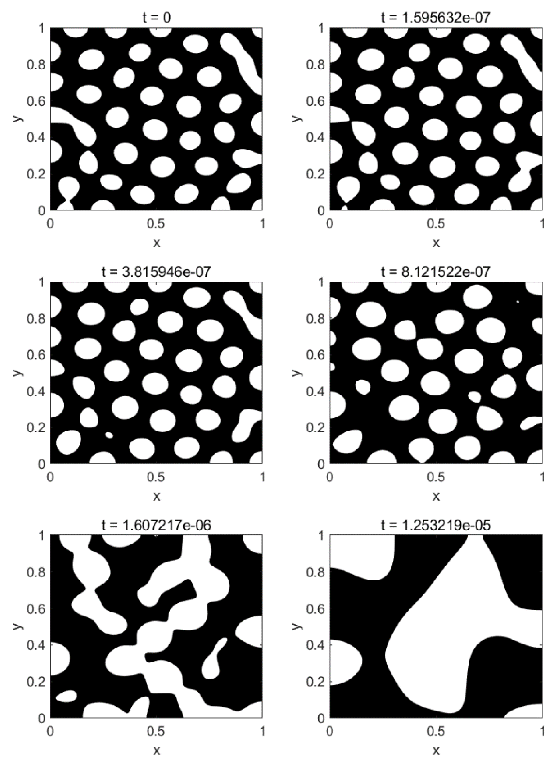
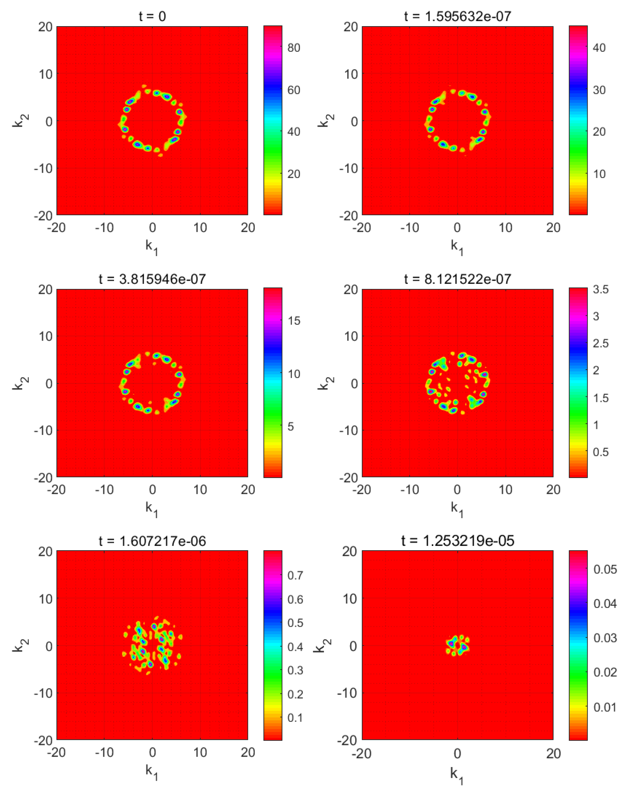
A higher temperature rise into the metastable region (i.e., further away from the binodal line) was also investigated. Using the same binary solution as described above for a quench to T^* = 0.3, the temperature was raised instantaneously to T^* = 0.36 this time instead of T^* = 0.35. Figure 11 and Figure 12 show the time evolution of the dimensionless concentration profiles c^*(x^*, y^*), and the corresponding patterns formed for a binary solution for the case where the temperature is raised quickly to T^* = 0.36. All of the droplets disappear eventually by time t^* = 1.253219 × 10⁻⁵. Figure 13 shows the simulated light-scattering patterns obtained from the structure factor calculations for this simulation. It can be seen that, as the time proceeds, the characteristic ring developed by spinodal decomposition in the first quench vanishes. Therefore, since all the droplets vanish, and there is sufficient concentration gradient initially to overcome the energy barrier for nucleation, the C–H theory is not able to predict the phase separation by nucleation and growth as we move away from the binodal line in the metastable region.

4. Conclusions

The Cahn–Hilliard theory, incorporating Flory–Huggins free energy, was used to mathematically model and numerically simulate the phase separation phenomena in the unstable and metastable regions of a binary low molecular weight solution. No noise term was included in the model, as is normally used for nucleation in the metastable region. Double-quenching was used instead to create concentration gradients for the fluctuations required for nucleation in the metastable region. It was found that the C–H theory is able to simulate nucleation in the metastable region in an area close to the spinodal line. The C–H theory fails to simulate nucleation outside of this area in the metastable region. These numerical results provide insights for experimental studies on producing droplets in the metastable region in addition to the current method of quenching directly into the metastable region to obtain nucleation sites.

References

- Doane, J.W. Polymer dispersed liquid crystal displays. In Liquid Crystals: Applications and Uses; Bahadur, B., Ed.; World Scientific: Singapore, 1990; Volume 1. [Google Scholar]
- Higgins, D.A. Probing the mesoscopic chemical and physical properties of polymer-dispersed liquid crystals. Adv. Mater. 2000, 12, 251–264. [Google Scholar] [CrossRef]
- Barton, B.F.; McHugh, A.J. Modeling the dynamics of membrane structure formation in quenched polymer solutions. J. Membr. Sci. 2000, 166, 119–125. [Google Scholar] [CrossRef]
- Matsuyama, H.; Yuasa, M.; Kitamura, Y.; Teramoto, M.; Lloyd, D.R. Structure control of anisotropic and asymmetric polypropylene membrane prepared by thermally induced phase separation. J. Membr. Sci. 2000, 179, 91–100. [Google Scholar] [CrossRef]
- Dalmoro, A.; Barba, A.A.; Lamberti, G.; Grassi, M.; d’Amore, M. Pharmaceutical applications of biocompatible polymer blends containing sodium alginate. Adv. Polym. Technol. 2012, 31, 219–230. [Google Scholar] [CrossRef]
- Evans, D.F.; Wennerstrom, H. The Colloidal Domain: Where Physics, Chemistry, Biology and Technology Meet, 2nd ed.; Wiley-VCH: New York, NY, USA, 1999. [Google Scholar]
- Norde, W. Colloids and Interfaces in Life Sciences; Marcel Dekker: New York, NY, USA, 2003. [Google Scholar]
- Yaseen, M.; Salacinski, H.J.; Seifalian, A.M.; Lu, J.R. Dynamic protein adsorption at the polyurethane copolymer/water interface. Biomed. Mater. 2008, 3, 034123. [Google Scholar] [CrossRef] [PubMed]
- Mishra, K.; Hashmi, S.A.; Rai, D.K. Nanocomposite blend gel polymer electrolyte for proton battery application. J. Solid State Electrochem. 2013, 17, 785–793. [Google Scholar] [CrossRef]
- Zeng, J.H.; Wang, Y.F.; Gou, S.Q.; Zhang, L.P.; Chen, Y.; Jiang, J.X.; Shi, F. Sulfur in hyper-cross-linked porous polymer as cathode in lithium-sulfur batteries with enhanced electrochemical properties. ACS Appl. Mater. Interfaces 2017, 9, 34783. [Google Scholar] [CrossRef]
- Nyholm, L.; Nystrom, G.; Mihranyan, A.; Stromme, M. Toward flexible polymer and paper-based storage devices. Adv. Mater. 2011, 23, 3751–3769. [Google Scholar] [CrossRef]
- Yamaguchi, T.; Miyata, F.; Nakao, S. Polymer electrolyte membranes with a pore-filling structure for a direct methanol fuel cell. Adv. Mater. 2003, 15, 1198–1201. [Google Scholar] [CrossRef]
- Kimmins, S.D.; Cameron, N.R. Functional porous polymers by emulsion templating: Recentadvances. Adv. Funct. Mater. 2011, 21, 211–225. [Google Scholar] [CrossRef]
- Van Driessche, A.E.S.; Van Gerven, N.; Bomans, P.H.H.; Joosten, R.R.M.; Friedrich, D.G.-C.; Sommerdijk, N.A.J.M.; Sleutel, M. Molecular nucleation mechanisms and control strategies for crystal polymorph selection. Nature 2018, 556, 89–94. [Google Scholar] [CrossRef] [PubMed] [Green Version]
- Sleutel, M.; Van Driessche, A.E.S. Nucleation of protein crystals—A nanoscopic perspective. Nanoscale 2018, 26, 12256–12267. [Google Scholar] [CrossRef] [PubMed]
- Cahn, J.W. Phase separation by spinodal decomposition in isotropic systems. J. Chem. Phys. 1965, 42, 93–99. [Google Scholar] [CrossRef]
- Caneba, G.T.; Soong, D.S. Polymer membrane formation through the thermal-inversion process. 2. Mathematical modeling of membrane structure formation. Macromolecules 1985, 18, 2545–2555. [Google Scholar] [CrossRef]
- Chan, P.K.; Rey, A.D. Computational analysis of spinodal decomposition dynamics in polymer solutions. Macromol. Theory Simul. 1995, 4, 873–899. [Google Scholar] [CrossRef]
- Tran, T.L.; Chan, P.K.; Rousseau, D. Morphology control in symmetric polymer blends using spinodal decomposition. Chem. Eng. Sci. 2005, 60, 7153–7159. [Google Scholar] [CrossRef]
- Clarke, N. Target morphologies via a two-step dissolution-quench process in polymer blends. Phys. Rev. Lett. 2002, 89, 215506. [Google Scholar] [CrossRef]
- Lee, K.-W.; Chan, P.K.; Feng, X. Morphology development and characterization of the phase-separated structure resulting from the thermal-induced phase separation phenomenon in polymer solutions under a temperature gradient. Chem. Eng. Sci. 2004, 59, 1491–1504. [Google Scholar] [CrossRef]
- Hong, S.; Chan, P.K. Simultaneous use of temperature and concentration gradients to control polymer solution morphology development during thermal-induced phase separation. Model. Simul. Mater. Sci. Eng. 2010, 18, 025013. [Google Scholar] [CrossRef]
- Tabatabaieyazdi, M.; Chan, P.K.; Wu, J. A computational study of short-range surface-directed phase separation in polymer blends under a linear temperature gradient. Chem. Eng. Sci. 2015, 137, 884–895. [Google Scholar] [CrossRef]
- Henderson, I.C.; Clarke, N. Two-phase separation in polymer blends. Macromolecules 2004, 37, 1952–1959. [Google Scholar] [CrossRef]
- Tran, T.L.; Chan, P.K.; Rousseau, D. Morphology control in symmetric polymer blends using two-step phase separation. Comput. Mater. Sci. 2006, 37, 328–335. [Google Scholar] [CrossRef]
- Kwak, K.D.; Okada, M.; Chiba, T.; Nose, T. Growth rate of microdomains during phase separation by a two-step temperature jump. Macromolecules 1993, 26, 4047–4049. [Google Scholar] [CrossRef]
- Cahn, J.W.; Hilliard, J.E. Free energy of a nonuniform system. III. Nucleation in a two-component incompressible fluid. J. Chem. Phys. 1959, 31, 688–699. [Google Scholar] [CrossRef]
- Bates, P.W.; Fife, P.C. The dynamics of nucleation for the Cahn-Hilliard equation. SIAM J. Appl. Math. 1993, 53, 990–1008. [Google Scholar] [CrossRef]
- Kyu, T.; Lee, J.-H. Nucleation initiated spinodal decomposition in a polymerizing system. Phys. Rev. Lett. 1996, 76, 3746–3749. [Google Scholar] [CrossRef]
- Flory, P.J. Principles of Polymer Chemistry; Cornell University Press: Ithaca, NY, USA, 1953. [Google Scholar]
- Lapidus, L.; Pinder, G.F. Numerical Solution of Partial Differential Equations in Science and Engineering; John Wiley: New York, NY, USA, 1999. [Google Scholar]
- MATLAB for Artificial Intelligence. Available online: http://www.mathworks.com.
Figure 1.
Binary phase diagram for N1 = N2 = 1 and Ψ = 1.
Figure 2.
Dimensionless concentration spatial profiles c*(x*, y*) formed during the phase separation phenomena for the case where D = 105, co* = 0.3 and T1* = 0.34 at x* = 0 and T2* = 0.30 at x* = 1. The asterisks were left out of the variables x, y, c, and t in the figure.
Figure 3.
Patterns formed during the phase separation phenomena for the case where D = 105, co* = 0.3 and T1* = 0.34 at x* = 0 and T2* = 0.30 at x* = 1. The asterisks were left out of the variables x, y, and t in the figure.
Figure 4.
Simulated light scattering patterns obtained for the calculated structure factors for the case where D = 105, co* = 0.3 and T1* = 0.34 at x* = 0 and T2* = 0.30 at x* = 1. The asterisks were left out of the variables k1, k2, and t in the figure.
Figure 5.
Dimensionless concentration spatial profiles c*(x*, y*) formed during the phase separation phenomena for the case where D = 105, co* = 0.2 and T* = 0.29. The asterisks were left out of the variables x, y, c, and t in the figure.
Figure 6.
Patterns formed during the phase separation phenomena for the case where D = 105, co* = 0.2 and T* = 0.29 at x* = 0 and T2* = 0.30 at x* = 1. The asterisks were left out of the variables x, y, and t in the figure.
Figure 7.
Simulated light scattering patterns obtained from the calculated structure factors for the case where D = 105, co* = 0.2 and T* = 0.29. The asterisks were left out of the variables k1, k2, and t in the figure.
Figure 8.
Dimensionless concentration spatial profiles c*(x*, y*) formed during the phase separation phenomena for the case where D = 105, co* = 0.3 and T* = 0.35. The asterisks were left out of the variables x, y, c, and t in the figure.
Figure 9.
Patterns formed during the phase separation phenomena for the case where D = 105, co* = 0.3 and T* = 0.35. The asterisks were left out of the variables x, y, and t in the figure.
Figure 10.
Simulated light scattering patterns obtained from the calculated structure factors for the case where D = 105, co* = 0.3 and T* = 035. The asterisks were left out of the variables k1, k2, and t in the figure.
Figure 11.
Dimensionless concentration spatial profiles c*(x*, y*) formed during the phase separation phenomena for the case where D = 105, co* = 0.3 and T* = 0.36. The asterisks were left out of the variables x, y, c, and t in the figure.
Figure 12.
Patterns formed during the phase separation phenomena for the case where D = 105, co* = 0.3 and T* = 0.36. The asterisks were left out of the variables x, y, and t in the figure.
Figure 13.
Simulated light-scattering patterns obtained from the calculated structure factors for the case where D = 105, co* = 0.3 and T* = 036. The asterisks were left out of the variables k1, k2, and t in the figure.
© 2019 by the authors. Licensee MDPI, Basel, Switzerland. This article is an open access article distributed under the terms and conditions of the Creative Commons Attribution (CC BY) license (http://creativecommons.org/licenses/by/4.0/).
Share and Cite
MDPI and ACS Style
Tran Duc, V.-N.; Chan, P.K. Using the Cahn–Hilliard Theory in Metastable Binary Solutions. ChemEngineering 2019, 3, 75. https://0-doi-org.brum.beds.ac.uk/10.3390/chemengineering3030075
AMA Style
Tran Duc V-N, Chan PK. Using the Cahn–Hilliard Theory in Metastable Binary Solutions. ChemEngineering. 2019; 3(3):75. https://0-doi-org.brum.beds.ac.uk/10.3390/chemengineering3030075
Chicago/Turabian StyleTran Duc, Viet-Nhien, and Philip K. Chan. 2019. "Using the Cahn–Hilliard Theory in Metastable Binary Solutions" ChemEngineering 3, no. 3: 75. https://0-doi-org.brum.beds.ac.uk/10.3390/chemengineering3030075