A Coarse Grained Model for Viscoelastic Solids in Discrete Multiphysics Simulations


1
School of Chemical Engineering, University of Birmingham, Birmingham B15 2TT, UK
2
Industrial Engineering Department, Petra Christian University, Surabaya 60236, Indonesia
*
Author to whom correspondence should be addressed.
ChemEngineering 2020, 4(2), 30; https://0-doi-org.brum.beds.ac.uk/10.3390/chemengineering4020030
Submission received: 10 March 2020
/
Revised: 16 April 2020
/
Accepted: 25 April 2020
/
Published: 1 May 2020
(This article belongs to the Special Issue Discrete Multiphysics: Modelling Complex Systems with Particle Methods)
Abstract
:Viscoelastic bonds intended for Discrete Multiphysics (DMP) models are developed to allow the study of viscoelastic particles with arbitrary shape and mechanical inhomogeneity that are relevant to the pharmaceutical sector and that have not been addressed by the Discrete Element Method (DEM). The model is applied to encapsulate particles with a soft outer shell due, for example, to the partial ingress of moisture. This was validated by the simulation of spherical homogeneous linear elastic and viscoelastic particles. The method is based on forming a particle from an assembly of beads connected by springs or springs and dashpots that allow the sub-surface stress fields to be computed, and hence an accurate description of the gross deformation. It is computationally more expensive than DEM, but could be used to define more effective interaction laws.
1. Introduction
The Discrete Element Method (DEM) has been employed to study a range of pharmaceutical manufacturing processes and products including powder mixing [1], agglomeration with and without a liquid binder [2], and the release of Active Pharmaceutical Ingredients (APIs) from powder inhalation products [3]. Invariably, this has not involved inhomogeneous particles, and those of arbitrary shape have been simulated by gluing primary particles together such that the interior is essentially rigid in order to minimise the computational cost, which is not representative of real particles [4]. An important example of mechanical inhomogeneity is the softening of particles due the presence of moisture during agglomeration or dispersion/dissolution. In such cases, a gradient of moisture content is developed with a corresponding gradient in the mechanical properties. Another example is the encapsulation of APIs for which there is commonly a hard shell and a softer core. For particles formed from an organic polymer such as microcrystalline cellulose, the ingress of moisture will cause them to become viscoelastic.
Mesh-free methods and, in particular, particle methods such as DEM are increasingly popular in the scientific community due to their ability to overcome some drawbacks of the conventional, mesh-based, numerical methods; see [5] for a review. Particle methods can also be coupled together within a Discrete Multiphysics (DMP) framework that, unlike conventional multiphysics techniques, is based on “computational particles” rather than on computational meshes [6,7]. In fact, there is a range of systems for which DMP can address problems that would be very difficult, if not impossible, for traditional multiphysics approaches. Examples are cardiovascular valves [8,9], blood clotting [10], phase transitions [11], capsules’ breakup [12,13], and fuzzy boundaries (e.g., a tablets’ dissolution) [14]. In many of the above examples, the solid phase is often represented by a Lattice Spring Model (LMS) and involves both linear and non-linear springs for modelling elastic materials. In the current study, the method is extended to viscoelastic materials by implementing the Kelvin–Voigt (KV) viscoelastic model that involves springs and also dashpots to represent the viscous friction.
KV bonds have been proposed in the LSM literature, but only to model wave propagation in viscoelastic media (e.g., seismic wave propagation [15]), where the media are treated as homogenous and no external forces are applied to the system. KV bonds have never been implemented to study the strain field of solid objects under the effect of external loads. Achieving this objective would provide particle-based multiphysics techniques (e.g., DMP) with the ability to model viscoelastic materials, which is currently not possible.
The current study addresses the above shortcoming in the literature. For benchmark and validation purposes, the diametric compression of homogeneous spherical particles between parallel platens is described, which may be considered as a special case of indentation. A flat indenter or platen is widely used especially for the diametric compression of single particles [16] and microcapsules [17]. Generally, they are loaded at a constant velocity to a specified displacement and unloaded, or alternatively held in position, to measure the stress relaxation.
A quasistatic model based on Hertz’s contact theory has been employed to describe the interaction between the particles that are packed together to represent unconsolidated porous media [18]. The evolution of the permeability with the deformation was computed by the lattice-Boltzmann approach. Here, the approach is that macroscopic bodies (such as particles) are sub-divided into computational beads. Each bead is connected to the nearest neighbours by linear springs or by KV bonds. It will be shown that for the spherical particle represented by beads connected by linear springs model, under diametric compression simulation, the relationship between force and displacement is nearly identical to the Hertz contact theory.
In the current work, the KV model is compared initially with the theoretical results for a single viscoelastic bond. Then, elastic and viscoelastic spherical particle models including multiple bonds are developed and simulated under diametrical loading. Finally, applications of DMP to spherical particles composed of core and shell regions with different properties are also presented to demonstrate the potential for inhomogeneous systems.
2. Materials and Methods
2.1. Theoretical Background
2.1.1. Hertz Theory for Elastic Normal Contact Force
Hertz proposed a theory to analyse the contact of two elastic isotropic spherical solids by assuming linear elasticity and frictionless boundary conditions [19]. For diametric compression, a spherical body is in contact with two flat surfaces, and the radius of curvature of the flat surfaces is set to infinity. Since the total deformation is evaluated, it is divided by two [20], and therefore, the relationship between the force, , and the relative displacement of the plates, δ, is as follows:
where E, R, and υ are the Young’s modulus, radius, and Poisson’s ratio of the particle, respectively.
2.1.2. Viscoelastic Normal Contact Force
For the diametric compression of a spherical viscoelastic particle, the force may be partitioned between the elastic deformation and the viscoelastic dissipation, thus [21,22]:
where δ and are the displacement and the rate of displacement, respectively. The elastic term is the Hertzian contact force where A is the constant in the Hertz theory. The dissipative part has a dissipative constant B that was derived independently in [21,23,24].
2.1.3. Mass-Spring-Dashpot Models
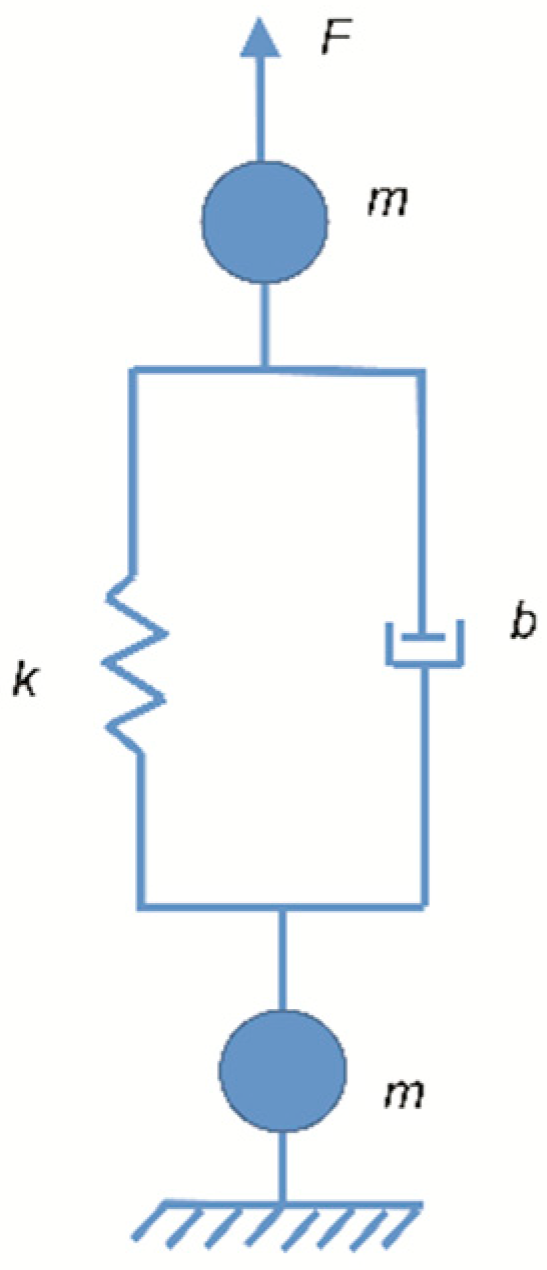
Figure 1 depicts two particles of mass m connected by a KV model, which is defined as a “KV” bond and implemented numerically as described in the next section. When a KV bond is displaced by a distance X from its equilibrium position, the resulting force is given by the following relationship:
where k is the spring constant and b is the dashpot constant. If such a force is applied to the model, the displacement will be a function of time, t, as follows:
2.2. Model and Simulation
In this section, we initially compare the numerical implementation of the spring and dashpot model with the theoretical results for a single viscoelastic bond. Then, we extend the study to a large geometry (spherical) including multiple bonds.
2.2.1. Validation of a Single KV Bond
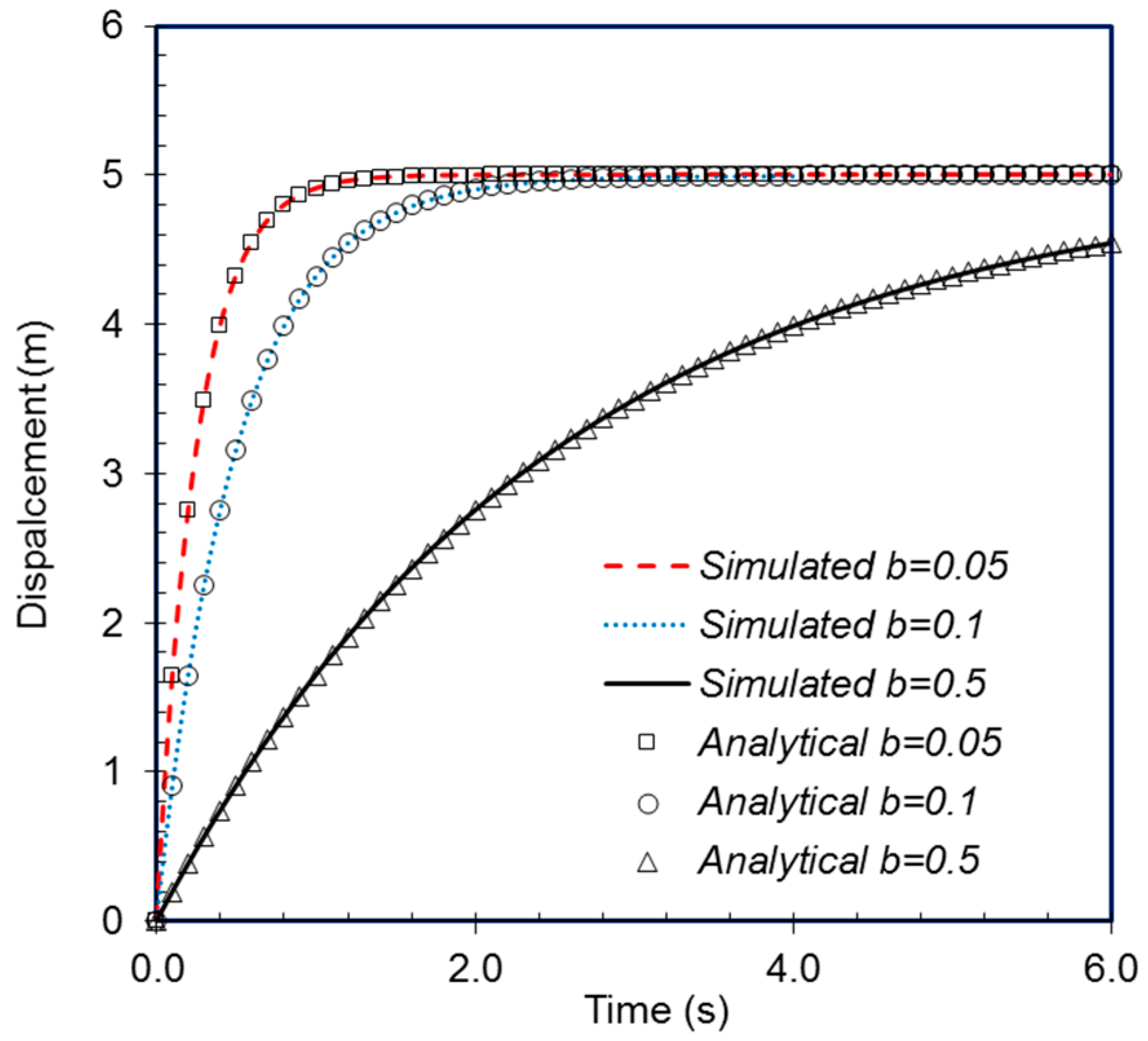
The KV bond was implemented numerically in LAMMPS [25] following the standard Hooke’s law and Newton’s law of fluid flow for the spring and dashpot, respectively, as shown in Equation (3). To validate the numerical implementation of the mass-spring-dashpot model, a simple system was created as shown in Figure 1, and the displacement was calculated from the simulations and compared to the analytical solution of Equation (4). The following parameter values were employed for the simulations: F = 1 N, m = 0.00001 kg, k = 0.2 N/m, and a range of values of b, as shown in Figure 2, where m is the mass of the beads. The simulated displacements are in close agreement with the analytical solution.
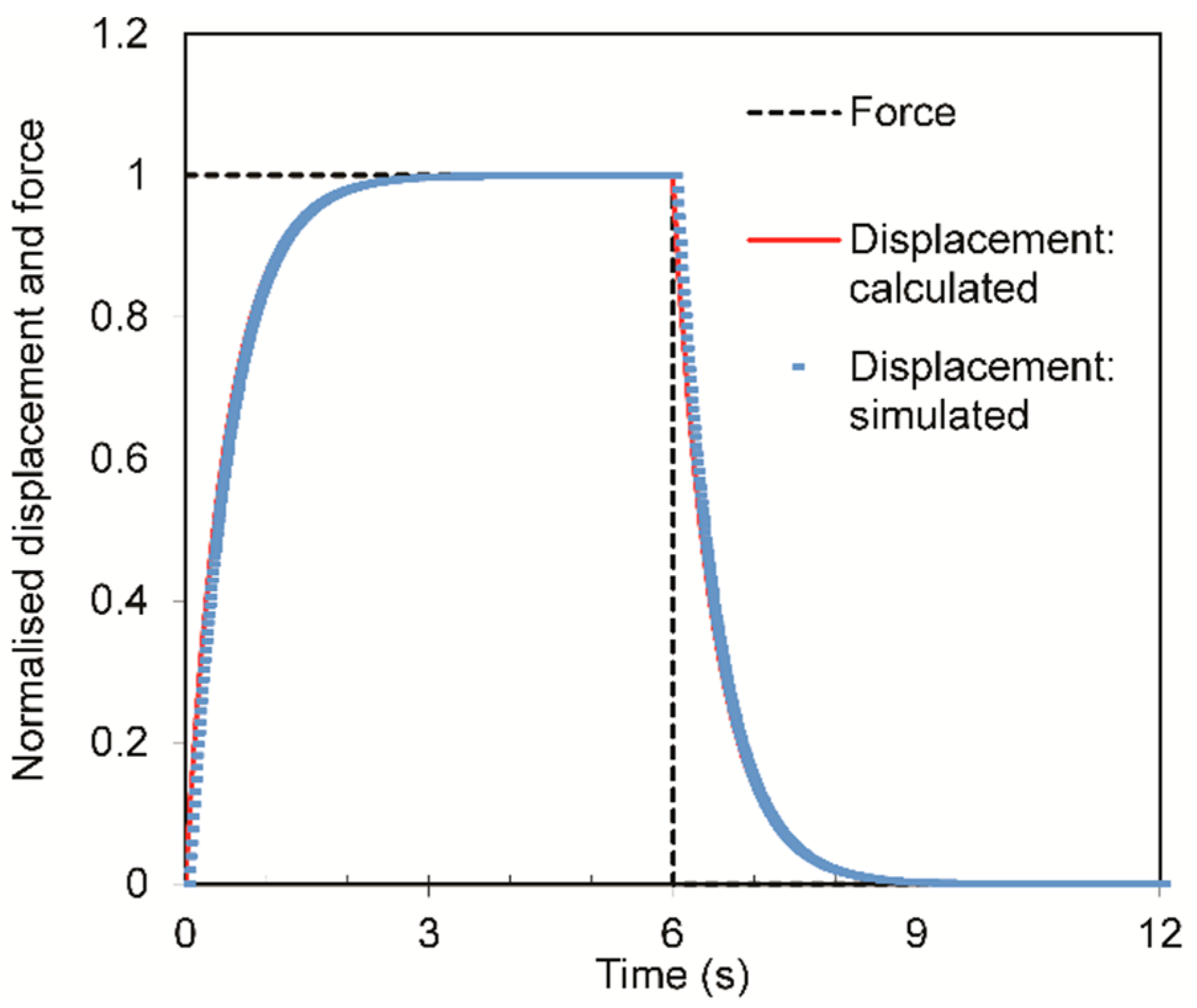
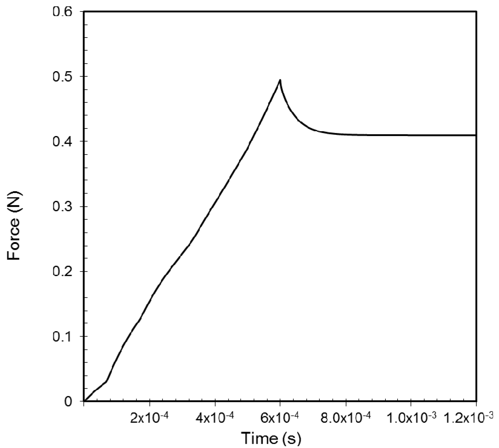
A second validation was performed by comparing the creep and recovery responses of the system in Figure 1 to that calculated using Simulink (Version 9.1, The MathWorks Inc., Natick, MA, USA). As depicted in Figure 3, the simulated displacements were in close agreement with the calculated values from Simulink. After the force was applied, the displacement increased rapidly until it reached a steady state. When the force was removed, the displacement decreased rapidly, and as time increased, it approached asymptotically to zero.
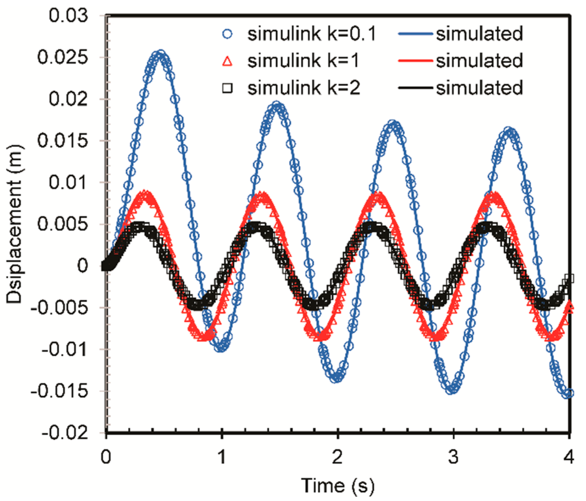
A third validation was performed by comparing the displacement response of the system in Figure 1 to a sinusoidal load (dynamic force), to the value calculated using Simulink (Version 9.1, The MathWorks Inc. Natick, MA, USA), as shown in Figure 4. Furthermore, in this case, the simulated displacements were in close agreement with the calculated values.
2.2.2. Modelling the Diametric Compression of a Spherical Particle
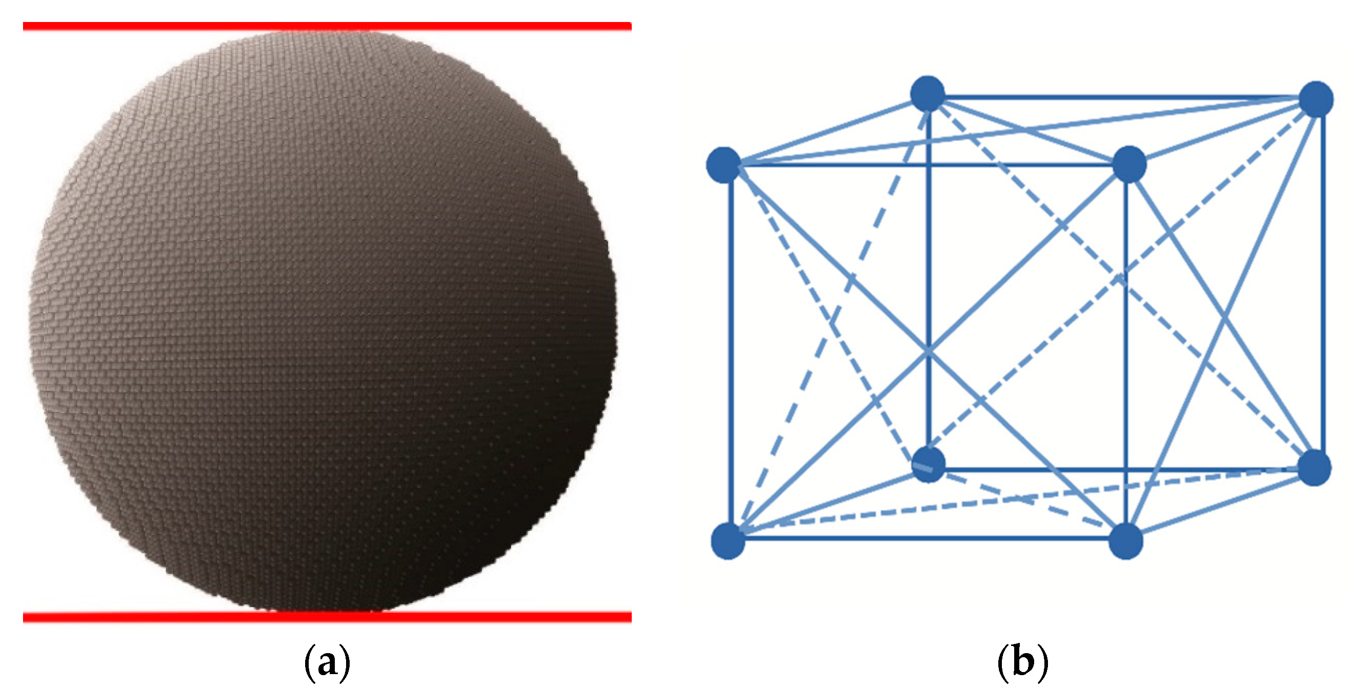
In DMP models, macroscopic bodies are sub-divided into computational particles (beads). Since in this work, we study KV bonds that can be used in DMP (or other particle-based multiphysics methods), we extended the validation to macroscopic spheres that accounted for multiple KV bonds. A sphere could be sub-divided into computational beads in different ways. Here, we employed two approaches: the beads were arranged on (a) a regular cubic lattice and (b) an irregular tetrahedral lattice.
In the first case, the spherical particle (Figure 5a) was constructed from cubic lattice cells (Figure 5b). It contained 137,059 beads with each connected to the nearest neighbours and along face diagonals by linear springs or by KV bonds. This work focuses on viscoelasticity (KV bonds), and the case of purely elastic spheres (linear springs) was computed for comparison. The case of linear springs, in fact, has been already studied, and mass-spring cubic lattice cell models are known to represent (purely) elastic homogenous isotropic materials if the connection between the masses and the stiffness of the springs are selected appropriately [26]. For a cubic lattice cell with nearest neighbour and next nearest-neighbour linear springs, the Poisson’s ratio is predicted by the theory to be 0.25 [26], and Young’s modulus is given by the following relationship [27]:
where l is the length of an edge of the cell. In the “Results and Discussion” (Section 3), our model will be initially validated against these theoretical values for a perfectly elastic sphere by only accounting for linear springs and, later, it will be extended to a viscoelastic sphere by substituting the springs with KV bonds.
E = 2.5 k/l
The tetrahedral cells were created by discretising the sphere with a finite-element mesh generator. In this case, the distance between the beads was not perfectly uniform, and for this reason, we called it a disordered model. Using this approach, less beads were required, but the calculation of the elastic modulus a priori (Equation (5)) was less accurate [26]. A spherical particle based on a disorder model with 5921 beads was created using an open-source 3D finite element grid generator [28]. As in the case of the cubic lattice, the beads were connected to their neighbours either with linear springs or KV bonds to model, respectively, elastic and viscoelastic materials.
Two parallel solid planes were applied to the particle in order to simulate diametric compression. They exerted a force to compress the particle, where the magnitude of the force, F(r), is given by [29]:
where S is the specified force constant, Ri is the position of the plane and rb − Ri is the distance from the bead to the plane. The force is repulsive, and F(r) = 0 for rb > Ri. The force constant was set to be 1010 Nm−2 for all simulations in order to represent rigid compression planes. During the compression loading simulations, one plane compressed the particle with a constant velocity for both the elastic and viscoelastic particle models, while the other was maintained static. For the viscoelastic particle, the displaced plane was held at its final position after the loading to allow for relaxation. The force and particle displacement were recorded during the simulations, and a time step of 10−11 s was used to integrate Newton’s equations of motion.
F(r) = S(rb − Ri)2,
It is well known that the KV model can produce the creep and recovery responses of a two-bead system, as shown in Figure 3, but cannot model stress relaxation behaviour. However, as will be shown in the next section, for the many-bead spherical particle models connected with KV bonds, stress relaxation behaviour could be observed. This is because a many-bead particle model connected with KV bonds is similar to a generalized KV model, i.e., a viscoelastic material model composed of N Kelvin–Voigt units assembled in series. The generalized KV model has been employed, for example to study the viscoelastic properties of micro-cracked materials [30].
3. Result and Discussion
3.1. Perfectly Elastic Spherical Particles
3.1.1. Cubic Lattice Cell Model
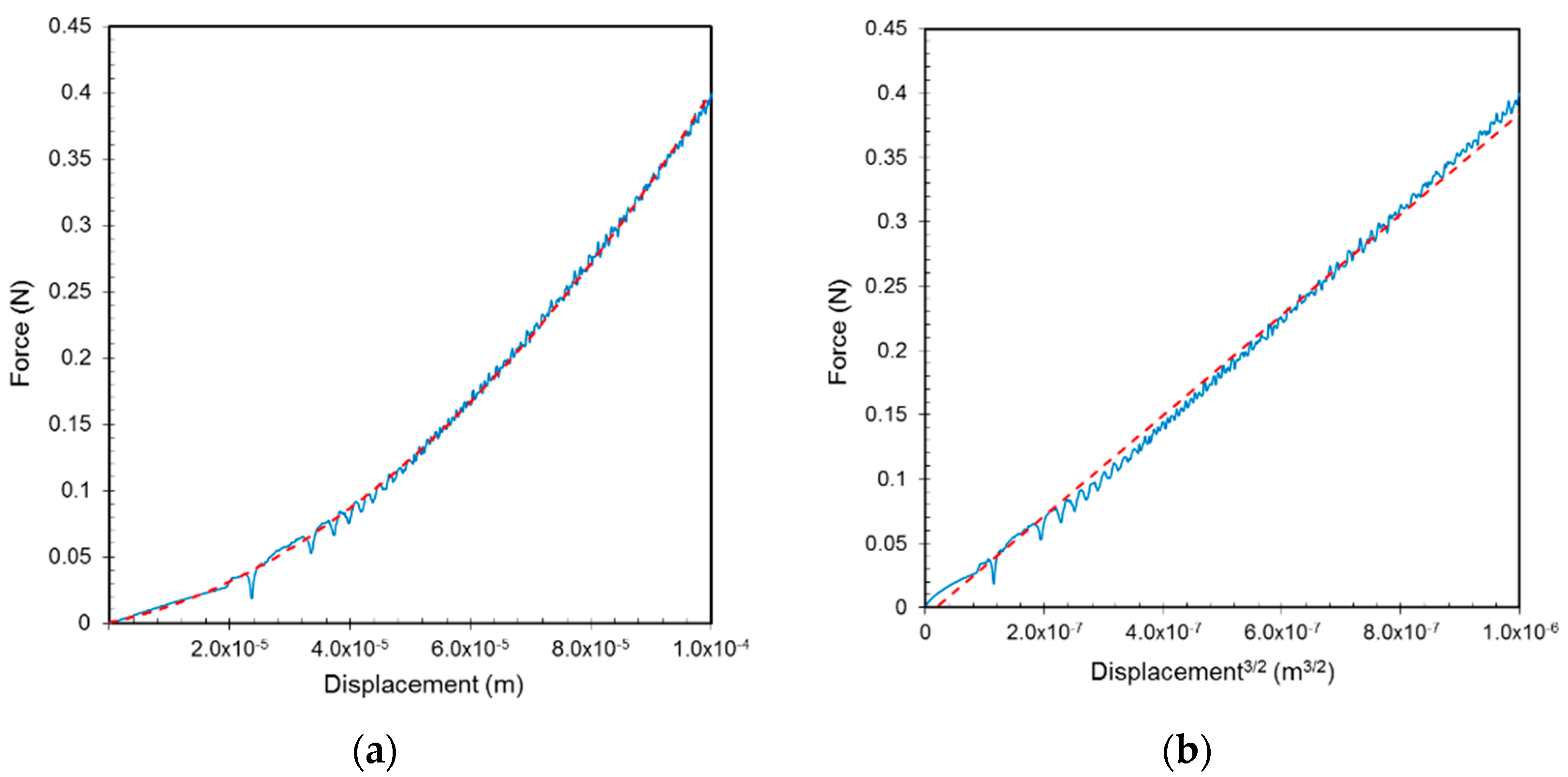
Figure 6a presents the simulated force as a function of displacement for an elastic spherical particle based on the cubic lattice cell with a spring constant of 200 Nm−1. The data were compared against the Hertz theory predictions (Equation (1)) and the comparison depicted in Figure 6b. The force and displacement calculated from the simulations were nearly identical to the Hertz theory. The fluctuating behaviour in Figure 6 was due to slight numerical inaccuracies that artificially perturbed the total energy of the system. Since the particle was perfectly elastic, this energy was never dissipated and manifested itself as a high frequency perturbation. This is a known issue with the LSM, which, in the literature, is usually solved by adding a small artificial dissipative term that damps these high frequencies [31]. In this study, since the focus was on validation, we did not implement any artificial dissipation.
The calculated Young’s modulus for the spherical particle was 39.1 MPa, which was in a close agreement with the Young’s modulus of the elementary cubic lattice cell of 40 MPa calculated using Equation (5). The small discrepancy arose because, due to the cubic cell internal structure, the bead model was not a perfect spherical shape, so that it did not fully comply with the Hertzian contact model.
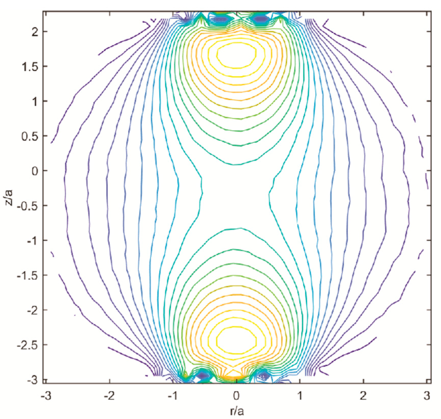
The bulk shear stress, which is the sub-surface principal stress difference, i.e., |(σ1 − σ3)|/2, may be calculated for each bead. The principal stresses (σ1 and σ3) were calculated from the virial stress and kinetic energy contributions [32] for each bead. The contours of the calculated shear stress are presented in Figure 7, where a is the contact radius and r is the particle radius. The shape of the contours was similar to that calculated theoretically [33,34]. The maximum value was found at a depth of 0.5a. This is in a close agreement with theoretical value of 0.48a [33].
3.1.2. Disorder Model
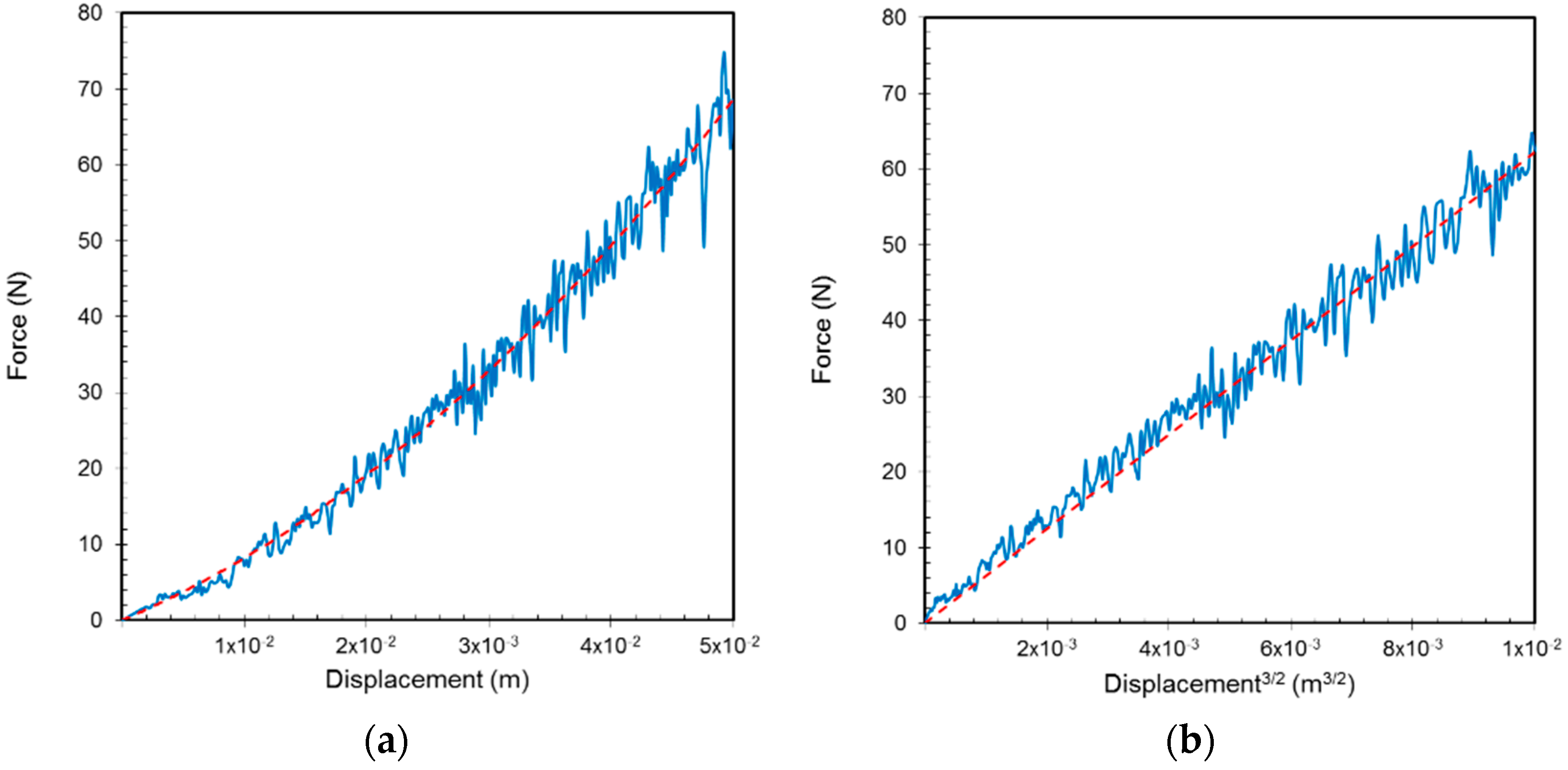
Figure 8a presents the normal contact force as a function of displacement calculated from the simulations using the disorder model with a spring constant of 200 Nm−1. Although this involved a smaller number of beads, the data were a closer fit to a Hertzian response (Figure 8b), but with greater fluctuations of the force. As mentioned above, these fluctuations normally would be removed with an artificial dissipation term, but in this validation example, it is noteworthy that, as expected, disordered structures increased the amplitude of the perturbation. Using Equation (1) and assuming that υ = 0.25, the Young’s modulus was calculated to be 12.4 kPa.
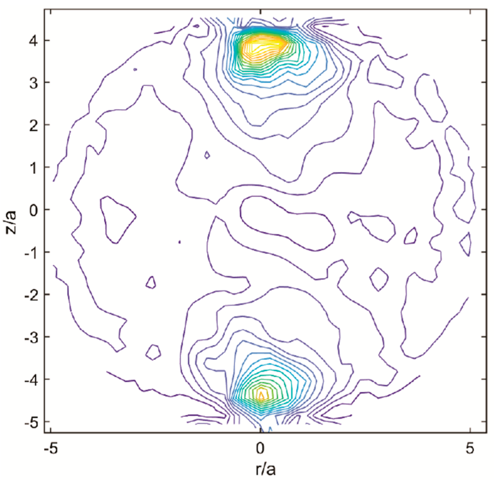
Figure 9 presents the contours of the calculated sub-surface shear stresses, for which due to the random location of the beads, the pattern was not similar in form to that of the cubic lattice cell model. However, the maximum value was also found at a depth of about 0.5a below the surface, which was similar to the cubic lattice model.
3.2. Viscoelastic Spherical Particles
3.2.1. Cubic Lattice Cell Model
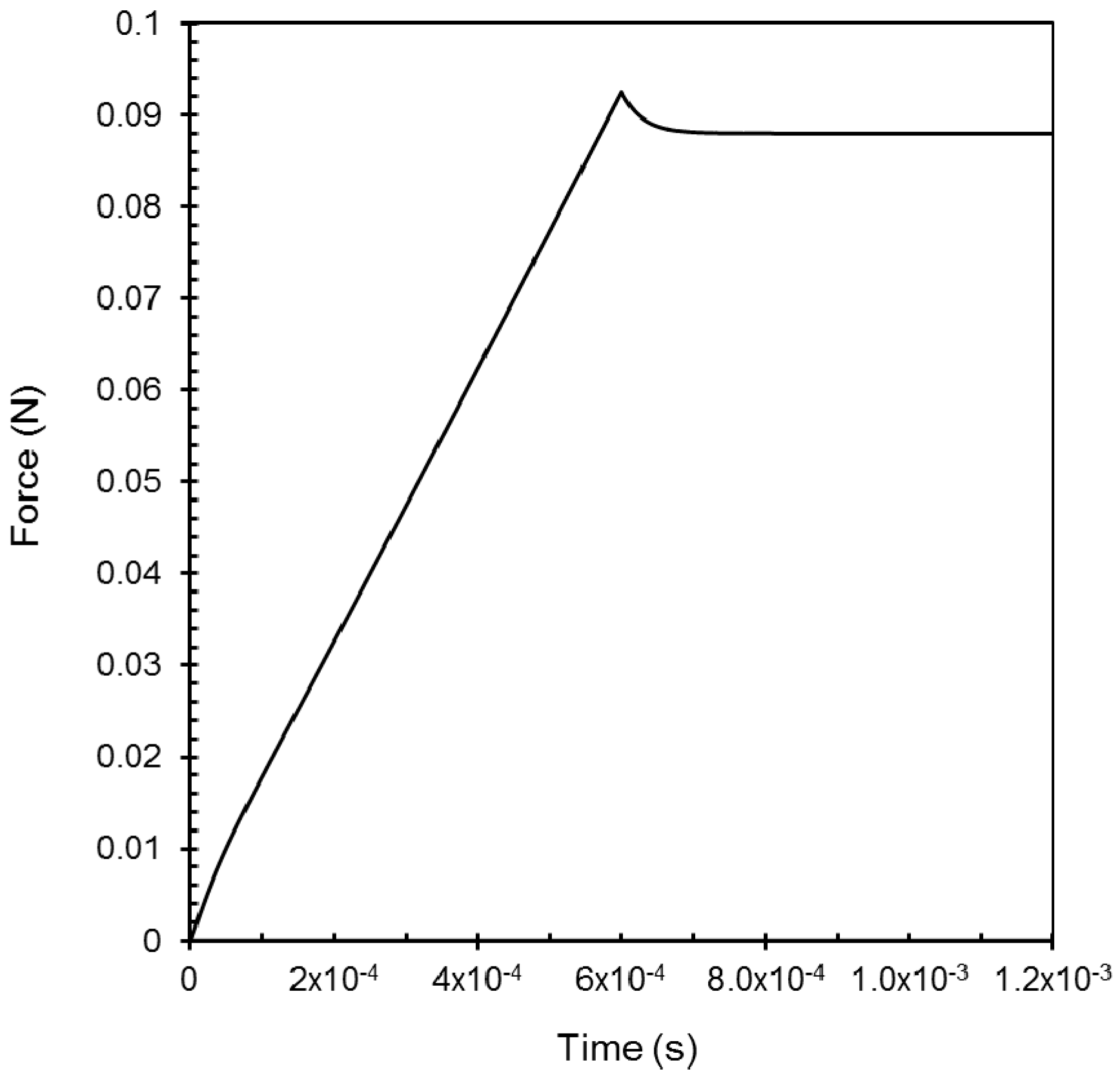
Figure 10 presents the contact force as a function of time during compression and relaxation calculated from the simulations of a viscoelastic spherical model based on the cubic lattice cell during compression with a spring constant of 200 Nm−1 and a dashpot constant of 10−6 Nm−1 s. The force and displacement data were fitted to Equation (2) in order to obtain the value of A, and hence Young’s modulus using Equation (1). It was found to be 36.8 MPa, which was slightly less than that for the elastic particle.
An analysis of the force relaxation after compression was performed using a previous method for experimental compression of an agarose micro-particle [35]. Instantaneous (, corresponding to t = 0) and long-time (, corresponding to t = ∞) elastic moduli were then calculated. The values were found to be = 54 MPa and = 34 MPa. The Hertzian Young’s modulus was close to the calculated relaxed value. The relaxation times are = 0.49 s and = 4.6 × 10⁻⁵ s.
3.2.2. Disorder Model
Figure 11 presents the simulated contact force as a function of time for a viscoelastic spherical particle based on the disorder model with a spring constant of 200 Nm−1 and a dashpot constant of 10−6 Nm−1 s. The force and displacement data were fitted to Equation (2) in order to obtain the value of A, from which the Young’s modulus was obtained using Equation (1) as 112 KPa, which was greater than the calculated value for the elastic particle.
An analysis of the force relaxation after compression was performed using the procedure used for the cubic lattice model. The elastic modulus values were found to be = 203 KPa and = 200 KPa. The Hertzian Young’s modulus was less than the calculated relaxed value, indicating that the force was not fully relaxed after compression. The relaxation time = 0.82 s and = 2.83 × 10⁻⁵ s. It is noteworthy that since the dashpot accounted for the physical viscosity of the material, artificial dissipation was not necessary in these examples.
3.3. Application of the Elastic Disorder Model: Hard Core-Soft Shell and Soft Core-Hard Shell Spherical Particles under Compression
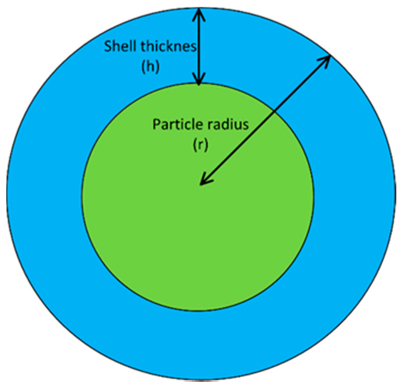
In this section, we consider spherical inhomogeneous particles composed of a hard core-softer shell (HC-SS) and a soft core-harder shell (SC-HS). The models were based on a disorder lattice with 6065 beads. The beads were connected with springs to their neighbours. The hard regions of the particles were modelled using a larger spring constant than that for the soft part. The ratios of shell thickness, h, and the particle radius, r, were set to be 0.5, 0.2, and 0.05. A visualization of the shell thickness and particle radius is presented in Figure 12. A small artificial damping force (1−10 Nm−1.s) was added to the beads, which was proportional to the relative velocity of the beads, in order to damp the kinetic energy from the system and obtain a smoother compression force. Two parallel solid planes were positioned on the surface of the particle in order to simulate diametric compression, as described in the previous section. Using Equation (1) and assuming that υ = 0.25, the Young’s modulus was calculated for each case.
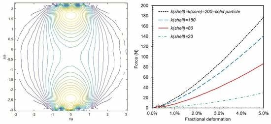
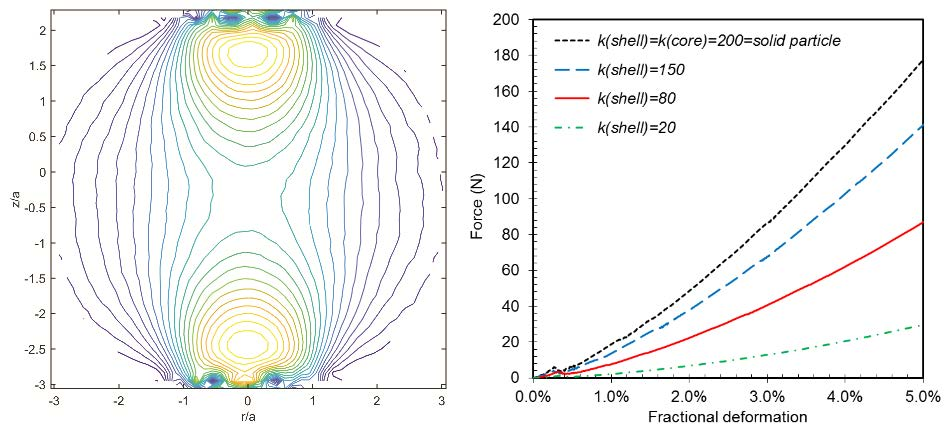
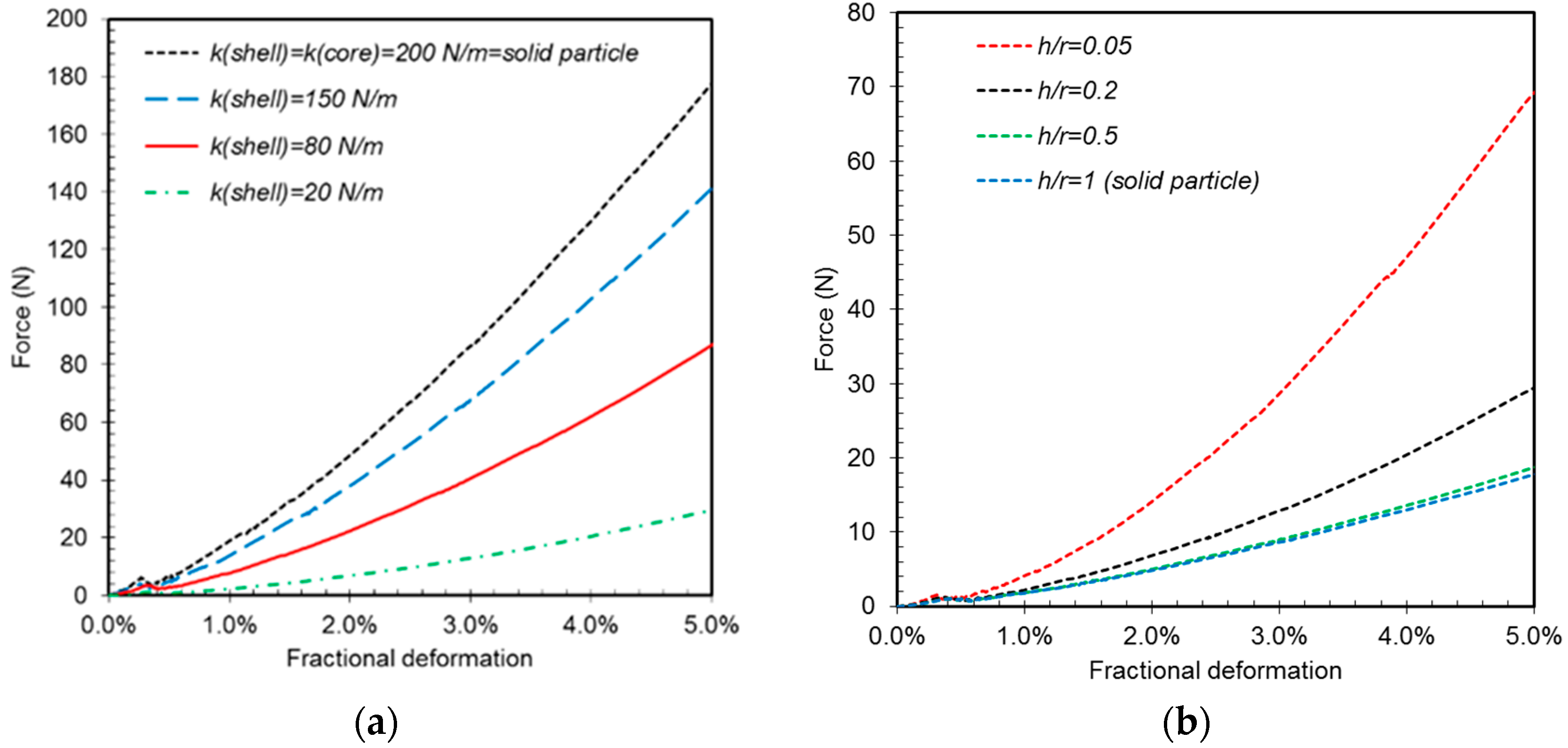
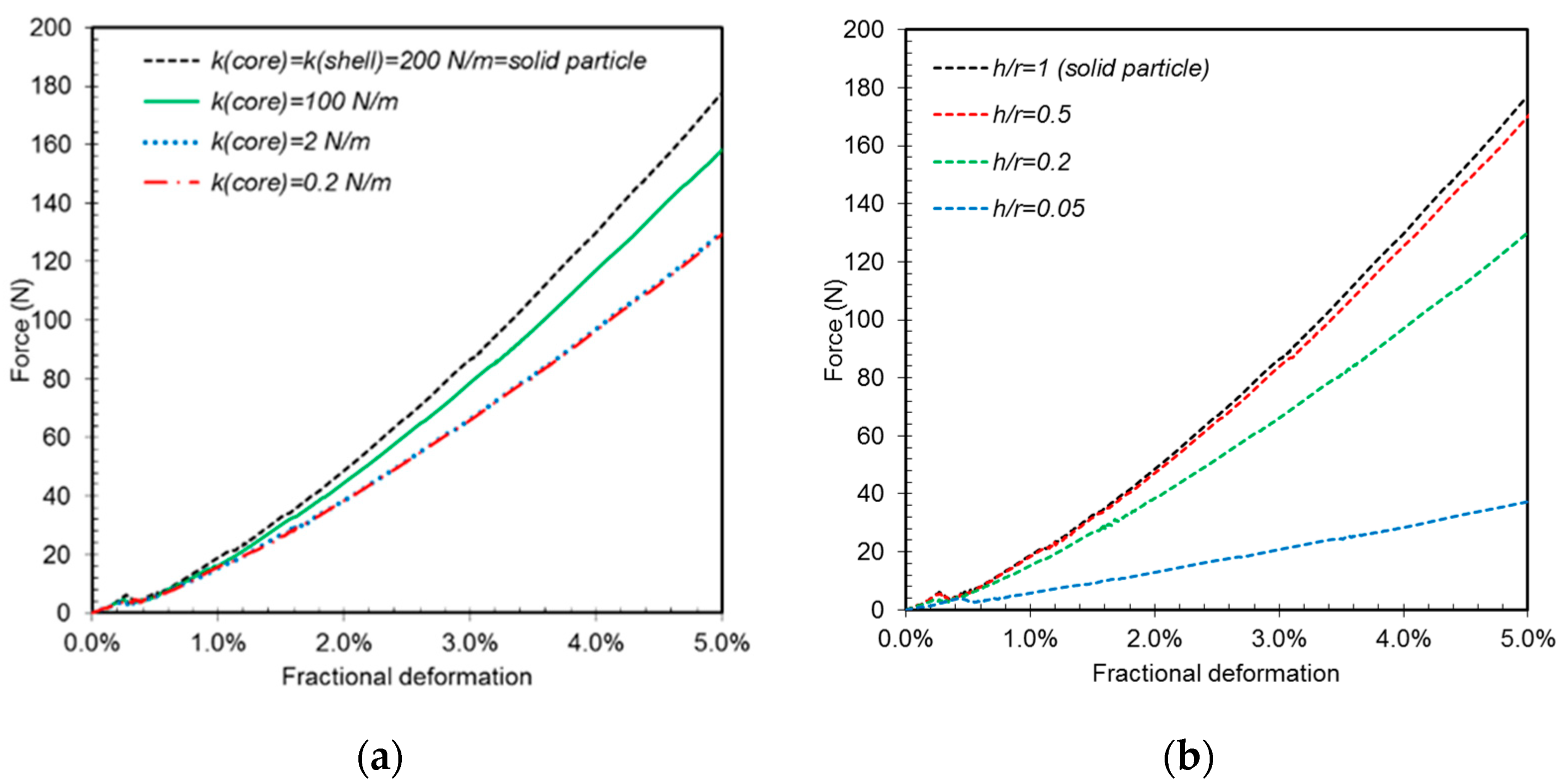
Figure 13 presents the force as a function of fractional deformation (δ/2r) of HC-SS particles with different values of kcore and h/r. Figure 14 presents the force as a function of fractional deformation (δ/2r) of SC-HS particles with different values of kshell and h/r. The force profiles in Figure 13 and Figure 14 can be compared with experimental data to simplify theoretical equations for small deformation e.g. for microcapsules [36].
By comparing Figure 13a and Figure 14a, for the deformation up to 5%, it may be seen that the change in kshell affected the deformation force more significantly than the change in kcore. Figure 13a shows that by reducing kshell from 200 to 20 Nm−1, the deformation force is now just about 11% of the initial value; while in Figure 14a, by reducing Icore from 200 to 0.2 Nm−1, the force now is about 67% of the initial value. Thus, at small deformations, the compression load is mainly absorbed by the shell.
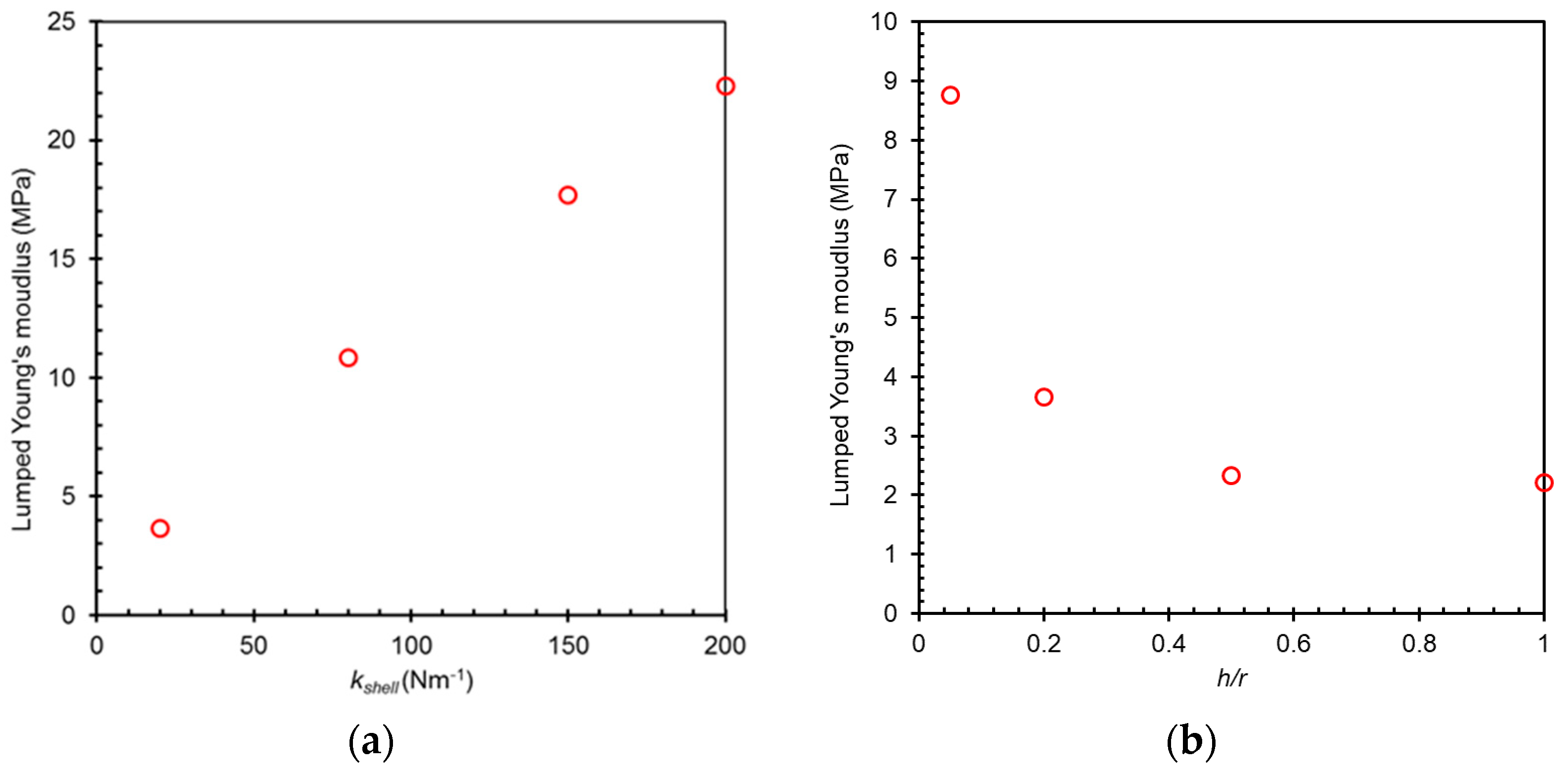
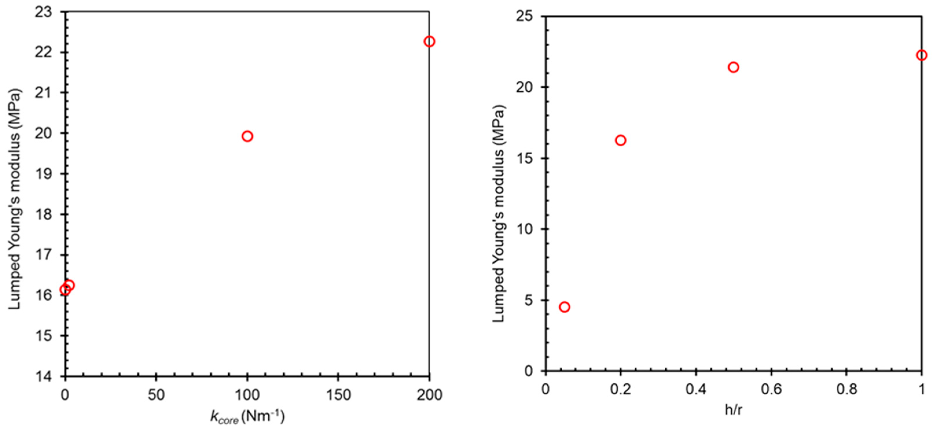
Increasing the h/r ratio from 0.05 to 0.2 changed the deformation force more significantly than increasing the h/r ratio from 0.2 to 1, as presented in Figure 13b and Figure 14b for the deformation up to 5%. Increasing the h/r ratio from 0.5 to 1 did not change the force significantly. Moreover, it may be seen from Figure 15b and Figure 16b that changing the h/r ratio from 0.5 to 1 did not change the lumped Young’s modulus significantly. In these cases, the h/r ratio of 0.5 could be considered as a cut-off ratio where there would be no significant change to the modulus.
Based on the results, a lumped Young’s modulus could be calculated using Equation (1), which represented the equivalent Young’s modulus the particle would have if it were homogeneous. Figure 15 and Figure 16 present the lumped Young’s moduli of HC-SS and SC-HS particles as a function of kshell and kcore, respectively, and as a function of the h/r ratio. As expected, with increasing values of kshell or kcore, the Young’s modulus increases for HC-SS and SC-HS particles, respectively. For the HC-SS particle, increasing the h/r ratio decreased the Young’s modulus, while for the SC-HS particle, it increased the value.
4. Conclusions
It has been demonstrated that the LSM could accurately represent the deformation, including the associated sub-surface stress fields, not only for elastic particles, but also for viscoelastic particles when linear springs were substituted with KV bonds. The disorder model was computationally more efficient than that based on a cubic lattice cell and led to a more refined definition of particle shape. Although only spherical particles were investigated in the current study, the approach is readily applicable to more complex shapes of the type that are often encountered in the pharmaceutical sector. The proposed technique could be employed, within a particle-based multiphysics model such as DMP, to model mechanical inhomogeneity, for example the softening of a particle immersed in water could be modelled by coupling the Young’s modulus with the diffusion coefficient. It could also be extended to non-linear elastic deformation, plastic deformation, and fracture by introducing non-linear springs, friction elements, and springs of limited extensibility. For example, the fracture strength is of particular interest for encapsulates.
If compared with gluing DEM particles together to model different shapes, the proposed technique provided not only accurate contact stresses, but also the stresses within the particle. The disadvantage, however, was in the greater computational cost. However, it was considerably more convenient to implement than discrete finite elements, which require more complex material models. The proposed approach could also be adopted to develop effective interaction laws for inhomogeneous systems in DEM simulations to reduce the computational cost. It would also be possible to incorporate LSM particles in a DEM simulation.
Author Contributions
Conceptualization, I.H.S., A.A., and M.J.A.; methodology, I.H.S., A.A., and M.J.A.; software, I.H.S.; validation, I.H.S.; writing, original draft preparation, I.H.S; writing, review and editing, I.H.S., A.A. and M.J.A.; funding acquisition, A.A. and M.J.A. All authors read and agreed to the published version of the manuscript.
Funding
This research was funded by Engineering and Physical Sciences Research Council, Grant Number EP/M02959X/1.
Acknowledgments
The computations described in this paper were performed using the University of Birmingham’s BlueBEAR HPC service, which provides a High Performance Computing service to the University’s research community. See http://www.birmingham.ac.uk/bear for more details.
Conflicts of Interest
The authors declare no conflict of interest.
Nomenclature
| a | contact radius |
| API | Active Pharmaceutical Ingredients |
| b | dashpot constant |
| δ | relative displacement |
| rate of displacement | |
| DEM | Discrete Element Method |
| DMP | Discrete Multiphysics |
| E | Young’s modulus |
| F | force |
| F(r) | force (diametric compression) |
| FE | viscoelastic normal contact force |
| FH | force (Hertz theory) |
| FKV | force (Kelvin–Voigt model) |
| h | shell thickness |
| HC-SS | hard core-softer shell |
| k | spring constant |
| KV | Kelvin–Voigt |
| l | length of an edge of the cell |
| LSM | Lattice Spring Model |
| m | mass |
| r | radius |
| rb-Ri | distance from the bead to the compression plane |
| Ri | position of the compression plane |
| σ1, σ3 | principal stresses |
| S | specified force constant |
| SC-HS | soft core-harder shell |
| υ | Poisson’s ratio |
| X | distance from equilibrium position |
References
- Alian, M.; Ein-Mozaffari, F.; Upreti, S.R. Analysis of the mixing of solid particles in a plowshare mixer via discrete element method (DEM). Powder Technol. 2015, 274, 77–87. [Google Scholar] [CrossRef]
- Ketterhagen, W.R.; am Ende, M.T.; Hancock, B.C. Process modeling in the pharmaceutical industry using the discrete element method. J. Pharm. Sci. 2009, 98, 442–470. [Google Scholar] [CrossRef] [PubMed]
- Yang, J.; Wu, C.-Y.; Adams, M. DEM analysis of the effect of particle–wall impact on the dispersion performance in carrier-based dry powder inhalers. Int. J. Pharm. 2015, 487, 32–38. [Google Scholar] [CrossRef] [PubMed] [Green Version]
- Lu, G.; Third, J.; Müller, C. Discrete element models for non-spherical particle systems: From theoretical developments to applications. Chem. Eng. Sci. 2015, 127, 425–465. [Google Scholar] [CrossRef]
- Garg, S.; Pant, M. Meshfree methods: A comprehensive review of applications. Int. J. Comput. Methods 2018, 15, 1830001. [Google Scholar] [CrossRef]
- Alexiadis, A. A smoothed particle hydrodynamics and coarse-grained molecular dynamics hybrid technique for modelling elastic particles and breakable capsules under various flow conditions. Int. J. Numer. Methods Eng. 2014, 100, 713–719. [Google Scholar] [CrossRef]
- Alexiadis, A. The discrete multi-hybrid system for the simulation of solid-liquid flows. PLoS ONE 2015, 10, e0124678. [Google Scholar] [CrossRef] [Green Version]
- Ariane, M.; Allouche, M.H.; Bussone, M.; Giacosa, F.; Bernard, F.; Barigou, M.; Alexiadis, A. Discrete multi-physics: A mesh-free model of blood flow in flexible biological valve including solid aggregate formation. PLoS ONE 2017, 12, e0174795. [Google Scholar] [CrossRef] [Green Version]
- Ariane, M.; Allouche, M.H.; Bussone, M.; Giacosa, F.; Bernard, F.; Barigou, M.; Alexiadis, A. Modelling and simulation of flow and agglomeration in deep veins valves using discrete multi physics. Comput. Biol. Med. 2017, 89, 96–103. [Google Scholar] [CrossRef]
- Ariane, M.; Vigolo, D.; Brill, A.; Nash, F.G.B.; Barigou, M.; Alexiadis, A. Using Discrete Multi-Physics for studying the dynamics of emboli in flexible venous valves. Comput. Fluids 2018, 166, 57–63. [Google Scholar] [CrossRef]
- Alexiadis, A.; Ghraybeh, S.; Qiao, G. Natural convection and solidification of phase-change materials in circular pipes: A SPH approach. Comput. Mater. Sci. 2018, 150, 475–483. [Google Scholar] [CrossRef]
- Alexiadis, A. A new framework for modelling the dynamics and the breakage of capsules, vesicles and cells in fluid flow. Procedia IUTAM 2015, 16, 80–88. [Google Scholar] [CrossRef] [Green Version]
- Rahmat, A.; Barigou, M.; Alexiadis, A. Deformation and rupture of compound cells under shear: A discrete multiphysics study. Phys. Fluids 2019, 31, 051903. [Google Scholar] [CrossRef]
- Rahmat, A.; Barigou, M.; Alexiadis, A. Numerical simulation of dissolution of solid particles in fluid flow using the SPH method. Int. J. Numer. Methods Heath Fluid Flow 2019. [Google Scholar] [CrossRef]
- O’Brien, G.S. Discrete visco-elastic lattice methods for seismic wave propagation. Geophys. Res. Lett. 2008, 35. [Google Scholar] [CrossRef]
- Paul, J.; Romeis, S.; Tomas, J.; Peukert, W. A review of models for single particle compression and their application to silica microspheres. Adv. Powder Technol. 2014, 25, 136–153. [Google Scholar] [CrossRef]
- Kuo-Kang, L. Deformation behaviour of soft particles: A review. J. Phys. D Appl. Phys. 2006, 39, R189. [Google Scholar]
- Bakhshian, S.; Sahimi, M. Computer simulation of the effect of deformation on the morphology and flow properties of porous media. Phys. Rev. E 2016, 94, 042903. [Google Scholar]
- Hertz, H. Ueber die Berührung fester elastischer Körper. J. Reine Angew. Math. 1882, 1882, 156–171. [Google Scholar]
- Mook, W.M.; Nowak, J.D.; Perrey, C.R.; Carter, C.B.; Mukherjee, R.; Girshick, S.L.; Gerberich, W.W. Compressive stress effects on nanoparticle modulus and fracture. Phys. Rev. B 2007, 75, 214112. [Google Scholar] [CrossRef] [Green Version]
- Brilliantov, N.V.; Spahn, F.; Hertzsch, J.M.; Pöschel, T. Model for collisions in granular gases. Phys. Rev. E 1996, 53, 5382–5392. [Google Scholar] [CrossRef] [PubMed] [Green Version]
- Schwager, T.; Pöschel, T. Coefficient of restitution for viscoelastic spheres: The effect of delayed recovery. Phys. Rev. E 2008, 78, 051304. [Google Scholar] [CrossRef] [PubMed] [Green Version]
- Zheng, Q.J.; Zhu, H.P.; Yu, A.B. Finite element analysis of the contact forces between a viscoelastic sphere and rigid plane. Powder Technol. 2012, 26, 130–142. [Google Scholar] [CrossRef]
- Kuwabara, G.; Kono, K. Restitution Coefficient in a Collision between Two Spheres. Jpn. J. Appl. Phys. 1987, 26, 1230–1233. [Google Scholar] [CrossRef]
- Plimpton, S. Fast Parallel Algorithms for Short-Range Molecular Dynamics. J. Comput. Phys. 1995, 117, 1–19. [Google Scholar] [CrossRef] [Green Version]
- Ladd, A.J.; Kinney, J.H.; Breunig, T.M. Deformation and failure in cellular materials. Phys. Rev. E 1997, 55, 3271. [Google Scholar] [CrossRef]
- Kot, M.; Nagahashi, H.; Szymczak, P. Elastic moduli of simple mass spring models. Vis. Comput. 2015, 31, 1339–1350. [Google Scholar] [CrossRef]
- Geuzaine, C.; Remacle, J.-F. Gmsh: A 3-D finite element mesh generator with built-in pre- and post-processing facilities. Int. J. Numer. Methods Eng. 2009, 79, 1309–1331. [Google Scholar] [CrossRef]
- Kelchner, C.L.; Plimpton, S.; Hamilton, J. Dislocation nucleation and defect structure during surface indentation. Phys. Rev. B 1998, 58, 11085. [Google Scholar] [CrossRef]
- Nguyen, S. Generalized Kelvin model for micro-cracked viscoelastic materials. Eng. Fract. Mech. 2014, 127, 226–234. [Google Scholar] [CrossRef]
- Chen, H.; Lin, E.; Liu, Y. A novel Volume-Compensated Particle method for 2D elasticity and plasticity analysis. Int. J. Solids Struct. 2014, 51, 1819–1833. [Google Scholar] [CrossRef] [Green Version]
- Thompson, A.P.; Plimpton, S.J.; Mattson, W. General formulation of pressure and stress tensor for arbitrary many-body interaction potentials under periodic boundary conditions. J. Chem. Phys. 2009, 131, 154107. [Google Scholar] [CrossRef] [PubMed] [Green Version]
- Johnson, K.L. Contact Mechanics; Cambridge University Press: Cambridge, UK, 1987. [Google Scholar]
- Lee, S.C.; Ren, N. The Subsurface Stress Field Created by Three-Dimensionally Rough Bodies in Contact with Traction. Tribol. Trans. 1994, 37, 615–621. [Google Scholar] [CrossRef]
- Yan, Y.; Zhang, Z.; Stokes, J.R.; Zhou, Q.Z.; Ma, G.H.; Adams, M.J. Mechanical characterization of agarose micro-particles with a narrow size distribution. Powder Technol. 2009, 192, 122–130. [Google Scholar] [CrossRef]
- Butt, H.-J.; Cappella, B.; Kappl, M. Force measurements with the atomic force microscope: Technique, interpretation and applications. Surf. Sci. Rep. 2005, 59, 1–152. [Google Scholar] [CrossRef] [Green Version]
Figure 1.
Two particles connected by a spring and a dashpot in parallel.

Figure 2.
Comparison of the displacement calculated from the simulation and the analytical solution, i.e., Equation (4).
Figure 2.
Comparison of the displacement calculated from the simulation and the analytical solution, i.e., Equation (4).

Figure 3.
Response of the system depicted in Figure 1 to a constant force, which is removed after 6 s. The blue line is the displacement calculated from the simulation, and the red line is calculated using Simulink.
Figure 3.
Response of the system depicted in Figure 1 to a constant force, which is removed after 6 s. The blue line is the displacement calculated from the simulation, and the red line is calculated using Simulink.

Figure 4.
Response of the system depicted in Figure 1 to a sinusoidal loading force. The lines are the displacements calculated from the simulation, and the points are calculated using Simulink.
Figure 4.
Response of the system depicted in Figure 1 to a sinusoidal loading force. The lines are the displacements calculated from the simulation, and the points are calculated using Simulink.

Figure 5.
(a) Visualisation of a spherical particle between two parallel compression planes, which are represented by red lines; (b) an elementary cell of a cubic lattice.
Figure 5.
(a) Visualisation of a spherical particle between two parallel compression planes, which are represented by red lines; (b) an elementary cell of a cubic lattice.

Figure 6.
(a) Contact force as a function of displacement; (b) contact force as a function of displacement3/2. Both were calculated from the simulations of an elastic spherical particle based on the cubic lattice cell model. The dashed lines are the best fits of the data to the Hertz theory.
Figure 6.
(a) Contact force as a function of displacement; (b) contact force as a function of displacement3/2. Both were calculated from the simulations of an elastic spherical particle based on the cubic lattice cell model. The dashed lines are the best fits of the data to the Hertz theory.

Figure 7.
Contours of the sub-surface shear stresses estimated from the simulations using the cubic lattice cell.
Figure 7.
Contours of the sub-surface shear stresses estimated from the simulations using the cubic lattice cell.

Figure 8.
(a) Contact force as a function of displacement; (b) contact force as a function of displacement3/2. Both were calculated from the simulations of an elastic spherical particle based on the disorder model. The dashed lines are the fits of the simulated data to the Hertz theory.
Figure 8.
(a) Contact force as a function of displacement; (b) contact force as a function of displacement3/2. Both were calculated from the simulations of an elastic spherical particle based on the disorder model. The dashed lines are the fits of the simulated data to the Hertz theory.

Figure 9.
Contours of maximum shear stress beneath the particle surface estimated from the simulations of the particle based on the disorder model.
Figure 9.
Contours of maximum shear stress beneath the particle surface estimated from the simulations of the particle based on the disorder model.

Figure 10.
Contact force as a function of time during compression and relaxation calculated from the simulations of the viscoelastic spherical particle based on the cubic lattice cell model.
Figure 10.
Contact force as a function of time during compression and relaxation calculated from the simulations of the viscoelastic spherical particle based on the cubic lattice cell model.

Figure 11.
Contact force as a function of time during compression and relaxation calculated from the simulations of the viscoelastic spherical particle based on the disorder model.
Figure 11.
Contact force as a function of time during compression and relaxation calculated from the simulations of the viscoelastic spherical particle based on the disorder model.

Figure 12.
Illustration of shell thickness (h) and particle radius (r).

Figure 13.
(a) The force as a function of fractional deformation (δ/2r) of HC-SS particles (h/r = 0.2 and different kshell) and a hard solid particle (kshell = kcore = 200 Nm−1). (b) The force as a function of fractional deformation (δ/2r) of HC-SS particles (kcore = 200 Nm−1 and kshell = 20 Nm−1) with different values of h/r and a soft solid particle (h/r = 1, kcore = kshell = 20 Nm−1).

Figure 14.
(a) The force as a function of fractional deformation (δ/2r) of SC-HS particles (h/r = 0.2 and different kcore) and a hard solid particle (kcore = kshell). (b) The force as a function of fractional deformation of SC-HS particles (kcore = 2 Nm−1 kshell = 200 Nm−1) with different values of h/r and a hard solid particle (h/r = 1, kcore = kshell = 200 Nm−1).

Figure 15.
(a) Lumped Young’s modulus of HC-SS particles of Figure 12a as a function of kshell. (b) Lumped Young’s modulus of HC-SS particles of Figure 12b as a function of h/r.


© 2020 by the authors. Licensee MDPI, Basel, Switzerland. This article is an open access article distributed under the terms and conditions of the Creative Commons Attribution (CC BY) license (http://creativecommons.org/licenses/by/4.0/).
Share and Cite
MDPI and ACS Style
Sahputra, I.H.; Alexiadis, A.; Adams, M.J. A Coarse Grained Model for Viscoelastic Solids in Discrete Multiphysics Simulations. ChemEngineering 2020, 4, 30. https://0-doi-org.brum.beds.ac.uk/10.3390/chemengineering4020030
AMA Style
Sahputra IH, Alexiadis A, Adams MJ. A Coarse Grained Model for Viscoelastic Solids in Discrete Multiphysics Simulations. ChemEngineering. 2020; 4(2):30. https://0-doi-org.brum.beds.ac.uk/10.3390/chemengineering4020030
Chicago/Turabian StyleSahputra, Iwan H., Alessio Alexiadis, and Michael J. Adams. 2020. "A Coarse Grained Model for Viscoelastic Solids in Discrete Multiphysics Simulations" ChemEngineering 4, no. 2: 30. https://0-doi-org.brum.beds.ac.uk/10.3390/chemengineering4020030