Visible and Near Infrared Image Fusion Using Base Tone Compression and Detail Transform Fusion


School of Electronic and Electrical Engineering, Kyungpook National University, 80 Daehakro, Bukgu, Daegu 41566, Korea
*
Author to whom correspondence should be addressed.
Chemosensors 2022, 10(4), 124; https://0-doi-org.brum.beds.ac.uk/10.3390/chemosensors10040124
Submission received: 30 January 2022
/
Revised: 11 March 2022
/
Accepted: 22 March 2022
/
Published: 25 March 2022
(This article belongs to the Section Analytical Methods, Instrumentation and Miniaturization)
Abstract
:This study aims to develop a spatial dual-sensor module for acquiring visible and near-infrared images in the same space without time shifting and to synthesize the captured images. The proposed method synthesizes visible and near-infrared images using contourlet transform, principal component analysis, and iCAM06, while the blending method uses color information in a visible image and detailed information in an infrared image. The contourlet transform obtains detailed information and can decompose an image into directional images, making it better in obtaining detailed information than decomposition algorithms. The global tone information is enhanced by iCAM06, which is used for high-dynamic range imaging. The result of the blended images shows a clear appearance through both the compressed tone information of the visible image and the details of the infrared image.
Keywords:
image fusion; near-infrared image; contourlet transform; iCAM06; HDR; PCA fusion; homography1. Introduction
Visible and near-infrared (NIR) images have been used in various ways for surveillance systems. Surveillance sensors usually block infrared light using a hot mirror filter or an infrared cut filter in the daytime. This hot mirror filter is then removed at night. During daytime, infrared light saturates an image and distorts the color information because of too much light. Furthermore, the infrared scene is an achromatic image. During nighttime, infrared light can capture objects in dark areas through the thermal radiation emitted by these objects at night [1]. NIR scenes contain detailed information that is not expressed in visible scenes during daytime because the NIR has a stronger permeability to particles (e.g., in foggy weather) than the visible images [2]. Thus, the image visibility can be improved by visible and NIR image synthesis. The synthesis of visible and NIR images is performed to obtain complementary information.
To synthesize visible and NIR images, the simultaneous capturing of visible and NIR scenes is an important step in visible and NIR image fusion. Therefore, many camera devices are used to capture the visible and NIR scenes. A device can be made in two main ways: using one camera sensor and using two camera sensors. One camera sensor should be used to capture the visible and NIR scenes using a visible cut filter and an IR cut filter in front of the camera lens. However, a time-shifting problem occurs when one sensor is used when utilizing two filters. Thus, two spatially aligned camera sensor modules using a beam splitter are necessary to prevent time-shifting errors. The beam splitter divides visible and NIR rays. Each divided visible and NIR ray enters the two camera sensors to simultaneously acquire visible and NIR images. However, when two camera sensors are used, the problem of image position movement and alignment mismatch may occur. The image alignment method using homography can be used to solve the position-shifting error [3].
In the next step, a method for synthesizing the images of two different bands taken according to the characteristics is required. Many methods have been developed for visible and NIR image fusion. These techniques include the Laplacian–Gaussian pyramid and local entropy fusion algorithm [4], latent low-rank representation fusion algorithm [5], dense fuse deep learning algorithm [6], and Laplacian pyramid PCA fusion [7]. The Laplacian–Gaussian pyramid and local entropy fusion algorithm is used to synthesize visible and NIR images by transmitting the maximum information of the local entropy. It is based on the multi-resolution decomposition by the Laplacian–Gaussian pyramid, and multiple resolution images are fused by each layer using the local entropy fusion method. This algorithm is good to preserve detailed information in an NIR image, but the color expression is exaggerated compared to an input visible image.
The latent low-rank representation fusion algorithm (Lat-LRR) decomposes images into low-rank (i.e., global structure) and saliency (i.e., local structure) parts. The low-rank parts are fused by the weighted-average method to preserve detailed information, while the saliency parts are fused by the sum strategy. The resulting image is obtained by combining the fused low-rank and saliency parts. This algorithm is also good for preserving detailed information, but has noise in the result images. Moreover, this algorithm does not contain any color compensation part; thus, it would be unnatural for the result images to adapt color information where the color information is taken in the visible image.
Dense fuse is a deep learning-based approach of fusing visible and infrared images. This deep learning network consists of convolutional and fusion layers and dense blocks. A dense block connects the output of each layer to every other layer; thus, the input layer information is cascaded to the next layer. The process of deep learning fusion attempts to obtain more useful features from the source images in the encoding process. These layers, which are processed by the encoding process, are fused through two strategies, namely, the additional and -norm strategies. The fused image is reconstructed by a decoder process. The advantage of a dense block is that it preserves the previous information as long as possible and reduces overfitting. This is called the regularizing effect. Compared to other deep learning fusion methods, this method can preserve more useful information from middle layers and is easy to train. However, the result images are not clearer than those of the previous algorithm fusion methods. Son et al. proposed multi-resolution image decomposition using the Laplacian pyramid and an image fusion technique using the principal component analysis (PCA) [7]. Their method reduces the side effects of synthesis by controlling the image synthesis ratio through the PCA by generating a weight map in a specific local area and synthesis in an unnecessary area.
The proposed method uses contourlet transform [8], PCA fusion [9], and iCAM06 tone compression [10]. Contourlet transform extracts the directional details of visible and NIR images separated by the bilateral filter. The PCA fusion algorithm is utilized to fuse visible and NIR directional details. Meanwhile, the PCA is used to calculate the optimal weight of the visible and NIR directional detailed information. The tone compression of the visible base image is based on iCAM06, which has the main purpose of increasing the local contrast for high-dynamic range (HDR) imaging. In the iCAM06 process, the Stevens effect compensation step improves the contrast of the luminance channel, and the fused image is post-processed by color compensation. The proposed method can solve the unnaturalness of the color with the color information suitable for improved contrast. The fused result images show better details and color naturalness than conventional methods.
2. Related Works
2.1. Image Fusion with Visible and NIR Images
A method for synthesizing the visible and near-infrared images has been extensively studied for decades. Light scattering by fog blurs the image boundaries and reduces the image detail. The image visibility can be improved through a post-image correction method using gamma correction or histogram equalization. However, the improvement performance of these methods is limited because detailed information is not fundamentally included in the input image. To solve this problem, research on the capture and synthesis of near-infrared and visible light images is in progress [11,12,13].
The near-infrared rays corresponding to the wavelength band of 700–1400 nm have a stronger penetrability to fog particles than visible rays. Therefore, a clear and highly visible image can be reproduced by synthesizing near-infrared and visible light images in a foggy or smoky environment. As a representative method, Vanmali et al. composed a weight map by measuring the local contrast, local entropy, and visibility and synthesizing the resulting image through color and sharpness correction after the visible and near-infrared image synthesis [4]. In addition, Son et al. proposed a multi-resolution image decomposition using the Laplacian pyramid and an image fusion technique using the PCA [7].
A PCA-based synthesis is accomplished using the mean weights of and , which are calculated by multiplying the weights in each input image in Equations (1)–(5). is the result of the image synthesis calculated by the PCA synthesis algorithm with the input visible and NIR images (i.e., and , Figure 1 and Equation (5)). The PCA is a method of linearly combining the optimal weights for the data distribution and uses a covariance matrix and the eigenvectors of the data [14]. The covariance matrix is a kind of matrix that can describe how similar the variation of feature pairs ( are, that is, how much feature pairs change together. Equation (1) shows how to organize the covariance matrix. is a covariance matrix; is an eigenvector; and is an eigenvalue. The covariance matrix is composed of an orthogonal matrix of the eigenvector matrix and the diagonal matrix of the eigenvalue.
where is the covariance matrix; is an eigenvector matrix; and is an eigenvalue matrix.
Equations (1) and (2) can be used to calculate the eigenvalues and the corresponding eigenvectors. A matrix of each eigenvector and eigenvalue matrix is calculated in the image PCA fusion algorithm. The biggest eigenvalue and the corresponding eigenvectors are used for the PCA weight calculation. The normalize eigenvectors and these values are the optimal weight for synthesizing the visible and NIR images, as shown in Equations (3) and (4).
where is an eigenvalue; is an eigenvector matrix corresponded by eigenvalue; is an optimal weight of the visible and NIR fusion algorithm; is the sum of the eigenvector matrix; and is an element of the eigenvector matrix.
For the visible and NIR detail image fusion, the PCA is used to analyze the principal components of the data of the collected distribution of the visible and NIR images. The PCA determines the optimal image synthesis ratio coefficient for the visibility and the insufficient areas for the NIR. PCA-based fusion is performed using the optimal weight of and calculated by multiplying the weights of each input image in Equation (5).
where is a result image fused by the visible and NIR images; and are the optimal fusion weights; and and are the input visible and NIR detail images.
2.2. Contourlet Transform
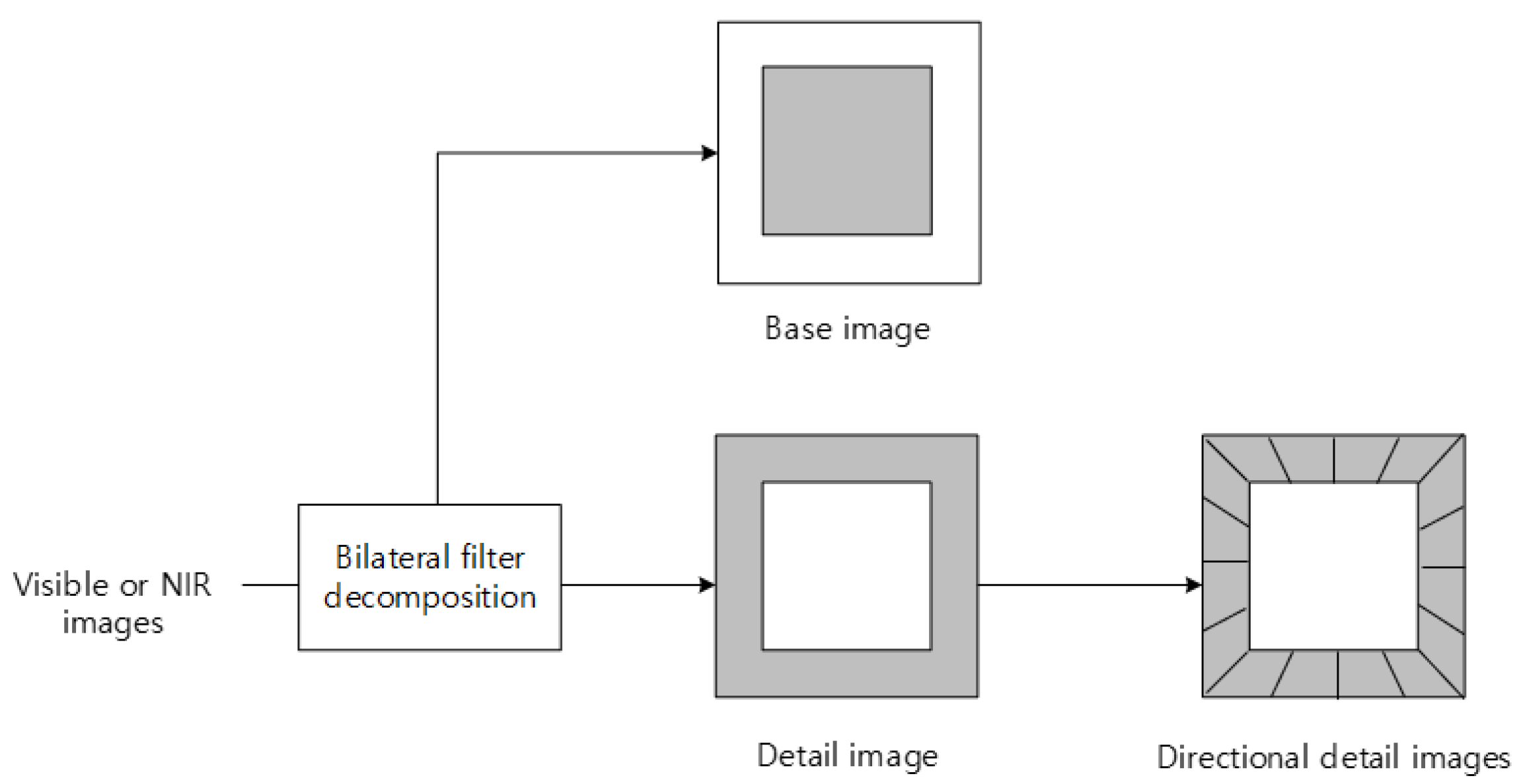
The contourlet transform divides the image by frequency band using a multiscale concept (e.g., two-dimensional wavelet transform), and then uses directional filter banks to obtain the directional information of the images within the divided area. Unlike wavelet transform, the contourlet transform comprises double repeating filters of the Laplacian pyramid and the directional filter bank; hence, it is called a pyramidal directional filter bank [15]. In the wavelet transform, the image information may overlap between high- and low-band channels after down-sampling. However, the Laplacian pyramid can solve this disadvantage of overlapping frequency components by down-sampling in low frequency channels. The directional filter bank is composed of a quincunx filter bank and a shearing operator. The quincunx filter is a horizontal and vertical directions of two channel fan filter. The shearing operator simplifies the sequence samples of images. Directional filters can be effectively implemented through -level binary tree decomposition, which produces subbands with a wedge-shaped frequency division.
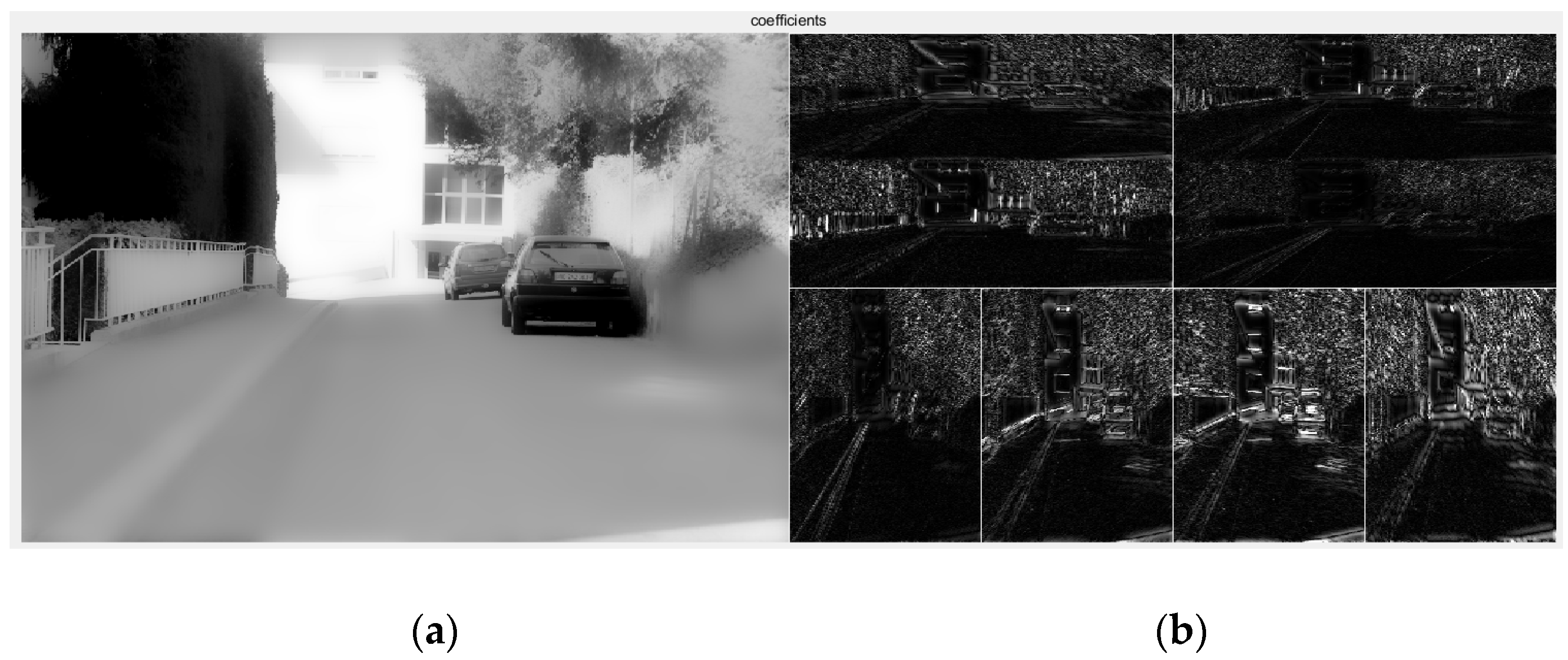
In the iCAM06 process, the base and the detail layers are decomposed into a bilateral filter [10]. The detail layer is decomposed into a directional subband by the directional filter bank used in the contourlet transform. The result image is obtained by combining the tone compression base image and the detail image processed by the PCA fusion algorithm and the Stevens effect from the directional detailed image (Figure 2). Figure 3 depicts the directional detail images and the base image. Contourlet transform can capture smooth contours and corners in all directions.
2.3. Image Align Adjustment
In the proposed method using two image sensors, the alignments of the visible and NIR images did not match. Therefore, the homography theory [3] is used to align the visible and NIR images. Before calculating the homography matrix, the key points and descriptors must be obtained using the scale-invariant feature transform (SIFT) algorithm [16]. The SIFT algorithm mainly has four parts: scale-space extrema detection, keypoint localization, orientation assignment, and keypoint and descriptor. After getting the key points and the descriptors using the SIFT algorithm, they should be calculated to obtain feature matching. Feature matching refers to pairing similar objects by comparing the keypoints and descriptors in two different images. The result of finding the keypoint pair with the highest similarity is stored in feature matching. This pair of keypoints (i.e., visible and NIR keypoints) is used to calculate the homography matrix, which can match the visible and NIR images.
Homography produces the corresponding projection points when one plane projects to another. These corresponding points exhibit a constant transformation relationship, known as homography, which is one of the easiest ways to align different images. Homography requires the calculation of a 3 × 3 homography matrix. The homography matrix, H, exists only once and is calculated using ground and image coordinates. The homography theory generally requires only four corresponding points. Equation (6) is an example of a homography matrix equation:
where is the reference image (e.g., visible keypoint sets); is the target image (e.g., NIR keypoint sets); and is the homography matrix.
Equation (7) is a formula expressed by the matrix of Equation (6):
where and are the reference image coordinates, and and are the target-image coordinates. The through the 3 × 3 matrix is a homography matrix that can align visible images with NIR images.
Equations (8) and (9) are the matrix equations obtained from Equation (7):
Dividing the equation of the first row into the equation of the third-row results in a matrix equation, such as Equation (8). Furthermore, dividing the equation of the second row by the equation of the third row, as previously shown, results in a matrix equation like Equation (9). Equations (6)–(9) calculate the matrix equations and are used for the first response point. Homography calculates at least four response points; thus, four calculations must be made, as previously shown. Equations (10) and (11) are the matrix representation of a matrix formula calculated using Equations (8) and (9):
Given that two matrix equations are generated per response point, the matrix size of Equation (10) is 8 × 9. and are the target image coordinates corresponding to the first response point, while and are the target image coordinates corresponding to the fourth response point. The matrix equation can be represented using matrix in Equation (10) and in Equation (11). Equation (11) is represented in the homography coordinates as a one-dimensional matrix. in Equations (7) and (11) is always 1. Equations (8)–(11) can be expressed as shown in Equation (12):
where matrix represents the 1st–4th corresponding feature points between the reference and target images. The homography matrix, , can be calculated by applying the singular value decomposition of matrix . Figure 4 depicts an example of the aligned visible and NIR images using the homography theory.
3. Proposed Method
3.1. Dual Sensor-Capturing System
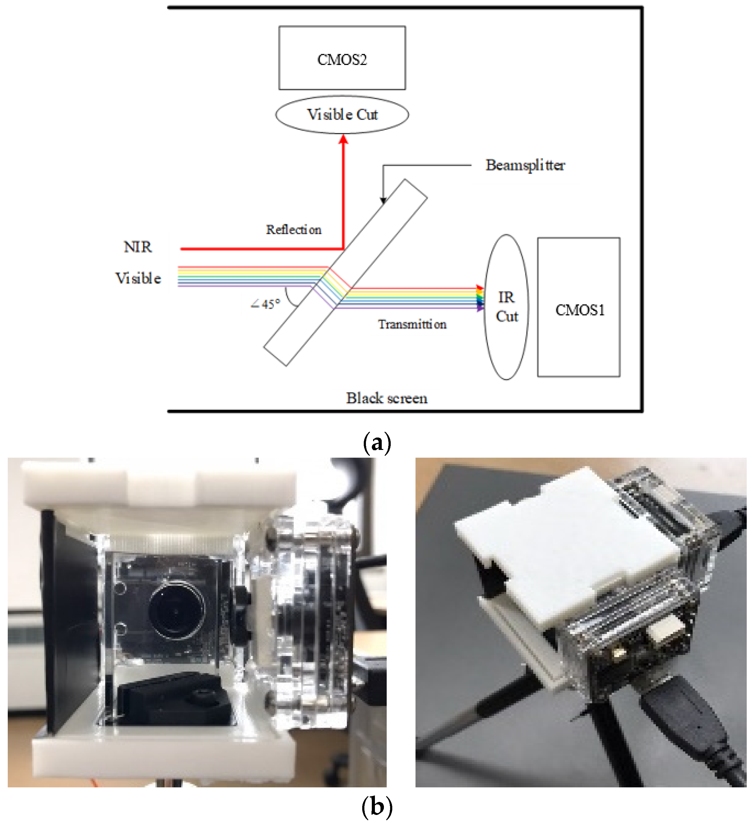
The proposed method suggests a new camera device comprising two complementary metal oxide semiconductor wideband cameras and a beam splitter (Figure 5) to acquire visible and NIR images without a time-shifting error. A two-CMOS camera device (oCam-5CRO-U) (WITHROBOT, Seoul, Korea) module is used because a time-shifting error occurs if only one camera sensor is used to take visible and NIR images. The CMOS broadband camera can take a photograph in a spectral band from the visible to NIR rays. The CMOS camera has an autofocus function and a simple and low-cost camera sensor. Therefore, it can be easily set up to capture visible and NIR scenes.
A beam splitter is set up between the CMOS camera sensors to separately obtain the visible and NIR images using each CMOS camera sensor. The beam splitter divides the visible and NIR rays. Each divided visible and NIR ray enters the two CMOS camera sensors to simultaneously obtain the visible and NIR images. For a camera module, the OmniVision OV5640 CMOS image sensors (OmniVision Technologies, Santa Clara, CA, USA) were used. The Camera’s allowable wavelength is around from 400 to 1000 nm. The visible cut filter’s blocking wavelength is around from 450 to 625 nm and the IR cut filter’s cut off wavelength range is 710 nm. These camera and filters’ wavelength are specified in Table 1. The beam splitter is a 35 mm × 35 mm, 30R/70T, 45° Hot Mirror VIS plate beam splitter (Edmund Optics, Barrington, IL, USA), which allows visible light to pass through and reflect infrared light. Table 2 presents the light transmittance and reflectance of the beam splitter and the wavelength.
In Figure 5, each of the visible and IR cut filter is in front of the CMOS camera sensor to filter the visible and NIR rays. The beam splitter splits rays to visible and NIR rays and indicates spatial division. The advantage of spatial division over time division is that during image capture, the object is not in a different position and reflects the same scene. A camera module box is built to prevent light scattering. The side in the direction of the camera is made of black walls to prevent the reflection of light. The CMOS camera devices are arranged to vertically take photographs of the NIR image based on the beam splitter and of the visible image in the direction of the beam splitter. This device displays a position-shifting error; therefore, the proposed method uses the homography theory to align both visible and NIR images. Figure 6 illustrates an example of the visible and NIR images taken by the proposed beam splitter camera device.
Figure 6a displays some over-saturated phenomena and low saturation of the visible image. Compared to the visible image, the NIR image shows clear details both in the sky and in the shade. The image in Figure 6b has fewer colors and details in the visible image, but the night NIR image shows better details in the dark area. Therefore, the proposed visible and NIR fusion algorithm must take details from the NIR image and collect color information from the visible image.
3.2. Visible and NIR Image Fusion Algorithm
The proposed algorithm has two different visible and NIR fusion algorithms: a luminance channel fusion algorithm and an XYZ channel fusion algorithm. The luminance channel (L channel) fusion algorithm uses the LAB color space based on iCAM06. The visible and NIR images are converted by the luminance channel in the LAB color space. Moreover, the XYZ channel fusion algorithm is based on iCAM06. Visible and NIR images are converted by the XYZ color space. Figure 7 shows the block diagrams of the entire two algorithms.
3.2.1. Base Layer—Tone Compression
Image visibility can be improved through the method after gamma correction or histogram equalization; however, the improvement performance of this method is limited because details are not included in the input image. As mentioned above, the NIR rays corresponding to the wavelength band of 700 nm to 1400 nm contain more detailed information better than that of visible rays. Therefore, a clear view can be reproduced by synthesizing the visible and NIR images. The NIR image has more detailed information in the shading and overly bright areas; thus, the visible image sharpness can be increased by utilizing the detail area of the NIR image.
The proposed method uses the iCAM06 HDR imaging method to improve the visibility of the visible images. iCAM06 is a tone-mapping algorithm based on the color appearance model, which reproduces the HDR rendering image. The iCAM06 model is extended to a low scotopic level to a photopic bleaching level in the luminance range. The post-adaptation nonlinear compression is a simulation of the photoreceptor response, including cones and rods [17]. Thus, the tone compression output of iCAM06 is a combination of cone and rod response. iCAM06 is based on white point adaptation, photoreceptor response function for tone compression, and various visual effects (e.g., Hunt effect, Bartleson–Breneman effect for color enhancement in the IPT color space, and Stevens effect for detail layer). Moreover, iCAM06 can reproduce the same visual perception across media. Figure 8 depicts a brief flow chart.
In Figure 8, the input visible image color space is converted into an RGB to a XYZ channel. The image decomposition part is that the input image decomposes the base and detail layers. The chromatic adaptation estimates the illuminance and converts the color of an input image into the corresponding colors under a viewing condition. The tone compression operates on the base layers using a combination of cone and rod responses and reduces the image’s dynamic range according to the response of the human visual system. Thus, it performs a good prediction of all available visual data. The image attribute adjustment part enhances the detail layer using the Stevens effect and rearranges the color adjustment of the base layer to change the IPT color space using the Hunt and Bartleson effects. The result output image adds the processed base and detail layer through the iCAM06 process.
The base layer was decomposed by the bilateral filter. The visible base image was processed as a tone compression based on HDR image rendering. The tone-compressed visible base image improved the local contrast, as shown in Figure 7. Two different tone compressions are presented, namely, the luminance channel tone compression shown in Figure 7a and the XYZ channel tone compression shown in Figure 7b. Adding the tone-compressed base image and the detail image processed by the contourlet transform and the PCA fusion algorithm resulted in the proposed radiance map. The difference between the radiance maps of the luminance and XYZ channels was color existence. The combined image of the base and the details of the XYZ channel cannot be expressed as a radiance map. It is called a tone-mapped image.
3.2.2. Detail Layer—Transform Fusion
The bilateral filter is used to decompose the base and detail images. The bilateral filter is a nonlinear filter that reduces noise while preserving edges. The intensity value of each pixel is replaced by a weighted average of the nearby pixel values [18]. This weight is not only associated with the Euclidean distance between the pixel and the neighboring pixels, but also with the difference in the pixel values, which is called radiometric difference. The bilateral filter is applied considering the intensity difference of the surrounding pixels; hence, the edge-preserve effect can be observed. In other words, the detail image is the difference between the original and base images, which is a bilateral filtered image. The detail images decomposed by the bilateral filter in the luminance channel consist of each visible and NIR detail image. In the XYZ channel fusion algorithm, the detail images consist of each XYZ channel, which comprises three detail images of visible and NIR images. The detail visible and NIR images are decomposed by contourlet transform, which directionally decomposes the detail images. Each detailed information should be fused by optimal weight; thus, the optimal weight must be calculated using the PCA fusion algorithm. After the detail layer processing, which is fused by the PCA algorithm with contourlet transform, the details are applied to the Stevens effect to increase the brightness contrast (local perceptual contrast) with the increasing luminance. The detail adjustment is given as Equation (13).
where is a result of the detail processed by the Stevens effect; is the fused detail image processed by the PCA and contourlet transform; and is a factor of luminance-dependent power-function adjustment based on the base layer.
where is decomposed by a bilateral filter; is 20% of the adaptation luminance in the base layer; is the adjustment factor; and is a factor of various luminance-dependent appearance effects to calculate Stevens effect detail enhancement. The details are enhanced to apply the Stevens effect in the detail layer.
3.2.3. Color Compensation and Adjustment
After generating the radiance map in both the luminance and XYZ channel proposed algorithms, color compensation was applied to significantly increase the image’s naturalness and improve its quality. The tone changes through image fusion caused a color distortion due to the changes in the balance of the RGB channels of tone. The ratio of the RGB signals will change, and the color saturation would be reduced.
In the luminance channel, the color compensation was calculated as the ratio of the radiance map and the visible luminance channel. The color signal conversion was necessary in building a uniform perceptual color space and in correlating various appearance attributes. The ratio of color to luminance after tone mapping was applied to the color compensation in the luminance channel fusion algorithm to correct these color defects in tone mapping [19]. The color compensation ratio was calculated by the radiance map and the visible luminance channel images, as given in Equation (15).
where is the color compensation ratio that describes the surrounding brightness variation between the radiance map () and the visible luminance image ().
The color compensation in the LAB color space is given in Equation (16), where is the color compensation ratio given in Equation (15); and are the visible color information in the LAB color space; and and are the compensated chrominance channels. This corrected LAB color space image was converted into an RGB image to obtain the proposed result image of the luminance channel fusion.
In the XYZ channel fusion algorithm, the color adjustment of the result image was processed by the IPT transformation. The base layer image in the XYZ channel fusion was first processed through the chromatic adaptation to estimate the illuminance and convert the input image color into the corresponding colors under a viewing condition [20]. Compared to the luminance channel fusion algorithm, the base layer of the XYZ channel fusion algorithm contained color information. After the base layer was processed by tone compression, it was added to the detail layer, and the primary image fusion was completed. The XYZ channel fusion algorithm did not need the color compensation process.
The tone map image was converted into an IPT uniform relative color space, where I was almost similar to a brightness channel; P is a red–green channel; and T is a blue–yellow channel. In the IPT color space, P and T were enhanced by the Hunt effect predicting a phenomenon, where an increase in the luminance level resulted in a perceived colorfulness given in Equations (17)–(19).
where is the IPT exponent; is a red–green channel; and is a blue–yellow channel.
where and are the enhanced and processed by the Hunt effect, respectively; is a chroma value given in Equation (14); is the IPT exponent given in Equation (10); and I in the IPT color space denotes brightness, which is similar to the image contrast. I increases when the image surround changes from dark to dim to light. This conversion is based on the Bartleson surround adjustment given in Equation (20):
where is an enhanced ; is a brightness channel; and is the exponent of the power function: .
In the proposed XYZ fusion algorithm, was used to enhance . To adapt to the color change according to the increase in the image brightness, the XYZ color space was converted into the IPT color space to apply the Hunt and Bartleson effects. This corrected IPT color space image was then converted into an XYZ image. The converted XYZ image was converted back into an RGB image to obtain the proposed result image of the XYZ channel fusion.
In summary, the color compensation of the luminance channel fusion method uses the ratio between the radiance map and the visible input luminance image and considers tone scaling with the brightness gap. Therefore, in luminance channel fusion, this color compensation complements the color defects. Another proposed XYZ channel fusion method uses the IPT color space to improve colorfulness through the Hunt and Bartleson effects. Therefore, in the XYZ channel fusion, the color adjustment depends on the brightness of the tone-mapped base layer image.
4. Simulation Results
4.1. Computer and Software Specification
The proposed method was implemented on a PC with an Intel i7-7700K processor, 16GB RAM. For photography and image homography alignment, Opencv 4.5.3 version and python 3.8.5 version softwares were used. The visible and NIR image processing was performed using the Windows version of MATLAB R2020a software.
4.2. Visible and NIR Image Fusion Simulation Results
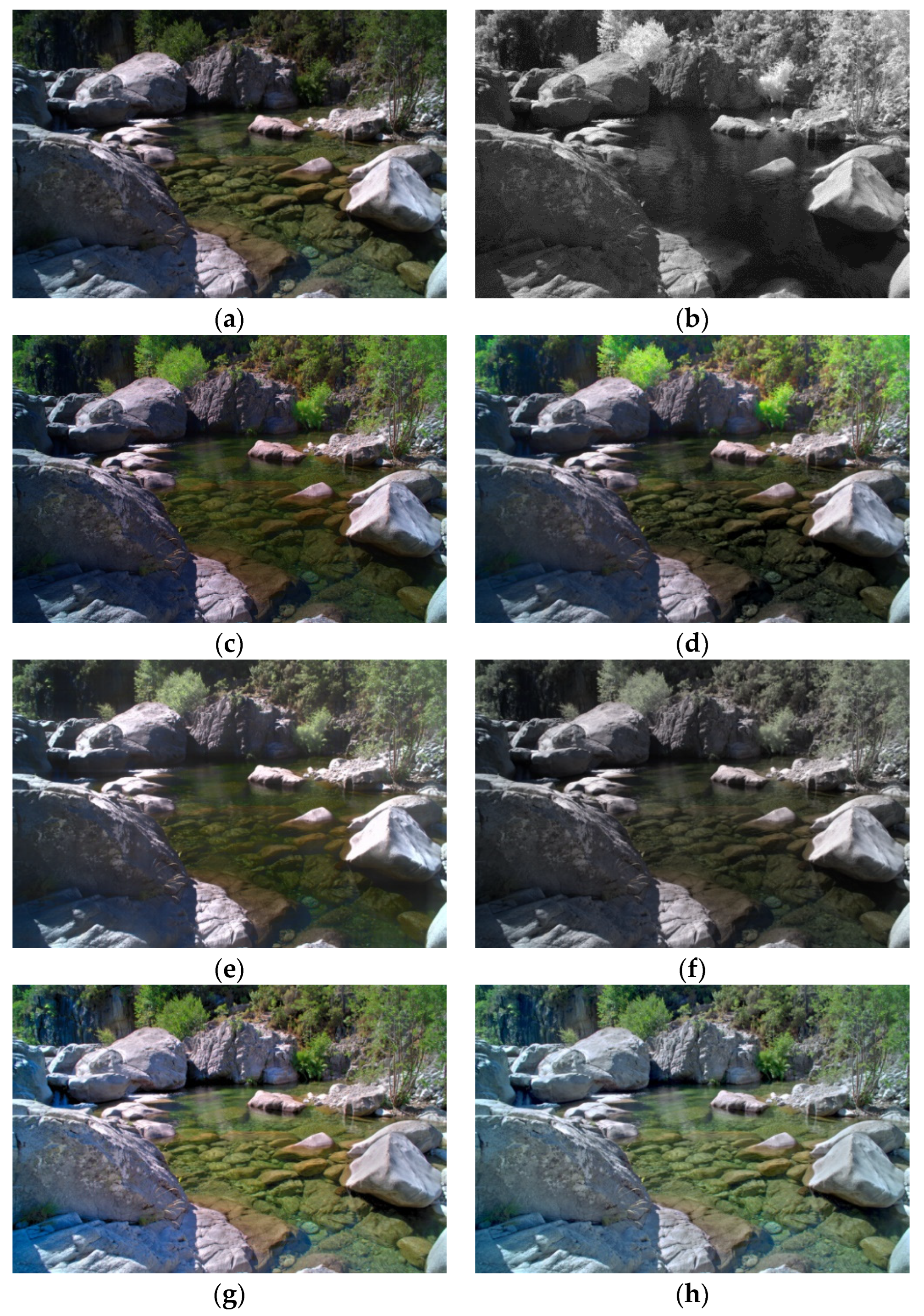
Figure 9, Figure 10, Figure 11, Figure 12, Figure 13 and Figure 14 illustrate comparisons of the conventional visible and NIR image fusion algorithm and the proposed method. The conventional fusion algorithms were the Laplacian entropy fusion [4], Laplacian PCA fusion [7], low-rank fusion [5], and dense fusion [6]. The result image of the low-rank fusion was grayscale; hence, the color component of the visible image was applied to compare the result images on the same line.
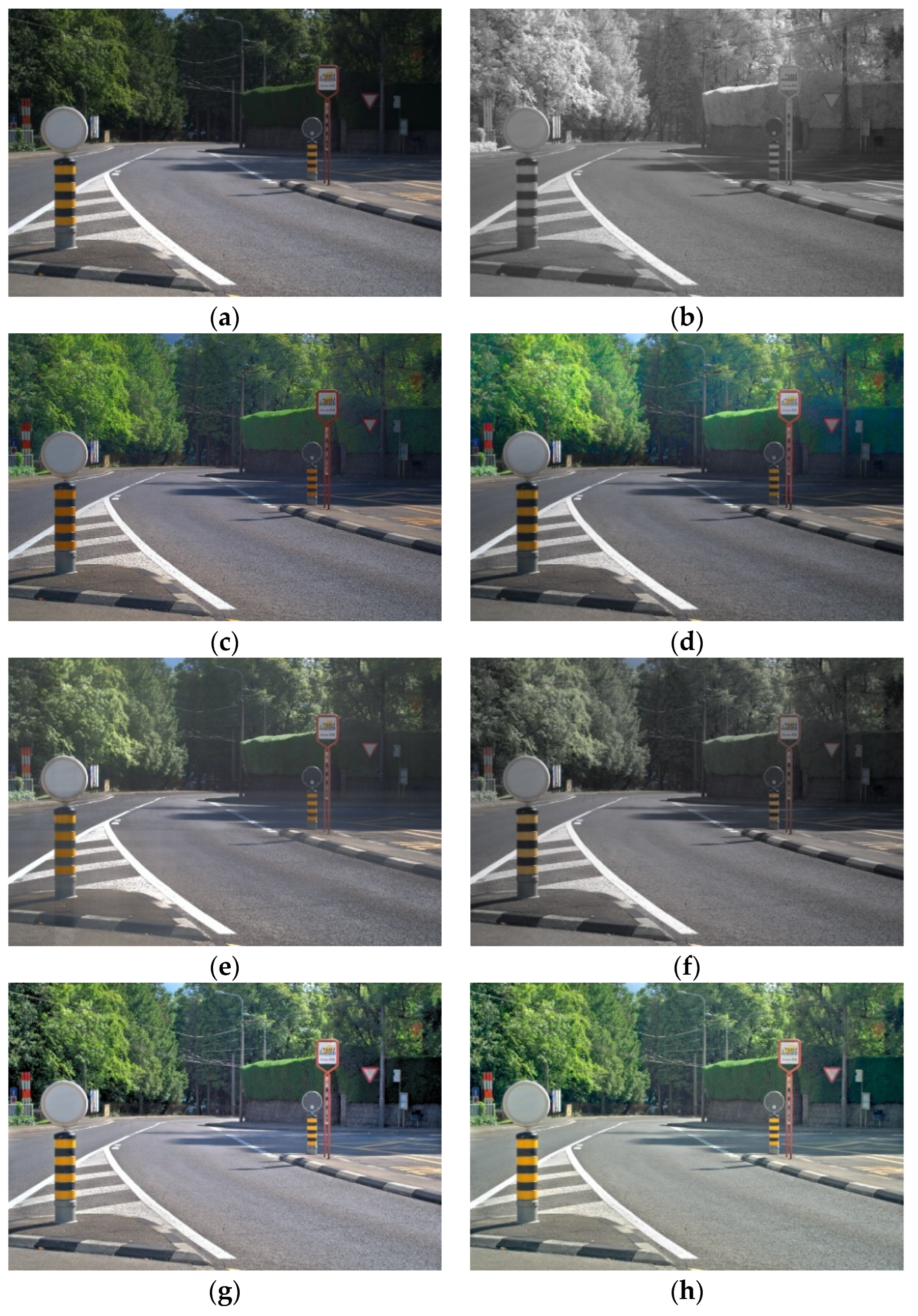
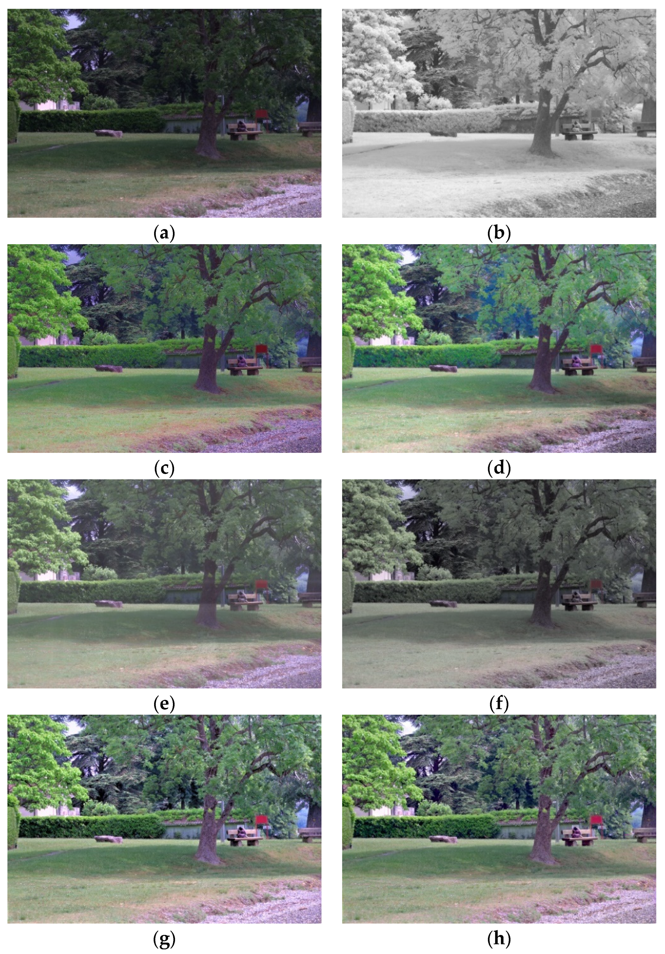
The result images of the low-rank fusion contained noise, while those of the dense fusion exhibited an unnatural color expression. Both result images of the Laplacian entropy fusion and the Laplacian PCA fusion were better detail expressions than the other conventional methods, albeit still being dim and dark in the shading area. The proposed method of the luminance channel showed better details and an improved local contrast. The result images naturally expressed the color of the input image well. The proposed method of the XYZ channel also had better details in the shading area, and the color information was followed by the human visual system. The result image of the proposed methods can be selected according to the conditions of the visible images.
In Figure 9, the tone and detail of the shaded area have been improved, allowing identification of the license plate number. In Figure 10, the low-level tone generated by backlighting was improved (rock area), and the detail of the distant part by the NIR image and the advantages of the water transmission performance by the visible image were well expressed. Therefore, the characteristics of visible and NIR images are well combined and expressed. In Figure 11, the contrast ratio between the luminance of the dark part inside the alley and the luminance of the sky with strong external light was well compressed, greatly improving the object expression performance of the entire image. In Figure 12, it is confirmed that the detail in the distant shaded area of the road was improved. In Figure 13, the color expression of objects is natural and the details of the complicated leaf part are well expressed compared to the existing method. In Figure 14, it is confirmed that the object identification performance for the shaded area between buildings (especially the tree part) is improved.
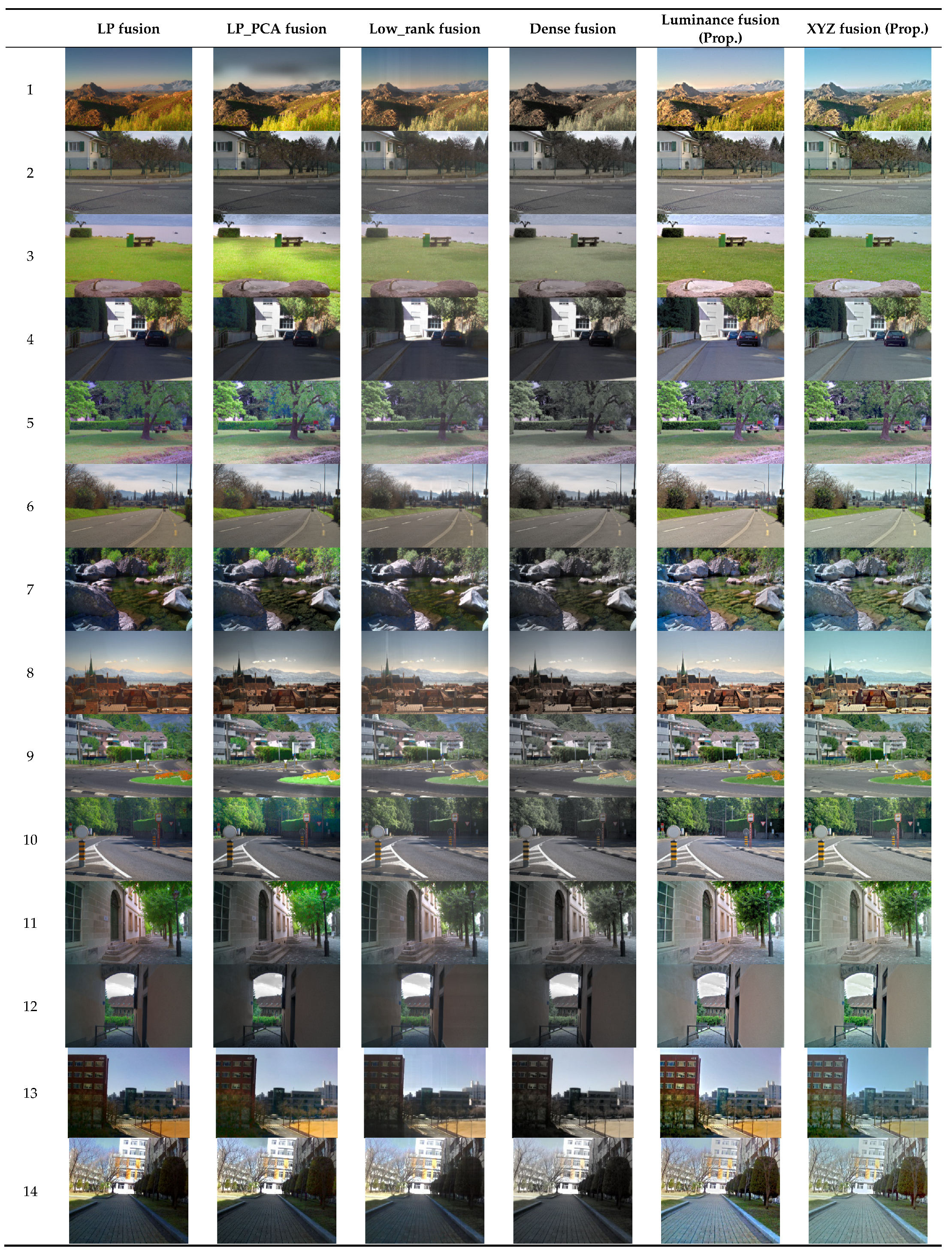
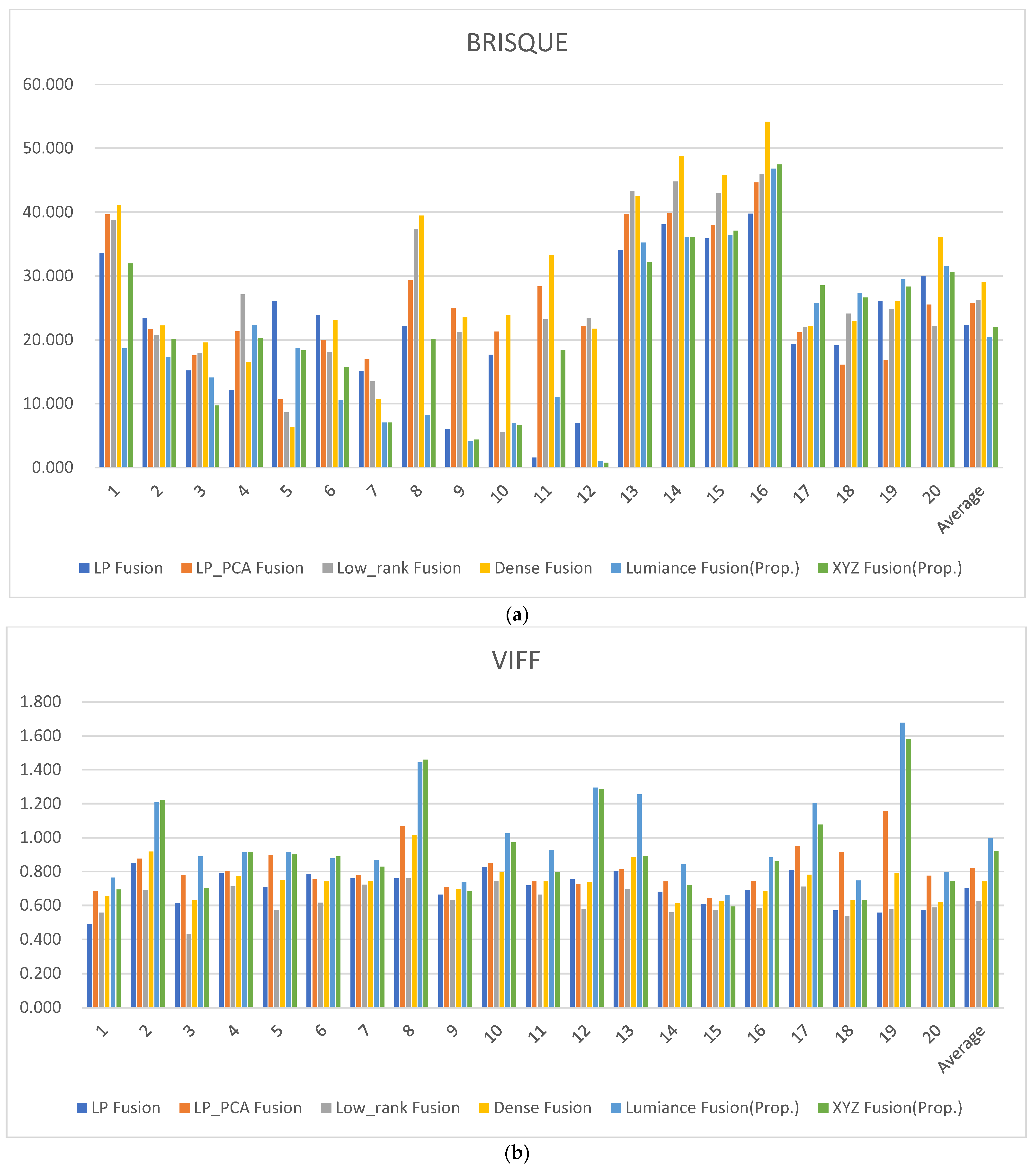
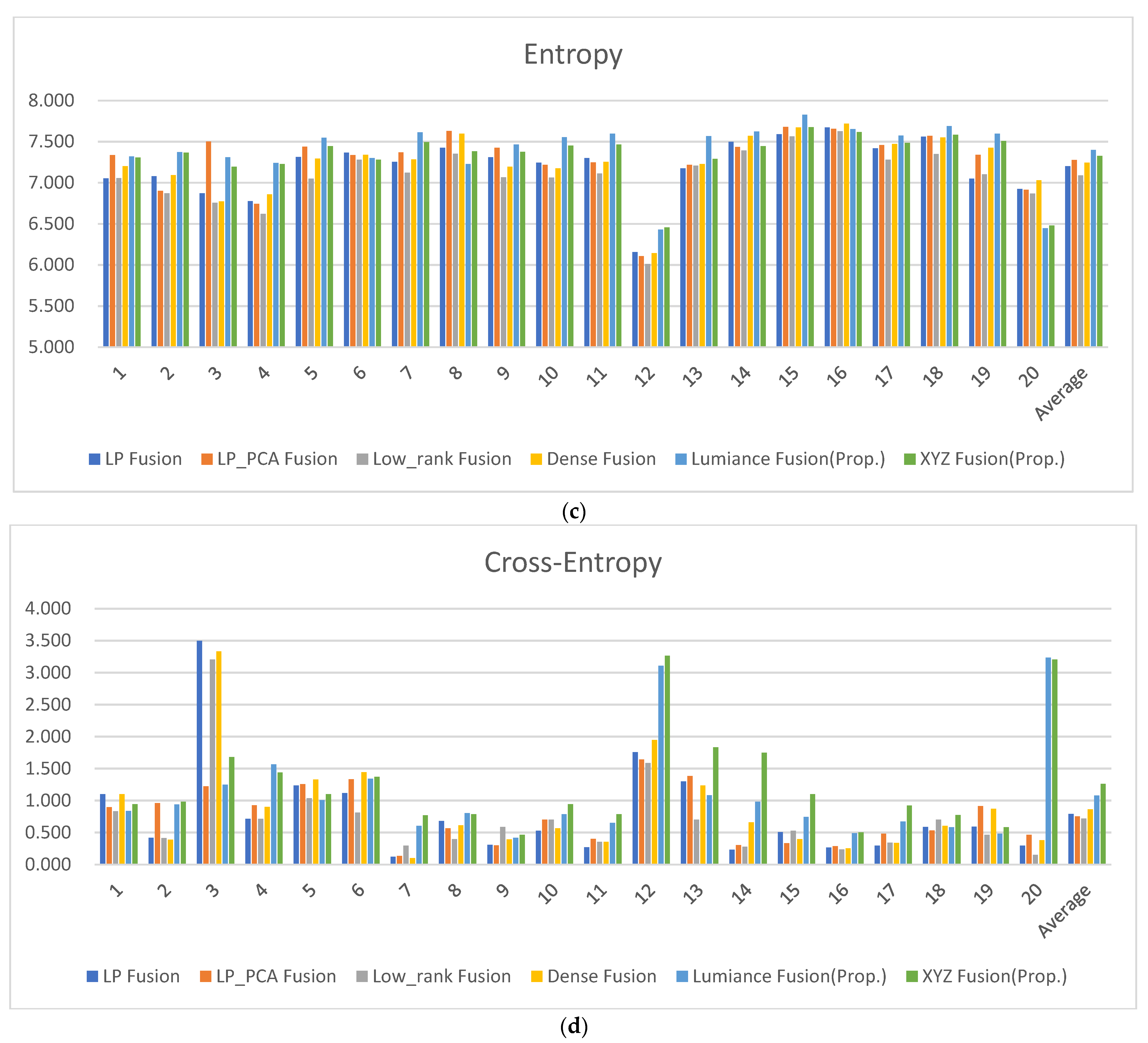
The resulting image values were calculated and presented in Table 3, Table 4, Table 5, Table 6, Table 7, Table 8, Table 9, Table 10 and Table 11 [21]. Figure 15 is a collection of the result images of each method used for metric score comparison. In Table 3, the Blind/Referenceless Image Spatial Quality Evaluator (BRISQUE) is a no-reference image quality metric that utilizes the NSS model framework of local normalized luminance coefficients and quantifies naturalness using the model parameters [22]. The lower the BRISQUE score, the better the image quality. The BRISQUE score average in the luminance and XYZ fusion presents the lowest score (better quality) when compared to the other conventional methods (Table 3, Figure 16a). The visual information fidelity for fusion (VIFF) measures the effective visual information of the fusion in all blocks in each sub-band [23]. VIFF performs the calculation of distortion between the fused image and the source image. Entropy (EN) analysis defines that all fused image data contain more information [24]. The higher the entropy value, the more information the fused image contains, that is, the higher the entropy value, the better the performance of the fusion method. Cross entropy evaluates the similarity of information contents between the fused image and the source image [25]. The higher the cross entropy value, the higher the similarity. In Table 4, Table 5 and Table 6, the higher the value, the better the fused image quality. The luminance fusion method in VIFF and EN scores presents the highest score when compared to the other conventional methods in Figure 16b–d. However, in Cross entropy, the XYZ fusion method presents the highest score.
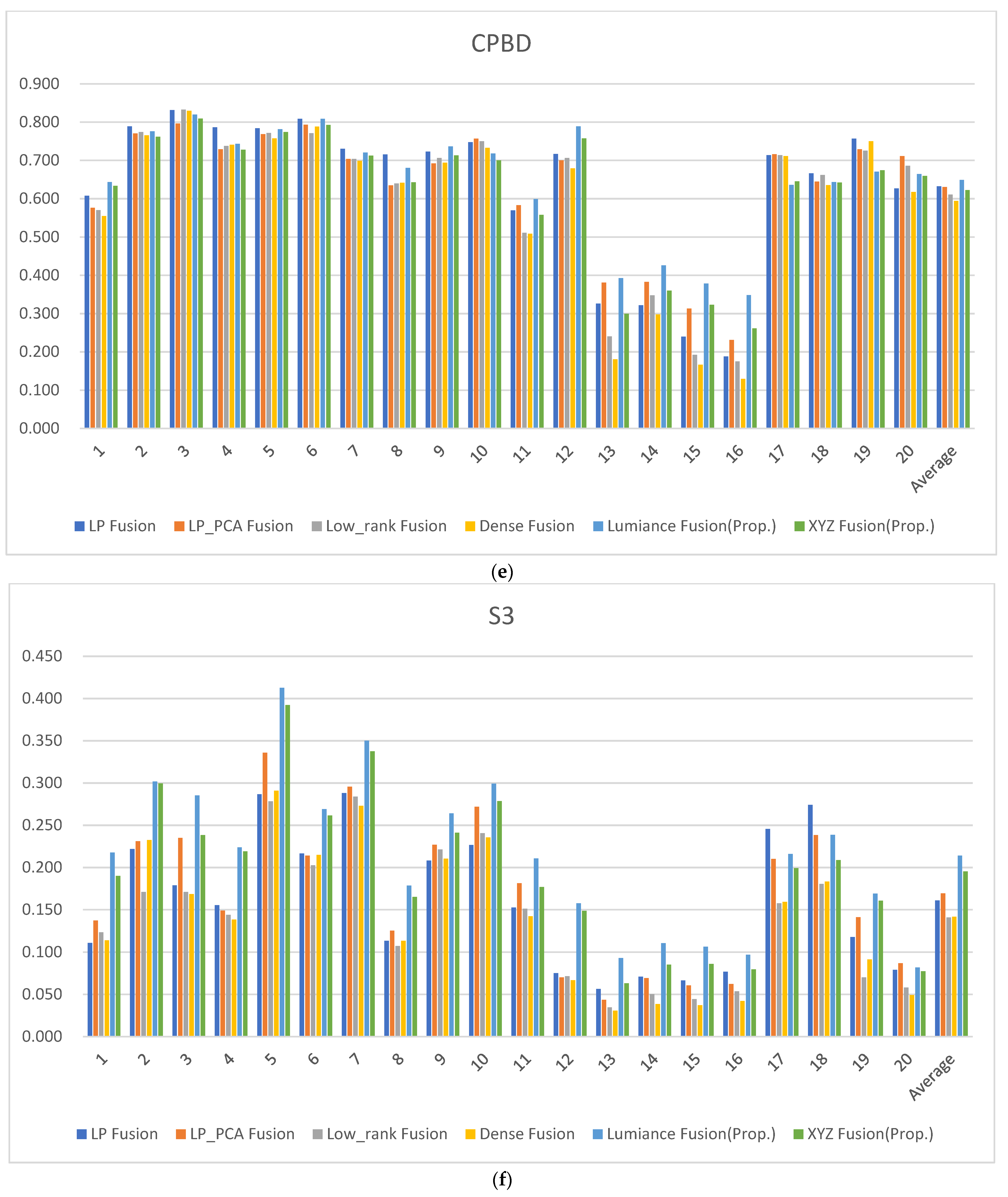
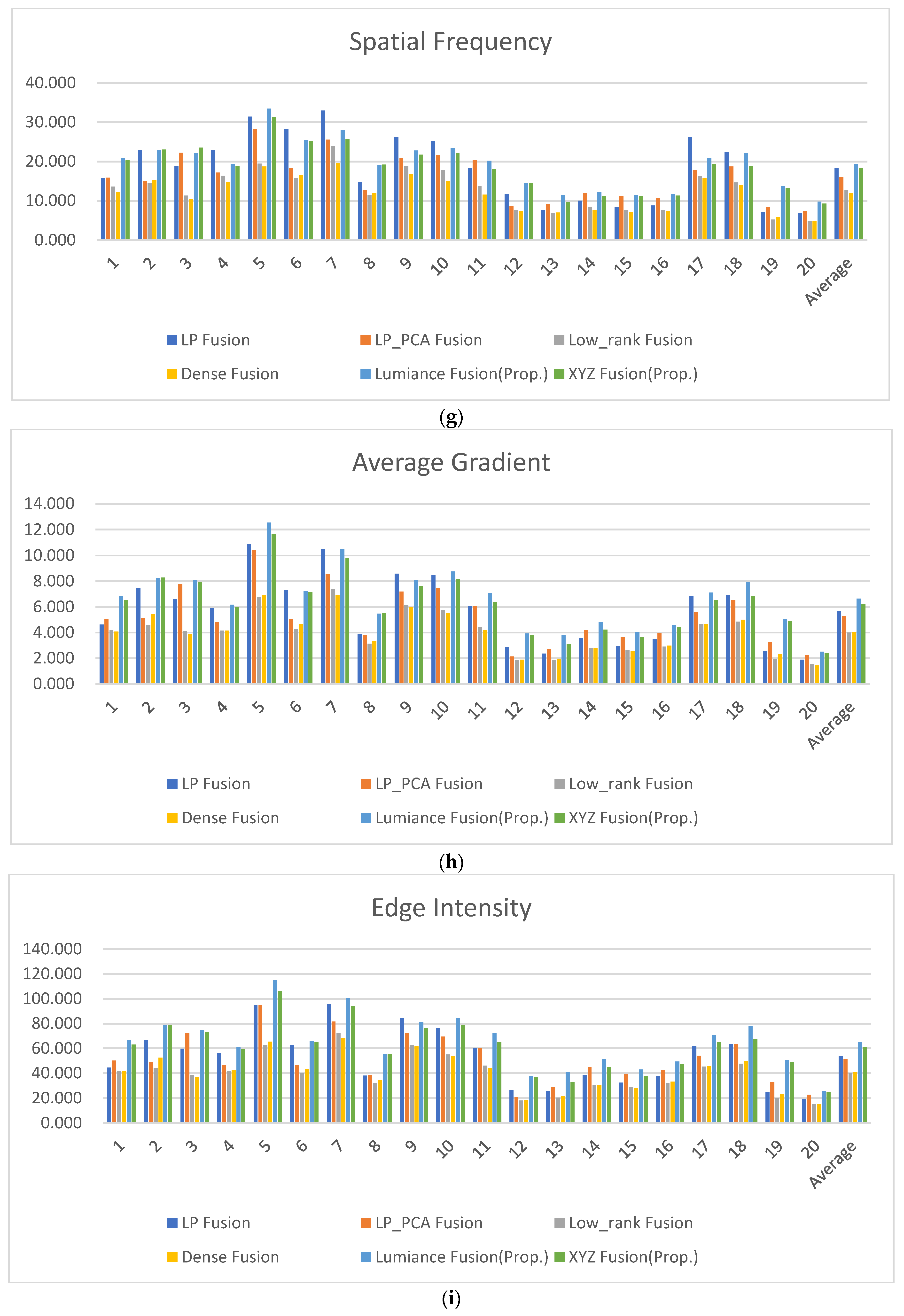
In Table 7, Table 8, Table 9, Table 10 and Table 11, this score represents the sharpness metric. The cumulative probability of blur detection (CPBD) involves the estimation of the probability of detecting blur at the detected edge following the edge detection [26]. The spectral and spatial sharpness (S3) yields a perceived sharpness map, in which larger values represent perceptually sharper areas [27]. The Spatial Frequency (SF) metric can effectively measure the gradient distribution of an image, revealing detail and texture in an image [28]. The higher the SF value of the fused image, the more sensitive and rich the edges and textures are to human perception according to the human visual system. The average gradient (AG) metric quantifies the gradient information in the fused image and reveals detail and textures [29]. The larger the average gradient metric, the more gradient information is contained in the fused image and the better the performance of preserving edge details. The edge intensity (EI) indicates that the higher edge intensity value for an image, the better the image quality and sharpness [30]. The higher the CPBD, S3, SF, AG, EI scores, the better the image sharpness. Figure 16e–i display the scores of the CPBD, S3, SF, AG and EI. Overall, the proposed luminance fusion and XYZ fusion methods show superior scores compared to all other methods; also, the luminance fusion results present a better evaluation scores than the XYZ fusions on average.
5. Discussion
The proposed method’s result images have advantage of better detail expression, local contrast enhancement, and well-expressed color. In Figure 13, the details of complex leaf parts of light and dark areas were well expressed, so the image clarity can be increased without any ambiguity. In addition, the advantages of visible and NIR images with different clear characteristics such as Figure 10 and Figure 11 were well combined and expressed. The underwater details of the visible image and the long-distance details of the NIR image were well expressed together. In Figure 11, the visible image shows no detail of bright clouds in the saturated sky area. On the other hand, the NIR image represents the details of clouds well. Since the existing methods use the light exposure state of the photographed image as it is, only the improvement of the bright sky part is confirmed. However, since the proposed method includes a tone compression method, it shows an improved synthesis result for the insufficiently exposed portion of the input image. Therefore, the proposed method improves the local contrast and sharpness characteristics of the entire image at the same time. In particular, the proposed method can be used in many applications requiring object recognition because it can distinguish objects in a shaded area well in a fused image. The luminance fusion method is judged to have excellent synthesizing effects on the separated luminance components, and the XYZ fusion method enables color expression reflecting the color adaptation of the CAM visual model.
6. Conclusions
In this study, we presented a visible and NIR fusion algorithm and a beam splitter camera device. First, the visible and NIR images were simultaneously acquired using a beam splitter camera device without a time-shift error, and a fusion algorithm was applied with contourlet transform and the PCA fusion algorithm based on iCAM06. The proposed fusion algorithm comprised two methods: synthesizing in the luminance channel and synthesizing in the XYZ channels. In the luminance channel fusion, the only luminance channels of the image were used to generate a radiance map via iCAM06’s tone compression process with contourlet transform and PCA fusion in detail layers. The color compensation was calculated by the ratio of the radiance map and the luminance of the input visible image. The XYZ channel fusion used chromatic adaptation to estimate the illuminance and convert the color of an input image into the corresponding colors under the viewing condition. The tone compression was then processed to reduce the dynamic range of the image according to the cone response of the human visual system. The XYZ NIR detail layer was decomposed through contourlet transformation and fused using the PCA algorithm. The resulting image of the XYZ channel was color-adjusted through the IPT color space conversion. The color adjustment of the basic layer aimed to change the IPT color space using the Hunt and Bartleson effects. The result image of blending the visible and NIR images led to better detailed information and color naturalness when compared to conventional methods. The proposed method can possibly be adapted in real-life applications, for example, camera visual quality enhancement or camera sensors for vehicles and automobiles.
Author Contributions
Conceptualization, S.-H.L.; methodology, S.-H.L. and D.-M.S.; software, D.-M.S.; validation, S.-H.L., D.-M.S. and H.-J.K.; formal analysis, S.-H.L. and D.-M.S.; investigation, D.-M.S.; resources, S.-H.L. and D.-M.S.; data curation, S.-H.L., D.-M.S. and H.-J.K.; writing—original draft preparation, D.-M.S.; writing—review and editing, S.-H.L.; visualization, D.-M.S.; supervision, S.-H.L.; project administration, S.-H.L.; funding acquisition, S.-H.L. All authors have read and agreed to the published version of the manuscript.
Funding
This research was supported by the Basic Science Research Program through the National Research Foundation of Korea (NRF) and the BK21 FOUR project funded by the Ministry of Education, Korea (NRF-2021R1I1A3049604, 4199990113966).
Institutional Review Board Statement
Not applicable.
Informed Consent Statement
Not applicable.
Data Availability Statement
Not applicable.
Conflicts of Interest
The authors declare that there is no conflict of interests regarding the publication of this paper.
References
- Chen, X.; Zhai, G.; Wang, J.; Hu, C.; Chen, Y. Color Guided Thermal Image Super Resolution. In Proceedings of the VCIP 2016—30th Anniversary of Visual Communication and Image Processing, Chengdu, China, 27–30 November 2016. [Google Scholar] [CrossRef]
- Kil, T.; Cho, N.I. Image Fusion using RGB and Near Infrared Image. J. Broadcast Eng. 2016, 21, 515–524. [Google Scholar] [CrossRef]
- Sukthankar, R.; Stockton, R.G.; Mullin, M.D. Smarter Presentations: Exploiting Homography in Camera-Projector Systems. In Proceedings of the IEEE International Conference on Computer Vision, Vancouver, BC, Canada, 7–14 July 2001; Volume 1, pp. 247–253. [Google Scholar] [CrossRef]
- Vanmali, A.V.; Gadre, V.M. Visible and NIR Image Fusion Using Weight-Map-Guided Laplacian–Gaussian Pyramid for Improving Scene Visibility. Sadhana-Acad. Proc. Eng. Sci. 2017, 42, 1063–1082. [Google Scholar] [CrossRef] [Green Version]
- Li, H.; Wu, X.-J. Infrared and Visible Image Fusion Using Latent Low-Rank Representation. arXiv 2018, arXiv:1804.08992. [Google Scholar]
- Li, H.; Wu, X.J. DenseFuse: A Fusion Approach to Infrared and Visible Images. IEEE Trans. Image Process. 2019, 28, 2614–2623. [Google Scholar] [CrossRef] [PubMed] [Green Version]
- Son, D.; Kwon, H.; Lee, S. Visible and Near-Infrared Image Synthesis Using PCA Fusion of Multiscale Layers. Appl. Sci. 2020, 10, 8702. [Google Scholar] [CrossRef]
- Do, M.N.; Vetterli, M. The Contourlet Transform: An Efficient Directional Multiresolution Image Representation. IEEE Trans. Image Process. 2005, 14, 2091–2106. [Google Scholar] [CrossRef] [PubMed] [Green Version]
- Desale, R.P.; Verma, S.V. Study and Analysis of PCA, DCT & DWT Based Image Fusion Techniques. In Proceedings of the International Conference on Signal Processing, Image Processing and Pattern Recognition 2013, ICSIPR 2013, Coimbatore, India, 7–8 February 2013; Volume 1, pp. 66–69. [Google Scholar] [CrossRef]
- Kuang, J.; Johnson, G.M.; Fairchild, M.D. ICAM06: A Refined Image Appearance Model for HDR Image Rendering. J. Vis. Commun. Image Represent. 2007, 18, 406–414. [Google Scholar] [CrossRef]
- Nayar, S.K.; Narasimhan, S.G. Vision in Bad Weather. In Proceedings of the IEEE International Conference on Computer Vision, Kerkyra, Greece, 20–27 September 1999; Volume 2, pp. 820–827. [Google Scholar]
- Schechner, Y.Y.; Narasimhan, S.G.; Nayar, S.K. Instant Dehazing of Images Using Polarization. In Proceedings of the IEEE Computer Society Conference on Computer Vision and Pattern Recognition, Kauai, HI, USA, 8–14 December 2001; Volume 1. [Google Scholar]
- Fattal, R. Single Image Dehazing. ACM Trans. Graph. 2008, 27, 1–9. [Google Scholar] [CrossRef]
- Kaur, R.; Kaur, S. An Approach for Image Fusion Using PCA and Genetic Algorithm. Int. J. Comput. Appl. 2016, 145, 54–59. [Google Scholar] [CrossRef]
- Katsigiannis, S.; Keramidas, E.G.; Maroulis, D. A contourlet transform feature extraction scheme for ultrasound thyroid texture classification. Eng. Intell. Syst. 2010, 18, 167–177. [Google Scholar]
- Lowe, D.G. Distinctive Image Features from Scale-Invariant Keypoints. Int. J. Comput. Vis. 2004, 60, 91–110. [Google Scholar] [CrossRef]
- Kwon, H.J.; Lee, S.H. CAM-Based HDR Image Reproduction Using CA–TC Decoupled JCh Decomposition. Signal Process. Image Commun. 2019, 70, 1–13. [Google Scholar] [CrossRef]
- Paris, S.; Durand, F. A Fast Approximation of the Bilateral Filter Using a Signal Processing Approach. Int. J. Comput. Vis. 2009, 81, 24–52. [Google Scholar] [CrossRef] [Green Version]
- Mantiuk, R.; Mantiuk, R.; Tomaszewska, A.; Heidrich, W. Color Correction for Tone Mapping. Comput. Graph. Forum 2009, 28, 193–202. [Google Scholar] [CrossRef]
- Fairchild, M.D. Chromatic Adaptation. JOSA 2013, 46, 500–513. [Google Scholar]
- Ma, J.; Ma, Y.; Li, C. Infrared and visible image fusion methods and applications: A survey. Inf. Fusion 2019, 45, 153–178. [Google Scholar] [CrossRef]
- Mittal, A.; Moorthy, A.K.; Bovik, A.C. No-Reference Image Quality Assessment in the Spatial Domain. IEEE Trans. Image Process. 2012, 21, 4695–4708. [Google Scholar] [CrossRef] [PubMed]
- Han, Y.; Cai, Y.; Cao, Y.; Xu, X. A new image fusion performance metric based on visual information fidelity. Inf. Fusion 2013, 14, 127–135. [Google Scholar] [CrossRef]
- Van Aardt, J. Assessment of image fusion procedures using entropy, image quality, and multispectral classification. J. Appl. Remote Sens. 2008, 2, 023522. [Google Scholar] [CrossRef]
- Bulanon, D.M.; Burks, T.F.; Alchanatis, V. Image fusion of visible and thermal images for fruit detection. Biosyst. Eng. 2009, 103, 12–22. [Google Scholar] [CrossRef]
- Narvekar, N.D.; Karam, L.J. A No-Reference Image Blur Metric Based on the Cumulative Probability of Blur Detection (CPBD). IEEE Trans. Image Process. 2011, 20, 2678–2683. [Google Scholar] [CrossRef] [PubMed]
- Vu, C.T.; Chandler, D.M. S3: A Spectral and Spatial Sharpness Measure. In Proceedings of the 2009 1st International Conference on Advances in Multimedia, MMEDIA, Colmar, France, 20–25 July 2009; pp. 37–43. [Google Scholar]
- Eskicioglu, A.M.; Fisher, P.S. Image Quality Measures and Their Performance. IEEE Trans. Commun. 1995, 43, 2959–2965. [Google Scholar] [CrossRef] [Green Version]
- Cui, G.; Feng, H.; Xu, Z.; Li, Q.; Chen, Y. Detail preserved fusion of visible and infrared images using regional saliency extraction and multi-scale image decomposition. Opt. Commun. 2015, 341, 199–209. [Google Scholar] [CrossRef]
- Balakrishnan, R.; Rajalingam, B.; Priya, R. Hybrid Multimodality Medical Image Fusion Technique for Feature Enhancement in Medical Diagnosis. Int. J. Eng. Sci. Invent. 2018, 2, 52–60. [Google Scholar]
- Brown, M.; Süsstrunk, S. Multi-spectral SIFT for scene category recognition. In Proceedings of the CVPR 2011, Colorado Springs, CO, USA, 20–25 June 2011; pp. 177–184. [Google Scholar] [CrossRef] [Green Version]
Figure 1.
Principal component analysis fusion block diagram.

Figure 2.
Directional detail image extraction using the contourlet filter.

Figure 3.
Result of the base and edge images decomposed by contourlet transform: (a) base and (b) edge images (eight directions).
Figure 3.
Result of the base and edge images decomposed by contourlet transform: (a) base and (b) edge images (eight directions).

Figure 4.
Aligned visible and NIR images: (a) visible and NIR images taken by the proposed beam splitter camera device; (b) example of the homography theory using the scale-invariant feature transform algorithm; and (c) result of the homography theory visible and NIR image alignment.
Figure 4.
Aligned visible and NIR images: (a) visible and NIR images taken by the proposed beam splitter camera device; (b) example of the homography theory using the scale-invariant feature transform algorithm; and (c) result of the homography theory visible and NIR image alignment.


Figure 5.
Proposed beam splitter camera device: (a) plate beam splitter description and (b) CMOS camera module with a beam splitter.
Figure 5.
Proposed beam splitter camera device: (a) plate beam splitter description and (b) CMOS camera module with a beam splitter.

Figure 6.
NIR, visible, and fused images: (a) bright surround input and fused images and (b) dim surround input and fused images.
Figure 6.
NIR, visible, and fused images: (a) bright surround input and fused images and (b) dim surround input and fused images.

Figure 7.
Block diagram of the proposed method: (a) luminance channel fusion algorithm and (b) XYZ channel fusion algorithm.
Figure 7.
Block diagram of the proposed method: (a) luminance channel fusion algorithm and (b) XYZ channel fusion algorithm.

Figure 8.
iCAM06 brief block diagram.

Figure 9.
Input pair and result images: (a) visible image; (b) IR image; (c) Laplacian pyramid entropy fusion; (d) Laplacian pyramid PCA fusion; (e) low-rank fusion; (f) dense fusion; (g) proposed method (luminance channel fusion); and (h) proposed method (XYZ channel fusion).
Figure 9.
Input pair and result images: (a) visible image; (b) IR image; (c) Laplacian pyramid entropy fusion; (d) Laplacian pyramid PCA fusion; (e) low-rank fusion; (f) dense fusion; (g) proposed method (luminance channel fusion); and (h) proposed method (XYZ channel fusion).

Figure 10.
Input pair and result images: (a) visible image; (b) IR image; (c) Laplacian pyramid entropy fusion; (d) Laplacian pyramid PCA fusion; (e) low-rank fusion; (f) dense fusion; (g) proposed method (luminance channel fusion); and (h) proposed method (XYZ channel fusion).
Figure 10.
Input pair and result images: (a) visible image; (b) IR image; (c) Laplacian pyramid entropy fusion; (d) Laplacian pyramid PCA fusion; (e) low-rank fusion; (f) dense fusion; (g) proposed method (luminance channel fusion); and (h) proposed method (XYZ channel fusion).

Figure 11.
Input pair and result images: (a) visible image; (b) IR image; (c) Laplacian pyramid entropy fusion; (d) Laplacian pyramid PCA fusion; (e) low-rank fusion; (f) dense fusion; (g) proposed method (luminance channel fusion); and (h) proposed method (XYZ channel fusion).
Figure 11.
Input pair and result images: (a) visible image; (b) IR image; (c) Laplacian pyramid entropy fusion; (d) Laplacian pyramid PCA fusion; (e) low-rank fusion; (f) dense fusion; (g) proposed method (luminance channel fusion); and (h) proposed method (XYZ channel fusion).

Figure 12.
Input pair images and result images: (a) Visible image, (b) IR image, (c) Laplacian pyramid entropy fusion, (d) Laplacian pyramid PCA fusion, (e) Low rank fusion, (f) dense fusion, (g) Proposed method (Luminance channel fusion), (h) Proposed method (XYZ channel fusion).
Figure 12.
Input pair images and result images: (a) Visible image, (b) IR image, (c) Laplacian pyramid entropy fusion, (d) Laplacian pyramid PCA fusion, (e) Low rank fusion, (f) dense fusion, (g) Proposed method (Luminance channel fusion), (h) Proposed method (XYZ channel fusion).

Figure 13.
Input pair images and result images: (a) Visible image, (b) IR image, (c) Laplacian pyramid entropy fusion, (d) Laplacian pyramid PCA fusion, (e) Low rank fusion, (f) dense fusion, (g) Proposed method (Luminance channel fusion), (h) Proposed method (XYZ channel fusion).
Figure 13.
Input pair images and result images: (a) Visible image, (b) IR image, (c) Laplacian pyramid entropy fusion, (d) Laplacian pyramid PCA fusion, (e) Low rank fusion, (f) dense fusion, (g) Proposed method (Luminance channel fusion), (h) Proposed method (XYZ channel fusion).

Figure 14.
Input pair images and result images: (a) Visible image, (b) IR image, (c) Laplacian pyramid entropy fusion, (d) Laplacian pyramid PCA fusion, (e) Low rank fusion, (f) dense fusion, (g) Proposed method (Luminance channel fusion), (h) Proposed method (XYZ channel fusion).
Figure 14.
Input pair images and result images: (a) Visible image, (b) IR image, (c) Laplacian pyramid entropy fusion, (d) Laplacian pyramid PCA fusion, (e) Low rank fusion, (f) dense fusion, (g) Proposed method (Luminance channel fusion), (h) Proposed method (XYZ channel fusion).

Figure 15.
Comparison of the result images of the fusion methods. (Images available at https://www.epfl.ch/labs/ivrl/research/downloads/rgb-nir-scene-dataset/ (accessed on 21 March 2022) [31]).
Figure 15.
Comparison of the result images of the fusion methods. (Images available at https://www.epfl.ch/labs/ivrl/research/downloads/rgb-nir-scene-dataset/ (accessed on 21 March 2022) [31]).


Figure 16.
Metric scores: (a) BRISQUE score; (b) VIFF score; (c) Entropy score; (d) Cross entropy score; (e) CPBD score; (f) S3 score; (g) Spatial frequency score; (h) Average gradient score; and (i) Edge intensity score.
Figure 16.
Metric scores: (a) BRISQUE score; (b) VIFF score; (c) Entropy score; (d) Cross entropy score; (e) CPBD score; (f) S3 score; (g) Spatial frequency score; (h) Average gradient score; and (i) Edge intensity score.


Table 1.
The wavelength of camera device and filters.
| Device | Wavelength |
|---|---|
| OmniVision OV5640 CMOS camera | 400–1000 nm |
| Visible cut filter (blocking wavelength) | 450–625 nm |
| IR cut filter (cut-off wavelength) | 750 nm |
Table 2.
Specifications of the plate beam splitter.
| Average Probability of Success | Wavelength | |
|---|---|---|
| Transmitted visible light | 425–675 nm | |
| Reflected infrared light | 750–1125 nm |
Table 3.
Comparison of the BRISQUE image quality metrics.
| LP Fusion | LP_PCA Fusion | Low_Rank Fusion | Dense Fusion | Luminance Fusion (Prop.) | XYZ Fusion (Prop.) | |
|---|---|---|---|---|---|---|
| 1 | 33.615 | 39.622 | 38.707 | 41.127 | 18.644 | 31.957 |
| 2 | 23.424 | 21.638 | 20.699 | 22.219 | 17.292 | 20.087 |
| 3 | 15.174 | 17.538 | 17.905 | 19.576 | 14.088 | 9.681 |
| 4 | 12.181 | 21.319 | 27.108 | 16.451 | 22.319 | 20.253 |
| 5 | 26.063 | 10.656 | 8.623 | 6.321 | 18.693 | 18.343 |
| 6 | 23.892 | 19.987 | 18.093 | 23.106 | 10.529 | 15.697 |
| 7 | 15.158 | 16.933 | 13.476 | 10.627 | 7.037 | 7.037 |
| 8 | 22.185 | 29.324 | 37.309 | 39.427 | 8.224 | 20.089 |
| 9 | 6.017 | 24.910 | 21.209 | 23.474 | 4.152 | 4.366 |
| 10 | 17.642 | 21.278 | 5.511 | 23.815 | 6.985 | 6.697 |
| 11 | 1.550 | 28.352 | 23.192 | 33.216 | 11.045 | 18.427 |
| 12 | 6.946 | 22.106 | 23.368 | 21.731 | 0.966 | 0.755 |
| 13 | 34.044 | 39.707 | 43.329 | 42.452 | 35.200 | 32.130 |
| 14 | 38.073 | 39.859 | 44.786 | 48.686 | 36.111 | 36.033 |
| 15 | 35.868 | 37.992 | 43.015 | 45.783 | 36.450 | 37.066 |
| 16 | 39.741 | 44.610 | 45.893 | 54.164 | 46.784 | 47.427 |
| 17 | 19.369 | 21.168 | 22.021 | 22.062 | 25.765 | 28.515 |
| 18 | 19.091 | 16.077 | 24.095 | 22.961 | 27.337 | 26.598 |
| 19 | 26.026 | 16.866 | 24.863 | 25.986 | 29.448 | 28.307 |
| 20 | 29.952 | 25.508 | 22.201 | 36.070 | 31.533 | 30.644 |
| Average | 22.301 | 25.772 | 26.270 | 28.963 | 20.430 | 22.006 |
Table 4.
Comparison of the VIFF metrics.
| LP Fusion | LP_PCA Fusion | Low_Rank Fusion | Dense Fusion | Luminance Fusion (Prop.) | XYZ Fusion (Prop.) | |
|---|---|---|---|---|---|---|
| 1 | 0.489 | 0.683 | 0.557 | 0.656 | 0.763 | 0.693 |
| 2 | 0.851 | 0.875 | 0.692 | 0.917 | 1.207 | 1.221 |
| 3 | 0.614 | 0.778 | 0.431 | 0.629 | 0.889 | 0.702 |
| 4 | 0.787 | 0.800 | 0.712 | 0.773 | 0.912 | 0.915 |
| 5 | 0.709 | 0.896 | 0.571 | 0.751 | 0.916 | 0.900 |
| 6 | 0.784 | 0.754 | 0.616 | 0.741 | 0.877 | 0.889 |
| 7 | 0.759 | 0.778 | 0.722 | 0.745 | 0.866 | 0.828 |
| 8 | 0.760 | 1.066 | 0.759 | 1.012 | 1.443 | 1.458 |
| 9 | 0.664 | 0.709 | 0.633 | 0.696 | 0.738 | 0.682 |
| 10 | 0.826 | 0.849 | 0.744 | 0.798 | 1.024 | 0.972 |
| 11 | 0.718 | 0.740 | 0.663 | 0.741 | 0.927 | 0.797 |
| 12 | 0.754 | 0.725 | 0.577 | 0.739 | 1.294 | 1.287 |
| 13 | 0.801 | 0.812 | 0.698 | 0.883 | 1.253 | 0.890 |
| 14 | 0.680 | 0.741 | 0.558 | 0.611 | 0.840 | 0.719 |
| 15 | 0.608 | 0.644 | 0.572 | 0.626 | 0.662 | 0.593 |
| 16 | 0.688 | 0.742 | 0.585 | 0.685 | 0.883 | 0.859 |
| 17 | 0.809 | 0.952 | 0.711 | 0.781 | 1.203 | 1.076 |
| 18 | 0.570 | 0.914 | 0.539 | 0.628 | 0.746 | 0.632 |
| 19 | 0.558 | 1.157 | 0.576 | 0.788 | 1.676 | 1.580 |
| 20 | 0.571 | 0.776 | 0.588 | 0.619 | 0.798 | 0.744 |
| Average | 0.700 | 0.819 | 0.625 | 0.741 | 0.996 | 0.922 |
Table 5.
Comparison of the Entropy metrics.
| LP Fusion | LP_PCA Fusion | Low_Rank Fusion | Dense Fusion | Luminance Fusion (Prop.) | XYZ Fusion (Prop.) | |
|---|---|---|---|---|---|---|
| 1 | 7.051 | 7.337 | 7.057 | 7.201 | 7.320 | 7.305 |
| 2 | 7.080 | 6.901 | 6.870 | 7.092 | 7.370 | 7.365 |
| 3 | 6.871 | 7.500 | 6.756 | 6.772 | 7.309 | 7.192 |
| 4 | 6.777 | 6.743 | 6.620 | 6.860 | 7.239 | 7.228 |
| 5 | 7.313 | 7.437 | 7.049 | 7.292 | 7.546 | 7.444 |
| 6 | 7.367 | 7.336 | 7.280 | 7.340 | 7.301 | 7.280 |
| 7 | 7.253 | 7.370 | 7.123 | 7.284 | 7.614 | 7.495 |
| 8 | 7.424 | 7.631 | 7.353 | 7.597 | 7.226 | 7.382 |
| 9 | 7.310 | 7.423 | 7.065 | 7.195 | 7.465 | 7.377 |
| 10 | 7.243 | 7.216 | 7.062 | 7.173 | 7.553 | 7.450 |
| 11 | 7.300 | 7.248 | 7.111 | 7.252 | 7.596 | 7.464 |
| 12 | 6.157 | 6.106 | 6.012 | 6.143 | 6.430 | 6.454 |
| 13 | 7.175 | 7.217 | 7.208 | 7.226 | 7.567 | 7.291 |
| 14 | 7.499 | 7.434 | 7.392 | 7.568 | 7.623 | 7.443 |
| 15 | 7.590 | 7.677 | 7.563 | 7.671 | 7.828 | 7.677 |
| 16 | 7.671 | 7.654 | 7.625 | 7.718 | 7.654 | 7.616 |
| 17 | 7.419 | 7.459 | 7.280 | 7.470 | 7.573 | 7.483 |
| 18 | 7.561 | 7.568 | 7.349 | 7.551 | 7.687 | 7.583 |
| 19 | 7.049 | 7.340 | 7.102 | 7.424 | 7.595 | 7.509 |
| 20 | 6.925 | 6.914 | 6.866 | 7.028 | 6.445 | 6.480 |
| Average | 7.202 | 7.276 | 7.087 | 7.243 | 7.397 | 7.326 |
Table 6.
Comparison of the Cross-entropy metrics.
| LP Fusion | LP_PCA Fusion | Low_Rank Fusion | Dense Fusion | Luminance Fusion (Prop.) | XYZ Fusion (Prop.) | |
|---|---|---|---|---|---|---|
| 1 | 1.098 | 0.896 | 0.834 | 1.100 | 0.839 | 0.942 |
| 2 | 0.415 | 0.960 | 0.414 | 0.387 | 0.938 | 0.982 |
| 3 | 3.497 | 1.224 | 3.204 | 3.333 | 1.246 | 1.681 |
| 4 | 0.715 | 0.924 | 0.713 | 0.902 | 1.565 | 1.437 |
| 5 | 1.234 | 1.256 | 1.036 | 1.330 | 1.007 | 1.100 |
| 6 | 1.116 | 1.331 | 0.813 | 1.443 | 1.343 | 1.372 |
| 7 | 0.121 | 0.133 | 0.293 | 0.101 | 0.606 | 0.770 |
| 8 | 0.680 | 0.564 | 0.395 | 0.612 | 0.804 | 0.788 |
| 9 | 0.308 | 0.298 | 0.585 | 0.393 | 0.417 | 0.465 |
| 10 | 0.529 | 0.700 | 0.702 | 0.566 | 0.787 | 0.941 |
| 11 | 0.269 | 0.400 | 0.356 | 0.352 | 0.648 | 0.785 |
| 12 | 1.757 | 1.641 | 1.586 | 1.947 | 3.109 | 3.265 |
| 13 | 1.300 | 1.385 | 0.701 | 1.236 | 1.082 | 1.834 |
| 14 | 0.230 | 0.303 | 0.278 | 0.659 | 0.981 | 1.746 |
| 15 | 0.505 | 0.333 | 0.527 | 0.397 | 0.745 | 1.097 |
| 16 | 0.266 | 0.287 | 0.235 | 0.253 | 0.491 | 0.501 |
| 17 | 0.294 | 0.482 | 0.339 | 0.338 | 0.673 | 0.922 |
| 18 | 0.587 | 0.532 | 0.703 | 0.605 | 0.583 | 0.775 |
| 19 | 0.591 | 0.913 | 0.462 | 0.870 | 0.480 | 0.583 |
| 20 | 0.294 | 0.462 | 0.152 | 0.379 | 3.234 | 3.204 |
| Average | 0.790 | 0.751 | 0.716 | 0.860 | 1.079 | 1.260 |
Table 7.
Comparison of the CPBD sharpness metrics.
| LP Fusion | LP_PCA Fusion | Low_Rank Fusion | Dense Fusion | Luminance Fusion (Prop.) | XYZ Fusion (Prop.) | |
|---|---|---|---|---|---|---|
| 1 | 0.607 | 0.576 | 0.570 | 0.555 | 0.643 | 0.634 |
| 2 | 0.789 | 0.770 | 0.774 | 0.765 | 0.776 | 0.762 |
| 3 | 0.831 | 0.796 | 0.833 | 0.829 | 0.820 | 0.809 |
| 4 | 0.786 | 0.729 | 0.737 | 0.741 | 0.743 | 0.728 |
| 5 | 0.784 | 0.768 | 0.772 | 0.758 | 0.781 | 0.774 |
| 6 | 0.809 | 0.793 | 0.771 | 0.788 | 0.808 | 0.793 |
| 7 | 0.730 | 0.704 | 0.704 | 0.699 | 0.720 | 0.712 |
| 8 | 0.716 | 0.635 | 0.639 | 0.641 | 0.680 | 0.643 |
| 9 | 0.723 | 0.692 | 0.706 | 0.694 | 0.736 | 0.713 |
| 10 | 0.748 | 0.757 | 0.750 | 0.733 | 0.718 | 0.700 |
| 11 | 0.569 | 0.583 | 0.511 | 0.509 | 0.599 | 0.558 |
| 12 | 0.717 | 0.700 | 0.706 | 0.679 | 0.789 | 0.757 |
| 13 | 0.326 | 0.381 | 0.240 | 0.180 | 0.393 | 0.299 |
| 14 | 0.322 | 0.383 | 0.347 | 0.298 | 0.426 | 0.360 |
| 15 | 0.240 | 0.313 | 0.192 | 0.166 | 0.379 | 0.323 |
| 16 | 0.188 | 0.231 | 0.175 | 0.129 | 0.348 | 0.261 |
| 17 | 0.713 | 0.716 | 0.713 | 0.711 | 0.636 | 0.645 |
| 18 | 0.666 | 0.644 | 0.662 | 0.635 | 0.643 | 0.642 |
| 19 | 0.756 | 0.729 | 0.725 | 0.750 | 0.670 | 0.674 |
| 20 | 0.627 | 0.711 | 0.686 | 0.618 | 0.664 | 0.659 |
| Average | 0.632 | 0.630 | 0.611 | 0.594 | 0.649 | 0.622 |
Table 8.
Comparison of the S3 sharpness metrics.
| LP Fusion | LP_PCA Fusion | Low_Rank Fusion | Dense Fusion | Luminance Fusion (Prop.) | XYZ Fusion (Prop.) | |
|---|---|---|---|---|---|---|
| 1 | 0.111 | 0.137 | 0.123 | 0.114 | 0.218 | 0.190 |
| 2 | 0.222 | 0.231 | 0.171 | 0.232 | 0.302 | 0.300 |
| 3 | 0.179 | 0.235 | 0.171 | 0.169 | 0.285 | 0.238 |
| 4 | 0.155 | 0.149 | 0.144 | 0.138 | 0.224 | 0.219 |
| 5 | 0.287 | 0.336 | 0.278 | 0.291 | 0.413 | 0.392 |
| 6 | 0.216 | 0.214 | 0.203 | 0.215 | 0.269 | 0.261 |
| 7 | 0.288 | 0.296 | 0.284 | 0.273 | 0.350 | 0.338 |
| 8 | 0.113 | 0.125 | 0.107 | 0.113 | 0.178 | 0.165 |
| 9 | 0.208 | 0.227 | 0.221 | 0.210 | 0.264 | 0.241 |
| 10 | 0.227 | 0.272 | 0.241 | 0.235 | 0.299 | 0.279 |
| 11 | 0.152 | 0.181 | 0.151 | 0.142 | 0.211 | 0.177 |
| 12 | 0.075 | 0.070 | 0.072 | 0.067 | 0.157 | 0.149 |
| 13 | 0.056 | 0.044 | 0.035 | 0.031 | 0.093 | 0.063 |
| 14 | 0.071 | 0.069 | 0.050 | 0.039 | 0.111 | 0.085 |
| 15 | 0.067 | 0.061 | 0.044 | 0.037 | 0.107 | 0.086 |
| 16 | 0.077 | 0.062 | 0.054 | 0.042 | 0.097 | 0.080 |
| 17 | 0.246 | 0.210 | 0.157 | 0.159 | 0.216 | 0.199 |
| 18 | 0.274 | 0.238 | 0.180 | 0.183 | 0.238 | 0.209 |
| 19 | 0.118 | 0.141 | 0.070 | 0.091 | 0.169 | 0.161 |
| 20 | 0.079 | 0.087 | 0.058 | 0.049 | 0.082 | 0.077 |
| Average | 0.161 | 0.169 | 0.141 | 0.142 | 0.214 | 0.195 |
Table 9.
Comparison of the Spatial frequency metrics.
| LP Fusion | LP_PCA Fusion | Low_Rank Fusion | Dense Fusion | Luminance Fusion (Prop.) | XYZ Fusion (Prop.) | |
|---|---|---|---|---|---|---|
| 1 | 15.799 | 15.899 | 13.597 | 12.201 | 20.891 | 20.415 |
| 2 | 22.981 | 15.023 | 14.438 | 15.244 | 22.988 | 23.043 |
| 3 | 18.788 | 22.257 | 11.336 | 10.529 | 22.090 | 23.544 |
| 4 | 22.867 | 17.196 | 16.349 | 14.700 | 19.402 | 18.904 |
| 5 | 31.402 | 28.178 | 19.458 | 18.746 | 33.474 | 31.220 |
| 6 | 28.161 | 18.374 | 15.673 | 16.407 | 25.412 | 25.274 |
| 7 | 32.951 | 25.579 | 23.863 | 19.595 | 27.987 | 25.774 |
| 8 | 14.849 | 12.799 | 11.514 | 11.856 | 19.010 | 19.216 |
| 9 | 26.216 | 20.920 | 18.851 | 16.789 | 22.757 | 21.759 |
| 10 | 25.254 | 21.634 | 17.759 | 15.097 | 23.455 | 22.103 |
| 11 | 18.222 | 20.316 | 13.634 | 11.553 | 20.194 | 18.065 |
| 12 | 11.642 | 8.606 | 7.561 | 7.445 | 14.380 | 14.407 |
| 13 | 7.622 | 9.096 | 6.829 | 7.025 | 11.414 | 9.671 |
| 14 | 10.036 | 11.959 | 8.453 | 7.691 | 12.211 | 11.281 |
| 15 | 8.429 | 11.187 | 7.573 | 7.046 | 11.519 | 11.183 |
| 16 | 8.808 | 10.583 | 7.638 | 7.352 | 11.616 | 11.341 |
| 17 | 26.204 | 17.828 | 16.259 | 15.800 | 20.962 | 19.286 |
| 18 | 22.354 | 18.740 | 14.655 | 13.959 | 22.169 | 18.836 |
| 19 | 7.163 | 8.321 | 5.203 | 5.847 | 13.754 | 13.264 |
| 20 | 6.952 | 7.403 | 4.857 | 4.750 | 9.770 | 9.269 |
| Average | 18.335 | 16.095 | 12.775 | 11.982 | 19.273 | 18.393 |
Table 10.
Comparison of the Average gradient metrics.
| LP Fusion | LP_PCA Fusion | Low_Rank Fusion | Dense Fusion | Luminance Fusion (Prop.) | XYZ Fusion (Prop.) | |
|---|---|---|---|---|---|---|
| 1 | 4.624 | 5.015 | 4.175 | 4.075 | 6.807 | 6.513 |
| 2 | 7.440 | 5.129 | 4.603 | 5.443 | 8.248 | 8.271 |
| 3 | 6.619 | 7.760 | 4.108 | 3.867 | 8.045 | 7.941 |
| 4 | 5.893 | 4.805 | 4.148 | 4.155 | 6.160 | 5.987 |
| 5 | 10.881 | 10.434 | 6.727 | 6.939 | 12.535 | 11.604 |
| 6 | 7.269 | 5.072 | 4.289 | 4.642 | 7.221 | 7.133 |
| 7 | 10.507 | 8.567 | 7.396 | 6.919 | 10.523 | 9.780 |
| 8 | 3.873 | 3.796 | 3.139 | 3.326 | 5.469 | 5.483 |
| 9 | 8.582 | 7.181 | 6.122 | 5.999 | 8.076 | 7.612 |
| 10 | 8.477 | 7.474 | 5.748 | 5.533 | 8.746 | 8.169 |
| 11 | 6.069 | 6.034 | 4.442 | 4.191 | 7.086 | 6.357 |
| 12 | 2.839 | 2.135 | 1.875 | 1.893 | 3.919 | 3.791 |
| 13 | 2.361 | 2.742 | 1.857 | 1.961 | 3.793 | 3.080 |
| 14 | 3.571 | 4.206 | 2.779 | 2.774 | 4.806 | 4.220 |
| 15 | 2.959 | 3.622 | 2.594 | 2.523 | 4.055 | 3.629 |
| 16 | 3.477 | 3.939 | 2.896 | 2.988 | 4.573 | 4.393 |
| 17 | 6.823 | 5.609 | 4.650 | 4.677 | 7.099 | 6.549 |
| 18 | 6.940 | 6.510 | 4.837 | 4.988 | 7.898 | 6.819 |
| 19 | 2.522 | 3.260 | 1.940 | 2.304 | 5.023 | 4.872 |
| 20 | 1.890 | 2.258 | 1.520 | 1.431 | 2.509 | 2.409 |
| Average | 5.681 | 5.277 | 3.992 | 4.031 | 6.630 | 6.231 |
Table 11.
Comparison of the Edge intensity metrics.
| LP Fusion | LP_PCA Fusion | Low_Rank Fusion | Dense Fusion | Luminance Fusion (Prop.) | XYZ Fusion (Prop.) | |
|---|---|---|---|---|---|---|
| 1 | 44.375 | 50.055 | 41.895 | 41.568 | 66.308 | 62.923 |
| 2 | 66.760 | 48.948 | 44.124 | 52.473 | 78.536 | 78.791 |
| 3 | 59.643 | 72.194 | 38.662 | 36.850 | 74.705 | 73.197 |
| 4 | 56.052 | 46.668 | 41.572 | 42.060 | 60.719 | 59.214 |
| 5 | 94.790 | 94.975 | 62.605 | 65.308 | 114.770 | 106.058 |
| 6 | 62.547 | 46.466 | 39.726 | 43.260 | 65.672 | 64.884 |
| 7 | 95.865 | 81.542 | 71.994 | 68.164 | 100.647 | 93.973 |
| 8 | 38.059 | 38.608 | 32.003 | 34.487 | 55.291 | 55.357 |
| 9 | 84.024 | 72.322 | 62.470 | 61.656 | 81.379 | 76.368 |
| 10 | 76.361 | 69.437 | 54.963 | 53.532 | 84.405 | 78.788 |
| 11 | 60.472 | 60.208 | 45.969 | 44.020 | 72.322 | 65.005 |
| 12 | 26.262 | 20.560 | 18.049 | 18.679 | 37.882 | 36.827 |
| 13 | 25.482 | 28.848 | 20.346 | 21.629 | 40.502 | 32.566 |
| 14 | 38.686 | 45.105 | 30.416 | 30.512 | 51.235 | 44.599 |
| 15 | 32.313 | 38.959 | 28.636 | 28.005 | 42.814 | 37.680 |
| 16 | 37.871 | 42.775 | 31.869 | 33.088 | 49.259 | 47.356 |
| 17 | 61.738 | 54.011 | 45.294 | 45.718 | 70.678 | 65.108 |
| 18 | 63.374 | 63.255 | 47.642 | 49.658 | 77.877 | 67.538 |
| 19 | 24.789 | 32.570 | 19.989 | 23.636 | 50.319 | 49.015 |
| 20 | 18.983 | 22.809 | 15.444 | 15.023 | 25.606 | 24.645 |
| Average | 53.422 | 51.516 | 39.683 | 40.466 | 65.046 | 60.994 |
Publisher’s Note: MDPI stays neutral with regard to jurisdictional claims in published maps and institutional affiliations. |
© 2022 by the authors. Licensee MDPI, Basel, Switzerland. This article is an open access article distributed under the terms and conditions of the Creative Commons Attribution (CC BY) license (https://creativecommons.org/licenses/by/4.0/).
Share and Cite
MDPI and ACS Style
Son, D.-M.; Kwon, H.-J.; Lee, S.-H. Visible and Near Infrared Image Fusion Using Base Tone Compression and Detail Transform Fusion. Chemosensors 2022, 10, 124. https://0-doi-org.brum.beds.ac.uk/10.3390/chemosensors10040124
AMA Style
Son D-M, Kwon H-J, Lee S-H. Visible and Near Infrared Image Fusion Using Base Tone Compression and Detail Transform Fusion. Chemosensors. 2022; 10(4):124. https://0-doi-org.brum.beds.ac.uk/10.3390/chemosensors10040124
Chicago/Turabian StyleSon, Dong-Min, Hyuk-Ju Kwon, and Sung-Hak Lee. 2022. "Visible and Near Infrared Image Fusion Using Base Tone Compression and Detail Transform Fusion" Chemosensors 10, no. 4: 124. https://0-doi-org.brum.beds.ac.uk/10.3390/chemosensors10040124
Note that from the first issue of 2016, this journal uses article numbers instead of page numbers. See further details here.