Effect of Unmanned Aerial Vehicles on the Spatial Distribution of Analytes from Point Source


1
Department of Chemical Sciences, University of Catania and GSCI, v.le A. Doria n° 6, 95125 Catania, Italy
2
TEKNE s.r.l., Viale Scala Greca, 328, 96100 Siracusa, Italy
3
MCX s.r.l. Via Arno, 44, 96100 Siracusa, Italy
*
Author to whom correspondence should be addressed.
Chemosensors 2020, 8(3), 77; https://0-doi-org.brum.beds.ac.uk/10.3390/chemosensors8030077
Submission received: 18 July 2020
/
Revised: 22 August 2020
/
Accepted: 23 August 2020
/
Published: 25 August 2020
(This article belongs to the Section Analytical Methods, Instrumentation and Miniaturization)
Abstract
:We investigated and overcame the limitations associated with the use of unmanned aerial vehicles (UAVs) in the chemical mapping of pollutants coming from point source, as in the case of leaks’ detection. In particular, by simulating the pollutant spatial distribution in the absence and presence of a flying drone, we demonstrated that turbulent flows generated by UAVs can significantly limit the spatial accuracy of the mapping and the pollutant source detection. Finally, as this effect markedly depends on the proximity of the UAV to the pollutant source, we experimentally demonstrated that it is possible to overcome it by employing a sufficiently long probe equipped with an aspiration apparatus transporting the sample from the ground to the detector-equipped UAV.
1. Introduction
Nowadays, unmanned aerial vehicles (UAVs), also called drones, are widely used where it is necessary to map large areas [1]. In most cases, they are equipped with cameras. They are, therefore, applied for surveillance, security, and inspection. UAV with mounted thermal imaging cameras are used, especially in industry, for mapping heat sources. They are now increasingly used in precision farming, using, for example, drone-mounted hyperspectral imaging cameras with wavelength-selective sensors [2]. In addition, unconventional applications have been reported by equipping UAVs with other sensory devices. The ability to pair the GPS position of the aircraft with sensor data opens the way to countless environmental applications. In this context, the use of UAVs for the mapping of gaseous substances, possibly pollutants, in the open field is noteworthy [3,4,5]. The literature contains examples of the use of drones for the determination of pollutants emitted by large transport ships, chimneys, and smokestacks. Examples of fire smoke determination are reported [6]. In all these cases, the sensors of the substances under investigation (CO2, NOx, etc.) are mounted on the aerial vehicles [7,8,9,10,11]. This means that, if the UAV is close to the source, the determination and quantification of the pollutant can be influenced by blade-induced turbulence when it comes out from point source, as in the case of pipeline leaks. Shigaki et al. presented a study to find the best position of the sensors to minimize turbulence [12]. They showed that, in the case of a quadcopter, the least affected point is in the center between the four rotors. Islam et al. used the motion of the rotors to induce a current, which was then used to direct the air under analysis, conveying it to the sensors [13]. These approaches work well in principle but only when the precise location of the pollutant source does not need to be determined. Unavoidably, spatial concentration mapping requires the drone to “dive” into the pollutant plume, influencing the results. In many cases, such an approach is, therefore, not viable. Our research focused on this issue in one particular setting: Petrochemical industrial plants. At these industrial sites, odor comfort, air composition, and related worker health and safety requirements are of upmost importance. Indeed, at petrochemical plants, refineries, and similar chemical industries, monitoring air composition is a primary health and safety concern. The regulatory authorities require timely investigation of the possible distribution of pollutants before granting production permits [14]. Chemical dispersion models are routinely used for environmental impact assessment, risk analysis, and emergency planning [15]. Therefore, a detailed analysis of the distribution of pollutants is necessary [16,17]. Unfortunately, chemical plants are characterized by complex 3D distributions of buildings, rack pipes, tanks, distillation columns, etc., resulting in highly challenging substance-analysis operating conditions. We present here a preliminary predictive theoretical investigation of the potential effect of vehicle-induced turbulence in the determination of substances coupled with an extensive experimental campaign to verify and consolidate the theoretical results. We ultimately propose a solution to minimize the effect of drone turbulence on pollutant mapping.
2. Materials and Methods
The theoretical simulations were performed by solving the equations and plotting using purpose-made python scripts. The field surveys were performed at the Avio Club airfields (Str. Laganelli, 3, 96100 Siracusa, Italy) on days of calm wind (<2 m/s) to avoid the effect of the atmospheric wind, ensuring that only turbulence induced by the UAV blades can be taken into account. The UAV used for all the tests was Matrice 210 RTK (DJI, Milan, Italy) with a 2-kg load capacity. The vehicle was operated by a pilot authorized by the Italian National Aviation Authority. The source was represented by a tank of petrol placed on the ground, from which the pollutant escapes spontaneously without any mechanical forcing or pumping. The determination of hydrocarbons was carried out by means of a UV photoionization detector (Tiger, Ionscience, Anzola dell’Emilia (BO), Italy). The results are expressed in ppb isobutylene. The sampling probe consisted of a Teflon tube fitted with a dust filter supplied by the manufacturer of the analyzer. The analyzer was attached to the base of the UAV by means of a homemade polyvinyl alcohol (PVA) adapter with a 3D printer (PRUSA, www.shop.prusa3d.com). The data collected by the analyzer has been stored in the analyzer’s internal memory. The processing was performed post-operation, using a standard laptop. The concentration was linked to the GPS position of the drone by means of timestamps and the devices were synchronized with the input clocks.
3. Results
3.1. Theoretical Investigation
We selected a case study involving an atmospheric point source release of the pollutant (isobutylene) with a constant flow rate. The distribution of the pollutant concentration C (g/m3) in Cartesian space (x,y,z) is given by the following equation:
where H is the height of the source, u is the wind speed along x (it is imposed that the wind is zero in y and z direction), and Q is the mass flow rate. The σy and σz measure the turbulence in the ambient atmosphere and are functions of the atmospheric stability designation and of the downwind distance from the source:
I, J, and T are parametric coefficients that can be estimated in various ways and depend on environmental conditions, as reported in [18]. Although the model is extremely simplistic, it is sufficient for the purposes of the condition under investigation, especially in the case of point sources, as in the case of pipeline leaks. The turbulence along x-axis can be, at first approximation, neglected since it is mainly influenced by wind transport.
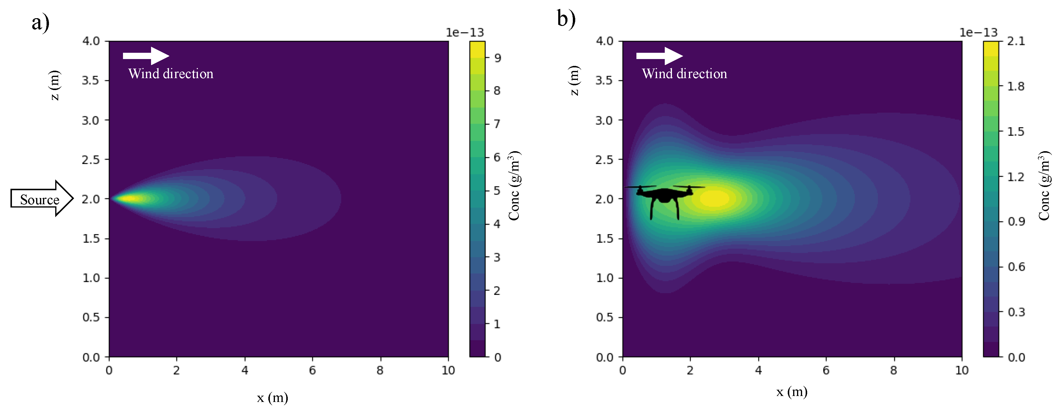
Figure 1a represents the distribution, in the absence of the drone, of the pollutant. It was obtained with the following: An emission mass flow rate of 1 g/s, a height of 2 m, conditions of neutral atmospheric stability, and a wind velocity of 1 m/s in a positive x direction. In the presence of a source of turbulence, the distribution of the pollutant is clearly affected. To determine the impact of the UAV passing close to the source of the pollutant, detailed dynamic fluid investigations would be required. For example, the one-equation Spalart–Allmaras of the Reynolds-Averaged Navier–Stokes turbulence model is one of the models commonly used to compute the turbulent eddy viscosity (TEV) [19,20]. The model gives TEV as result of a transport equation for a viscosity-like variable depending on turbulence production, dissipation, and diffusion of source terms. High-fidelity computational aerodynamics of multi-rotor UAV have shown that the maximum TEV is experienced in the areas directly below the turbine blades [21]. In this area, a turbulent mass flow of area moves vertically downwards with a lateral distribution, which is slightly larger than the size of the vehicle. Therefore, we can consider that there is an additive effect on σy and σz with a Gaussian dependence on distance according to the equation:
where P is the position of the vehicle and d the lateral dimension (of the vehicle). The K parameter represents the amount of turbulence induced by the propellers. The value of K increases as the vertical distance of the drone from the source decreases. This function is to be added to the two turbulence functions σy and σz. Figure 1b represents the concentration distribution of the pollutant when the vehicle is close to the source (P = 1 m). As seen from the shape of the concentration distribution, the presence of the vehicle significantly modifies the concentration distribution with respect to the actual condition (Figure 1a). Besides appearing more dispersed with lower average concentrations (note the difference in range of the color bar between Figure 1a,b), the distribution shape makes it apparent that the source of the pollutant has moved a few meters farther along x-axis. It should be noted that in Figure 1b, due to the strong turbulence induced by the UAV, the concentration of the pollutant at source seems to be nullified. The optical effect of the figure should not be misleading. The concentration at the source in the presence of the UAV is not zero. Although extremely simplified, our simulations show that drone-mounted sensors do not facilitate the correct mapping of the pollutant source position because the approach of a UAV modifies the spatial distribution of the substance/s under investigation. Note in Figure 1b that the position of maximum concentration (on the x-axis) shifted between 2 and 3 m. Quantitative information is also changed. In fact, note, for example, how the maximum intensity in the scale in false colors (representing the concentration distribution of the pollutant) is lower with a UAV (see Figure 1b) than without (see Figure 1a).
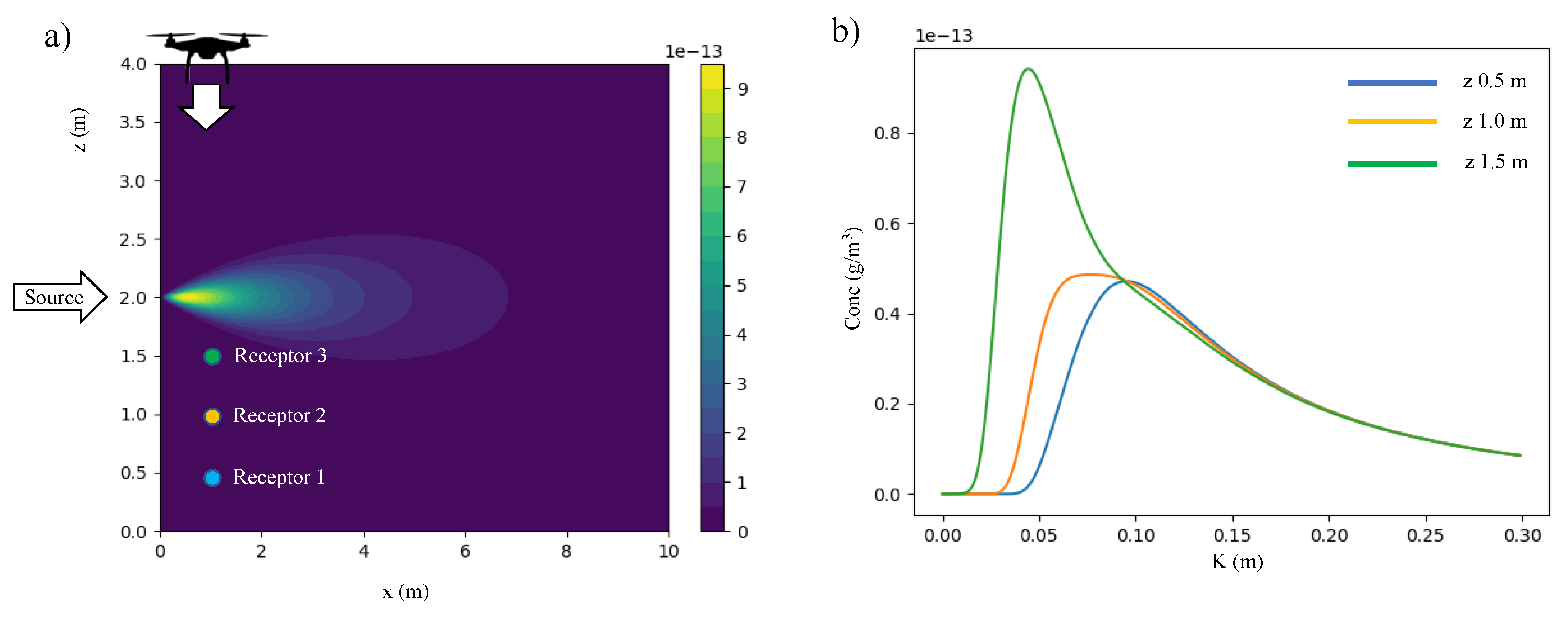
The physical meaning of K is related to the amount of turbulence induced by the drone below its airflow column. Indeed, it is related to the speed of rotation of the blades. Actually, the speed of rotation when in flight does not vary significantly; therefore, K can be considered to depend, in first approximation, mainly on the vertical distance between the vehicle and the point (placed below it) where the amount of turbulence is evaluated. If the drone is placed vertically at great distance from the receptor, K tends to zero. Conversely, K tends to be very high when close to the receptor. In fact, the closer it gets, the higher K tends to be. Figure 2 shows the effect of the increase of K, that is, of the drone proximity to the pollutant source, on the concentration of pollutant detected by three receptors placed at a distance of 1 m from the source along the x-axis and at heights of 0.5 m, 1 m, and 1.5 m on the z-axis, respectively. When the value of K is zero, that is, when the drone is far away from the source, the effect of the air vehicle is negligible and, under these simulated conditions, the concentration of the pollutant at the receptors is negligible. On the other hand, when K increases with the approach of the UAV, which fixes at its position x,y as it lowers along the z-axis towards the height at which the source is located, the pollutant is forcefully transported to the receptors. Indeed, Figure 2b shows an increase in the concentration detected by the receptors up to a maximum, above which the air is cleansed as the vehicle approaches. Although the turbulence induced by the drone is traced in an approximate way, our theoretical evaluations clearly indicate that with drone-mounted sensors the localization of pollutant source as well as its spatial distribution mapping is, to varying degrees, distorted and that this distortion depends on both the drone and receptor position.
3.2. In-Field Measurements
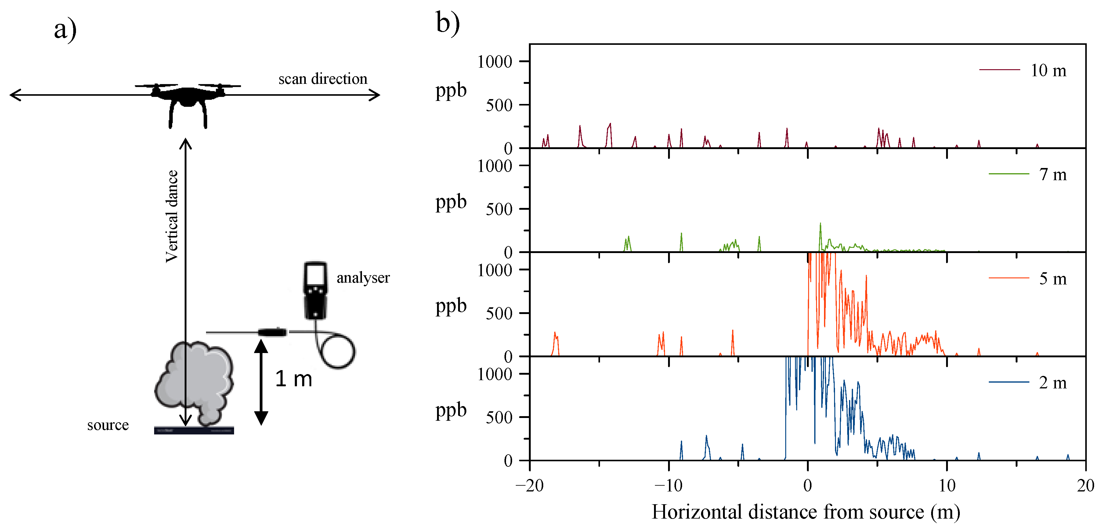
Given the results of the simulations, we decided to perform on-site analyses for the spatial distribution of pollutant concentration by means of UAV. Figure 3a schematically illustrates the experimental setup. A source of pollutant (a gasoline tank) was placed on the ground. A hydrocarbon analyzer was placed above it at a distance of 1 m, in which (in a quiet wind condition of <2 m/s) the concentration of hydrocarbons in the air is expected to be very low (<30 ppb). The pollutant concentration plots in Figure 3b were determined during UAV scans at variable heights.
Figure 3b shows that, when the drone flies at low heights (2 and 5 m), turbulent flows transport the pollutant toward the analyzer, thus significantly increasing the detected concentration. On the other hand, there is a height beyond which the effect of the drone passage is negligible. It was, therefore, necessary to implement an appropriate measuring system enabling the real-time, space-resolved detection of pollutants while avoiding turbulences induced by the drone. The approach proposed by us was to place the analyzer on the drone equipped with a long sampling probe that allows it to capture, by means of a pump, the volume of air to be analyzed from a zone that is not influenced by the drone (Figure 4a). Obviously, for a correct determination of the source position it is necessary to consider the delay in the determination of the substance due to the time required to travel through the sampling tube. However, knowing the flow rate of the suction pump and the size of the probe, it is possible to shift the detection time of the appropriate delay. By connecting the GPS position of the UAV, it was possible to reconstruct the mapping. Figure 4b,c reports the normalized concentration intensity false-color maps. Please note that the density of analysis points along the x-axis is much higher than along the z-axis. This is due to the fact that along the x-axis the density of points depends on the analysis capability of the sensor placed on the drone (one analysis every 10 s), while along the z-axis the pixel size depends on the distance between successive drone scans (about every 1.5 m).
The comparison between Figure 4b,c undoubtedly shows the effect of the vehicle on the precise position of the source. When the sampling probe was too short (2 m), the spatial distribution of the pollutant was completely distorted and, as expected, the turbulence induced by the vehicle caused a large dispersion of the pollutant (Figure 4b). For a correct determination of the spatial distribution, it was necessary to use a 10-m-long sampling probe (Figure 4c). Carrying out an extensive campaign of field experiments (not shown here for the sake of brevity), we were able to retrofit the simulations with the experimental data in order to find the suitable K values to be input into Equation (4) to obtain the minimum difference between the model prediction with what was detected by the sensor.
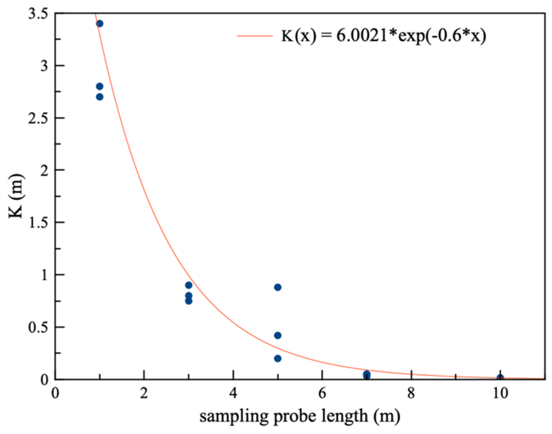
Figure 5 shows that there is an exponential relationship between the K parameter and the length of the sampling probe. Therefore, we derived an equation that allows us to evaluate the effect of UAV turbulence on the concentration of the pollutant, as follows:
where L is the length of the sampling probe and α is a parameter that depends on the type of vehicle used. It should be noted that in the calm wind conditions, in which the experiment was carried out, parameters I, J, and T can be considered constant and not influenced by environmental conditions. This equation may allow us to overcome the positional errors induced by turbulences when UAV flight height is not sufficiently high. However, its parameters markedly change with environmental conditions and they must be determined accordingly. Therefore, the employment of sufficiently long probes, preventing the generation of unwanted turbulent flows, is recommended.
4. Conclusions
In conclusion, we can confirm that, on the basis of theoretical forecasts and in-field experimental determinations, it is possible to perform correct mapping of pollutants by means of UAV, if they are equipped with sampling probes of appropriate length, overriding the effect of turbulence induced by helical engines. These results show, encouragingly, that this application is not only relevant and applicable to the precise leaks’ detection of discrete point source but also to various other contexts, including precision agriculture, for example, for determining the distribution of pollen and pheromones. The research, therefore, naturally moves on to the design of sensors capable of determining substances of interest.
Author Contributions
Conceptualization, N.T. and C.M.; methodology, N.T. and D.M.; data curation, N.T. and D.M.; writing—original draft preparation, N.T. and G.L.-D.; writing—review and editing; supervision, N.T. All authors have read and agreed to the published version of the manuscript.
Funding
The authors acknowledge “Piano della Ricerca” for APC.
Conflicts of Interest
The authors declare no conflict of interest.
References
- Everts, S.; Davenport, M. How drones help us study our climate, forecast weather. C&EN Glob. Enterp. 2016, 94, 34–36. [Google Scholar]
- Zhang, C.; Kovacs, J.M. The application of small unmanned aerial systems for precision agriculture: A review. Precis. Agric. 2012, 13, 693–712. [Google Scholar] [CrossRef]
- Diaz, J.A.; Pieri, D.; Wright, K.; Sorensen, P.; Kline-Shoder, R.; Arkin, C.R.; Fladeland, M.; Bland, G.; Buongiorno, M.F.; Ramirez, C.; et al. Unmanned aerial mass spectrometer systems for in-situ volcanic plume analysis. J. Am. Soc. Mass Spectrom. 2015, 26, 292–304. [Google Scholar] [CrossRef] [PubMed] [Green Version]
- Nathan, B.J.; Golston, L.M.; O’Brien, A.S.; Ross, K.; Harrison, W.A.; Tao, L.; Lary, D.J.; Johnson, D.R.; Covington, A.N.; Clark, N.N.; et al. Near-Field Characterization of Methane Emission Variability from a Compressor Station Using a Model Aircraft. Environ. Sci. Technol. 2015, 49, 7896–7903. [Google Scholar] [CrossRef] [PubMed]
- Bayat, B.; Crasta, N.; Crespi, A.; Pascoal, A.M.; Ijspeert, A. Environmental monitoring using autonomous vehicles: A survey of recent searching techniques. Curr. Opin. Biotechnol. 2017, 45, 76–84. [Google Scholar] [CrossRef] [PubMed] [Green Version]
- Aurell, J.; Mitchell, W.; Chirayath, V.; Jonsson, J.; Tabor, D.; Gullett, B. Field determination of multipollutant, open area combustion source emission factors with a hexacopter unmanned aerial vehicle. Atmos. Environ. 2017, 166, 433–440. [Google Scholar] [CrossRef] [PubMed]
- Gu, Q.; Michanowicz, D.R.; Jia, C. Developing a Modular Unmanned Aerial Vehicle (UAV) Platform for Air Pollution Profiling. Sensors 2018, 18, 4363. [Google Scholar] [CrossRef] [PubMed] [Green Version]
- Villa, T.F.; Salimi, F.; Morton, K.; Morawska, L.; Gonzalez, F. Development and validation of a UAV based system for air pollution measurements. Sensors 2016, 16, 2202. [Google Scholar] [CrossRef] [PubMed] [Green Version]
- Zhou, F.; Pan, S.; Chen, W.; Ni, X.; An, B. Monitoring of compliance with fuel sulfur content regulations through unmanned aerial vehicle (UAV) measurements of ship emissions. Atmos. Meas. Tech. 2019, 12, 6113–6124. [Google Scholar] [CrossRef] [Green Version]
- Dinkelaker, N.; Oripova, A.; Berman, I.; Pantiukhin, I.; Zavialova, I.; Bulatov, V. Comparative Analysis of Air Pollution Measurements between Compact Mobile Sensors and Standardized Laboratory Methods. Int. J. Electr. Electron. Eng. Telecommun. 2019. [Google Scholar] [CrossRef]
- Rossi, M.; Brunelli, D.; Adami, A.; Lorenzelli, L.; Menna, F.; Remondino, F. Gas-Drone: Portable gas sensing system on UAVs for gas leakage localization. In IEEE SENSORS 2014 Proceedings; IEEE: Piscataway, NJ, USA, 2014; pp. 1431–1434. [Google Scholar]
- Shigaki, S.; Fikri, M.R. Design and experimental evaluation of an odor sensing method for a pocket-sized quadcopter. Sensors 2018, 18, 3720. [Google Scholar] [CrossRef] [PubMed] [Green Version]
- Islam, A.; Houston, A.L.; Shankar, A.; Detweiler, C. Design and evaluation of sensor housing for boundary layer profiling using multirotors. Sensors 2019, 19, 2481. [Google Scholar] [CrossRef] [PubMed] [Green Version]
- Directive 2008/1/EC. Off. J. Eur. Union 2008, L25, 51.
- Faragó, I.; Georgiev, K.; Havasi, Á. (Eds.) Advances in Air Pollution Modeling for Environmental Security; NATO Science Series; Springer: Berlin/Heidelberg, Germany, 2005; Volume 54. [Google Scholar]
- Monitto, R.; Tuccitto, N. Shadow ribbon: A detailed study of complex chemical plants with a simple integrated approach. RSC Adv. 2014, 4, 32237–32240. [Google Scholar] [CrossRef]
- Vitale, S.; Zappalà, G.; Tuccitto, N. Filling station short-range impact on the surrounding area: A novel methodology for environmental monitoring based on the shadows study. Environ. Technol. Innov. 2015, 4, 210–217. [Google Scholar] [CrossRef]
- Pasquill, F. The Estimation of The Dispersion of Windborne Material. Meteorol. Mag. 1961, 90. [Google Scholar] [CrossRef]
- Spalart, P. Strategies for turbulence modelling and simulations. Int. J. Heat Fluid Flow 2000, 21, 252–263. [Google Scholar] [CrossRef]
- Spalart, P.R.; Allmaras, S.R. One-equation turbulence model for aerodynamic flows. Rech. Aerosp. 1994. [Google Scholar] [CrossRef]
- Ventura Diaz, P.; Yoon, S. High-Fidelity Computational Aerodynamics of Multi-Rotor Unmanned Aerial Vehicles. In 2018 AIAA Aerospace Sciences Meeting; American Institute of Aeronautics and Astronautics: Reston, VA, USA, 2018. [Google Scholar]
Figure 1.
(a) False-color map of the distribution of pollutant emitted from a source placed at 2 m above ground (see arrow). (b) Same conditions but with the unmanned aerial vehicle (UAV) placed at the same height as the source but at 1-m distance along the x-axis. Contours are from the model (Equation (1)). Please note that the scales of (a) and (b) are different to facilitate the reader’s eye.

Figure 2.
(a) Schematic representation of the simulated scenery. (b) Calculated pollutant concentration detected at the receptors as a function of K parameter representing the amount of turbulence induced by the propellers.
Figure 2.
(a) Schematic representation of the simulated scenery. (b) Calculated pollutant concentration detected at the receptors as a function of K parameter representing the amount of turbulence induced by the propellers.

Figure 3.
(a) Schematic representation of the in-field experimental setup. The analyzer probe was located 1 m above the source. (b) Hydrocarbons’ concentration detected by the analyzer during the drone’s scans above the source at various distances.
Figure 3.
(a) Schematic representation of the in-field experimental setup. The analyzer probe was located 1 m above the source. (b) Hydrocarbons’ concentration detected by the analyzer during the drone’s scans above the source at various distances.

Figure 4.
(a) Schematic representation of the in-field experimental setup. (b) False-color map of normalized hydrocarbons’ concentration detected by using 2-m-long sampling probe. Source position is indicated by the yellow arrow. (c) Same experimental conditions but with 10-m-long sampling probe. (d) In-field operation pictures.

Figure 5.
K value as a function of the sampling probe length. The red line draws the exponential best fit.
Figure 5.
K value as a function of the sampling probe length. The red line draws the exponential best fit.

© 2020 by the authors. Licensee MDPI, Basel, Switzerland. This article is an open access article distributed under the terms and conditions of the Creative Commons Attribution (CC BY) license (http://creativecommons.org/licenses/by/4.0/).
Share and Cite
MDPI and ACS Style
Li-Destri, G.; Menta, D.; Menta, C.; Tuccitto, N. Effect of Unmanned Aerial Vehicles on the Spatial Distribution of Analytes from Point Source. Chemosensors 2020, 8, 77. https://0-doi-org.brum.beds.ac.uk/10.3390/chemosensors8030077
AMA Style
Li-Destri G, Menta D, Menta C, Tuccitto N. Effect of Unmanned Aerial Vehicles on the Spatial Distribution of Analytes from Point Source. Chemosensors. 2020; 8(3):77. https://0-doi-org.brum.beds.ac.uk/10.3390/chemosensors8030077
Chicago/Turabian StyleLi-Destri, Giovanni, Dario Menta, Carmelo Menta, and Nunzio Tuccitto. 2020. "Effect of Unmanned Aerial Vehicles on the Spatial Distribution of Analytes from Point Source" Chemosensors 8, no. 3: 77. https://0-doi-org.brum.beds.ac.uk/10.3390/chemosensors8030077
Note that from the first issue of 2016, this journal uses article numbers instead of page numbers. See further details here.