
Skill and Inter-Model Comparison of Regional and Global Climate Models in Simulating Wind Speed over South Asian Domain


Department of Civil Engineering, Indian Institute of Technology Bombay, Mumbai 400076, Maharashtra, India
*
Author to whom correspondence should be addressed.
Climate 2022, 10(6), 85; https://0-doi-org.brum.beds.ac.uk/10.3390/cli10060085
Submission received: 15 May 2022
/
Revised: 10 June 2022
/
Accepted: 11 June 2022
/
Published: 16 June 2022
(This article belongs to the Section Climate Dynamics and Modelling)
Abstract
:Global Climate Models (GCMs) and Regional Climate Models (RCMs) have been widely used in understanding the impact of climate change on wind-driven processes without explicit evaluation of their skill. This study is oriented towards assessing the skill of 28 GCMs and 16 RCMs, and more importantly to assess the ability of RCMs relative to parent GCMs in simulating near-surface wind speed (WS) in diverse climate variable scales (daily, monthly, seasonal and annual) over the ocean and land region of the South Asian (SA) domain (11° S–30° N and 26° E–107° E). Our results reveal that the climate models’ competence varies among climate variable scales and regions. However, after rigorous examination of all climate models’ skill, it is recommended to use the mean ensemble of MPI-ESM-MR, CSIRO-Mk3.6.0 and GFDL-ESM2G GCMs for understanding future changes in wave climate, coastal sediment transport and offshore wind energy potential, and REMO2009 RCM driven by MPI-M-MPI-ESM-LR for future onshore wind energy potential assessment and air pollution modelling. All parent GCMs outperform the RCMs (except CCCma-CanESM2(RCA4)) over the ocean. In contrast, most RCMs show significant added value over the land region of the SA domain. Further, it is strongly discouraged to use the RCM WS simulations in modelling wind-driven processes based on their parent GCM’s skill over the ocean.
1. Introduction
Global warming has a direct impact on atmosphere circulation, where the wind is one of the important atmospheric variables. Changes in the magnitude and pattern of wind have a significant effect on evapotranspiration [1], air pollution modelling [2,3], wind energy [4,5], design of tall structures, wind-generated ocean waves [6,7,8], wave energy extraction [9], understanding coastal sediment transport [10,11] and ocean mixing [12]. The wind-driven processes, like wind-wave modelling, are very sensitive to the accuracy of the input wind climate [13]. Further, Macias et al. [14] identified wind speed as an important variable to correct bias in the sea surface temperature. Indeed, using the accurate wind speed not only improves the understanding of its variability due to climate change but also improves the wind-driven model simulations and wind-dependent climate variables.
Numerical climate models are primary and robust tools for understanding how the Earth’s climate system as a whole is likely to respond to future changes in energetics. The Global Climate Models (GCMs) collated under the World Climate Research Program’s (WCRP) Coupled Model Intercomparison Projects (CMIP3, CMIP5 and CMIP6) have been widely used in climate change impact studies [8,15,16,17,18,19]. Although GCMs have shown good skill in capturing climate variability at global scales, they fail to address the same at a regional or local scale; which is partially attributed to their coarser resolution [20,21]. Since climate change is having a significant impact on both global and regional scale processes [22], downscaling approaches, such as statistical [23,24,25] and dynamical downscaling [8,26,27], have been widely employed to overcome the shortcomings of GCMs and create region-specific climate data. WCRP’s Coordinated Regional Downscaling Experiment (CORDEX) started with a focus on providing the regional climate simulations for various adaptation and impact assessment studies using Regional Climate Models (RCMs). RCM outputs are also widely used in climate applications, like understanding extreme precipitation events over southern Africa [28,29], precipitation patterns of summer monsoon over India [30], precipitation and temperature over West Africa [31], meteorological drought at a global scale [32], capturing the circulation pattern of Etesian over eastern Mediterranean [33], extreme winds over Germany [34] and Europe [35] and reproducing features of tropical cyclones around Japan [36]. It is expected that RCMs should accurately represent the regional processes because of their finer resolution and region-specific parameterization. However, it is found that RCMs are underestimating the intense wind speeds over Europe [34,35], and overestimating the wind speed over the Arabian Sea (AS) and Bay of Bengal (BoB) [37]. Winterfeldt and Weisse [38] found that RCMs show good skill in representing wind speed over coastal areas and poor skill over the open ocean. This indicates RCMs’ skill is region-specific and they do have a systematic bias inherited from the parent GCM and self-induced bias. In the South Asian (SA) region, the skill of all available CORDEX RCMs in representing the near-surface wind speed (WS) is not addressed yet. Notable studies [39,40,41,42,43] have investigated the skill of GCMs over the ocean part of the SA domain, but the skill of GCMs over the land part of the SA domain needs to be investigated further. Moreover, the added value of RCMs relative to their corresponding parent GCMs in representing WS over the SA domain is still unknown. Torma et al. [44] found the added value of using high-resolution RCMs than the corresponding driving GCMs in representing precipitation over complex topographic features of the Alpine region. On the contrary, Singh et al. [45] found no consistent added value by RCMs relative to corresponding parent GCMs in representing Indian summer monsoon rainfall characteristics. Kulkarni et al. [46] evaluated three RCMs and their parent GCMs in simulating the offshore WS along the Indian coast and found no significant added value by RCMs. This highlights that the added value of RCMs is regional and variable-specific and needs to be evaluated before using them in regional climate impact studies.
A brief review on indicators (mostly used are Skill Score, Taylor diagram, correlation coefficient, root mean square error and absolute error) used in the selection of GCMs to represent precipitation, temperature (mean, maximum and minimum) and monsoon (East Asian, Indian summer, Australian, West African summer) characteristics over different regions of the world are well presented by Raju and Kumar [47]. They observed that most studies failed to report the basis of selecting a particular indicator, simple methodology to collate the different unit metrics to a single score to rank GCMs and technique to select the subset of GCMs as part of the ensemble. Further studies showed that the constructed best-performing GCM is sensitive to the chosen decision technique, the number of indicators considered and the variable of interest [48,49]. Mohan and Bhaskaran [40] evaluated the skill of 35 CMIP5 GCMs using the Taylor skill score and recommended the model constructed from the mean ensemble of the top ten GCMs in representing monthly mean WS qualitatively, but no quantitative logic behind the selection of the ten GCMs is presented. Furthermore, while the identified top GCMs did a good job of portraying the monthly mean WS, we cannot assume the same level of performance when it comes to representing diverse climatic variable scales (daily, seasonal and annual). As a result, to rank climate models, a composite metric (including all climatic variable scales) with suitable assessment statistics and weights is required. Even though Kulkarni et al. [46] assessed the performance of only three RCMs and GCMs, the study region was restricted to the offshore region along the Indian coast. A recent study by Morim et al. [50] shows that inter-model uncertainty is two to four times greater than the uncertainty associated with model internal variability. This emphasizes the need for evaluating a greater number of climate models over diverse climate variable scales to reduce the model-based uncertainty.
With the backdrop of the above discussion, this study aims at evaluating the skill of all available individual CMIP5 GCMs and CORDEX RCMs in representing near-surface wind speed (WS) on diverse climate variable scales (daily, monthly, seasonal and annual scales) over the ocean and land parts of the South Asian (SA) domain. Furthermore, we investigated the added/detriment of RCMs’ skill in simulating WS over the ocean and land of the SA domain relative to the corresponding parent GCMs. Since a comprehensive evaluation method is still absent to assess and construct the best suitable model/ensemble of models in reproducing the annual, seasonal, monthly and daily mean WS climate, a new approach called Relative Score is devised and presented.
2. Materials and Methods
2.1. Climate Models and Reference Data
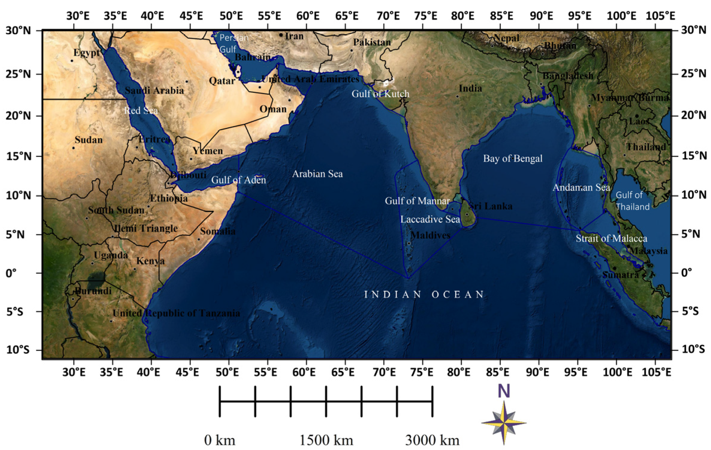
This study evaluated the performance of climate models (sixteen CORDEX RCMs and twenty-eight CMIP5 GCMs, listed in Table 1 and Table 2) in simulating the near-surface wind speed (WS) over the South Asian (SA) domain (11° S to 30° N and 26° E to 107° E, refer to Figure 1). The extent of the SA domain is bound by the joint availability of wind data from all CORDEX RCMs. Based on the availability of wind field data from climate models and the Fifth Generation European Research Agency (ERA5), a common time slice of 27 years from 1979 to 2005 and a present time slice of 14 years from 2006 to 2019 were considered to assess climate models. Even though the present time slice of WS projections was available from four different RCP scenarios (RCP2.6, RCP 4.5, RCP6 and RCP8.5), due to similar radiative forcing not much difference in the skill of climate models was expected for all four scenarios [40]. As a result, the moderate RCP scenario (RCP 4.5) was considered. The daily mean WS zonal and meridional components were downloaded from the Earth System Grid Federation portal (https://esg-dn1.nsc.liu.se/search/cordex/, accessed on 1 January 2020 and https://esgf-node.llnl.gov/search/cmip5/, accessed on 11 January 2021). To examine inter-model variability, we analyzed climate model WS data from one realization, initial conditions and model physics (r1i1p1) ensemble.
Diverse reference datasets were available and used in understanding wind climate studies: satellite data [40], ERA-Interim [51,52,53,54,55], ERA-40 [56], Climate Forecast System Reanalysis (CFSR) [46] and ERA5 [50,57,58,59,60,61]. Kulkarni et al. [46] evaluated the CFSR, ERA-Interim and NCEP WS reanalysis data over the Indian offshore region and recommended ERA-Interim among the three reanalysis datasets. Krishnan and Bhaskaran [41] found that ERA-Interim is better than CFSR in representing wind climate over BoB. In general, the availability of long-term reliable and precise data with a higher spatial and temporal resolution will influence the usage of reference data to evaluate climate model performance. In-situ observations and measurements from buoys are limited to specific locations, whereas satellite-based measurements are not limited in space but are not available over a long period of time. Due to these constraints, the performance of climate models was evaluated with reference to reanalysis data in lieu of observational data. A recent study by Molina et al. [62] found a significant correlation (0.9–0.95) between ERA5 daily WS and HadISD stations data, and concluded that the ERA5 can be used for validation of a climate model simulation. Morim et al. [50] considered the atmospheric reanalyses as powerful tools for modelling and analysis of climate models over spatio-temporal scales, and used the ERA-Interim and ERA5 for the inter-comparison of AGCM, AOGCM and ESM in simulating the surface wind fields globally. Further, for the development of offshore wind farms [60,63,64] and investigation of the climate change impact on offshore wind energy [59], the ERA5 dataset is used. Over the IO region of the SA domain, Naseef and Kumar (2020) [58] studied the wind and wind-generated wave climatology using an ERA5 dataset. Hence, the latest ERA5 wind data was used as a reference dataset, which is an improved version of its predecessor ERA-Interim [65,66,67]. The reference wind datasets (ERA5) were downloaded from Copernicus Climate Change Service Climate Date Store (https://cds.climate.copernicus.eu/, accessed on 1 January 2020) at an hourly scale, having a spatial resolution of 0.25° × 0.25°.
2.2. Methodology
A most popular method [68], and the best in bias reduction among other bias correction techniques [69], named quantile mapping developed by Li et al. [70] was used for bias correction. The climate variables (u and v components of near-surface wind speed) from all the climate models are available at different horizontal grid resolutions (0.44 × 0.44 for CORDEX RCMs, and for CMIP5 GCMs refer to Table 1). To remove the bias using the quantile mapping technique and to evaluate the models’ skill, all the models and reference datasets should be at the same spatial resolution. Hence, each model output was interpolated to a common horizontal grid resolution of 0.25° × 0.25° by using the Climate Data Operator remapbil function [71]. For a detailed description of the bilinear interpolation method used in the remapbil function, refer to the user guide of the Spherical Coordinate Remapping and Interpolation Package (SCRIP) [72]. Although the reference data for the present time slice (2006–2019) are available, we treated it as a future time slice and bias-corrected to examine the accuracy of bias-corrected present time slice climate model projections. The normal distribution was fitted to the daily time series of both zonal and meridional components of WS as it proved to be the best fit, and further correcting WS components will automatically correct the wind direction. Note that, hereafter, the WS dataset of climate models is, by default, the bias-corrected dataset.
A devised Relative Score (RS) approach was used to evaluate the performance of climate models on a daily, monthly, seasonal and annual scale. The RS was calculated using Equation (1) for each assessment criteria statistic, and it ranged from 0 to 1. RS will be 1 if the climate model perfectly simulates the observed conditions, and it will be 0 if the model is poorly simulated. Table 3 lists the Assessment Criteria Statistics (ACS) and weighting factors used to assess the skill of models, which will be detailed in the following section. The final rank is assigned to each model based on the Total Relative Score (TRS), which is the summation of all individual assessment criterion RS in both the time slices.
where
= Relative Score of ith model for jth assessment criteria;
= jth assessment criteria statistic value between ith model and reference data;
= maximum assessment criteria statistic value for the jth assessment criteria statistic;
= minimum assessment criteria statistic value for the jth assessment criteria statistic;
= weighting factor;
= number of assessment criteria.

Table 3.
Summary of assessment criteria statistics used to evaluate models at various climatic variable scales.
Table 3.
Summary of assessment criteria statistics used to evaluate models at various climatic variable scales.
| Climate Variable Scale | Method/Statistic | Assessment Criteria Statistic (ACS) | W |
|---|---|---|---|
| Daily mean | Perkins Skill Score (PSS) | Bias in PSS ) | 0.5 |
| Spatio-temporal variability | Empirical Orthogonal Function (EOF) analysis
| Empirical Orthogonal Function (EOF) analysis
| 1 |
| Annual cycle | Statistical significance of positive ‘r’ | 1 | |
| Annual mean | Statistical significance of bias | Percentage of statistically significant bias | 0 |
| Seasonal mean | 1 | ||
| Annual mean trend | Mann–Kendall (MK) test Theil-Sen slope | Mean Absolute Bias of trend | 1 |
| Seasonal mean trend | 1 | ||
| W= weighting factor r = correlation coefficient | |||
| = percentage of statistically insignificant positive correlation coefficient | |||
The climate model’s ability to reproduce the frequency distribution of daily mean WS was assessed by comparing the climate model’s whole study domain probability distribution to the ERA5 dataset using the Perkins Skill Score (PSS) [73]. The PSS is a tool for calculating the area shared by two probability density functions. It has a range of 0 to 1, with 0 indicating no overlap and 1 indicating perfect overlap. For each climate model, the RS is calculated using the bias in PSS () as an ACS, which is defined as one minus PSS.
where n is the number of bins, is the bin width, is the frequency density value of the model in a given ith bin and is the frequency density value of reference data in a given ith bin.
An Empirical Orthogonal Analysis (EOA) was carried out to characterize the spatial and temporal variability of monthly mean WS over the study domain. In this study, the first mode of EOF (EOF1), which explains more fractions of total variance, and its corresponding principal component (PC1), which explains how this EOF1 pattern oscillates over time, were analyzed. EOF1 was obtained for each GCM and compared with ERA5. The ability of GCM in reproducing the dominant mode of monthly mean WS climate was evaluated by calculating the absolute bias in the percentage of variance explained by EOF1, and to assess GCM performance in representing the spatial oscillating pattern, the whole domain mean absolute bias () was calculated as per Equation (4). The correlation coefficient and mean absolute bias of PC1 () between GCM and ERA5 were used as assessment criteria statistics to calculate RS.
where is the total number of grid cells, and and are the EOF1 magnitude of model and reference data at ith grid, respectively.
where is the total number of months, and and are the PC1 magnitude of model and reference data of the ith month, respectively.
The ability of the climate model to reproduce the annual cycle pattern as observed by ERA5 was assessed using the correlation coefficient. The long-term monthly mean was determined by averaging the monthly WS across a 27-year period for the historical time slice and 14-year period for the present time slice (with a sample size of 12). The t-test at a significance threshold of 0.001 was used to calculate the statistically significant positive correlation between the climate model and ERA5. For each GCM, the percentage of statistically significant positive correlation () was calculated by taking the ratio of the number of significant grid points to the total number of grid points in the study domain. Finally, the percentage of statistically insignificant positive correlation coefficient () was used as ACS.
The annual and seasonal mean wind speeds were calculated for all climate models and ERA5 at every spatial grid location of the study region. In general, the model bias is defined as the modelled dataset minus the referenced dataset, that represents the deviation of the model dataset from the reference dataset. To evaluate the statistical significance of this bias, a t-test was used with a significance level of 0.001. The percentage of statistically significant bias ( ratio of the number of significant bias grid points to the total number of grid points) is computed and used as ACS to calculate RS.
The models’ ability to capture the observed trend was tested. The Mann–Kendall (MK) non-parametric rank-based test [74,75] was used to identify the monotonic trend and the Theil-Sen slope [76] was used to estimate the magnitude of the trend in annual mean and seasonal mean WS. Wang et al. [77] recommended to increase the significance level and sample size/time series to improve the power of the MK test. As a result, in this study the significance level of 0.1 was used. The whole domain mean absolute bias () in trend magnitude was estimated using Equation (6) and used to calculate RS.
where is the total number of grid cells, and and are the model and reference trend magnitude at ith grid, respectively.
3. Results and Discussion
The literature [40,78,79,80,81] suggests that an ensemble of multiple climate models performs better compared to individual models. As a result, the skills of the mean ensemble of all climate models, as well as the top-performing climate models, were evaluated. Due to the complex topography over continents, the performance of climate models over the ocean and land may differ, so the skill of climate models in reproducing the WS over ocean and land was assessed separately in this study.
3.1. Skill of Climate Models in Reproducing WS Climate over Diverse Climate Variable Scales
3.1.1. Daily Mean Wind Speed
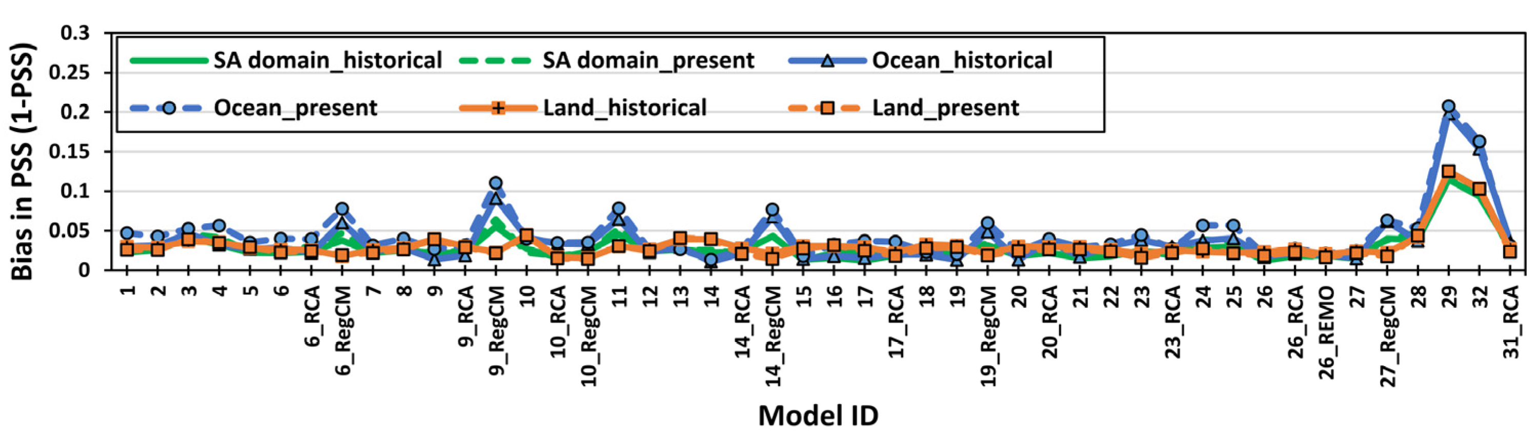
The entire SA domain frequency distribution of daily mean WS was captured well by all the individual GCMs and RCMs with a minimum PSS of 0.9545 and 0.9449, respectively. Over both regions of the SA domain, a similar PSS was observed in both time slices. In the case of RCMs driven by the same GCMs, RegCM type RCMs had a higher ACS (i.e., lower skill) compared to RCA type RCMs over the SA domain ocean (Figure 2). The frequency distribution differed greatly (resulted in higher PSS) for MMEs (models 29 and 32) due to averaging while determining the ensemble mean WS from the corresponding models. Table S1 tabulates the computed RS (sum of RS acquired for each time slice) of each climate model over the SA ocean and land.
3.1.2. Spatio-Temporal Variability of Monthly Mean Wind Speed
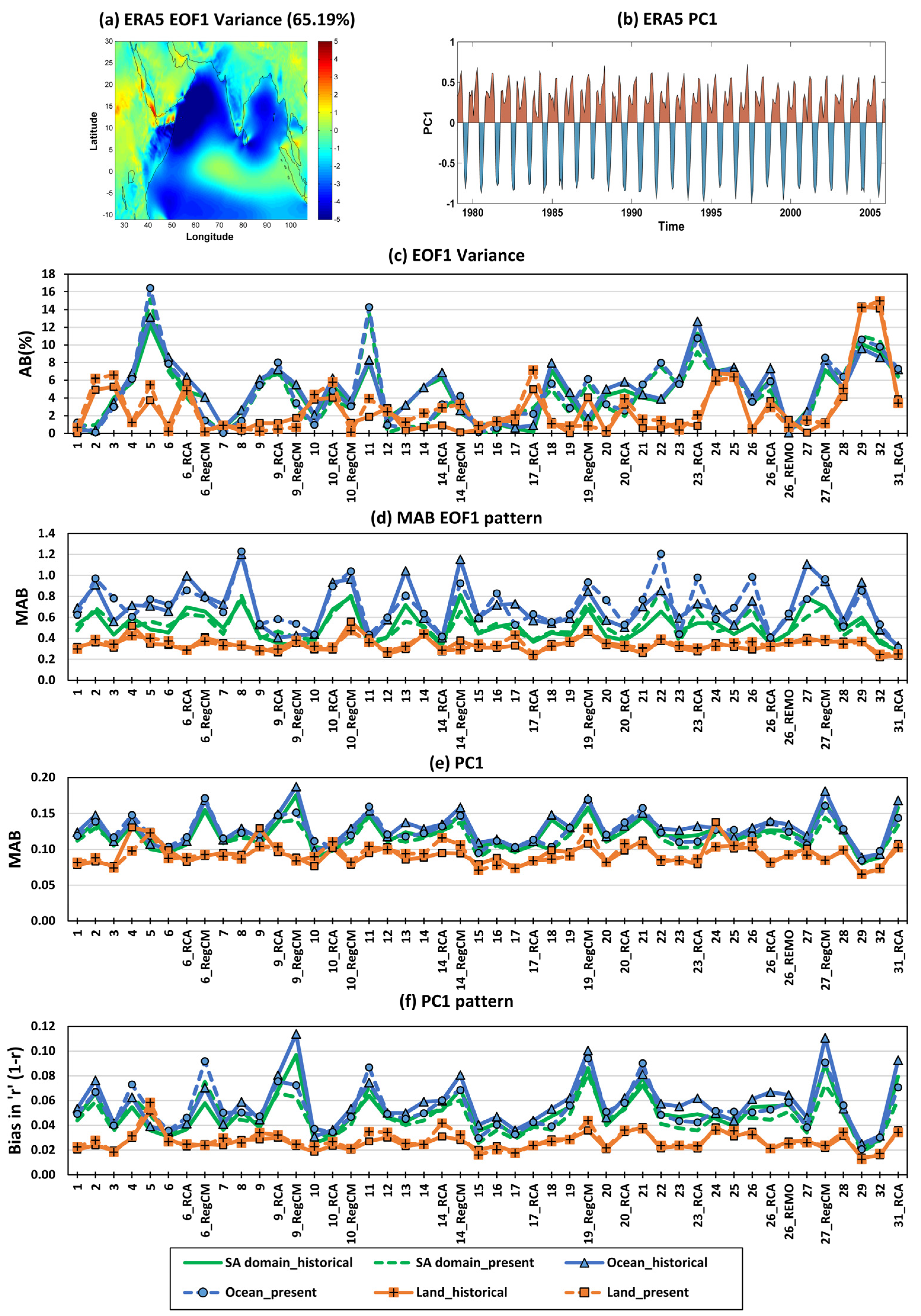
The ability of GCMs and RCMs in reproducing the magnitude and pattern of EOF1 and PC1 is discussed in this section. The ACS summary of each GCM and RCM is shown in Figure 3c–f, and estimated RS is tabulated in Table S2. The climate models’ ACS was almost same in both time slices, and it was lesser over SA land compared to the ocean. The ERA5 historical monthly mean WS EOF1 accounted for 67.71%, 56.14% and 65.19% of the total variance over the ocean, land and entire SA domain, respectively. The maximum WS variability was observed along the flow of Somali Jet (Figure 3a). Most of the climate models had AB below 8% in representing the percentage of variation, whereas model 5 had a maximum of 16.43% AB over SA ocean in the present time slice. Overall, the GCMs 15 and 17 (26_REMO) showed higher skill in capturing the spatio-temporal variability of monthly mean WS over the SA ocean and SA land relative to all individual GCMs (RCMs) (Table S2). All the parent GCMs outperformed RCMs over the ocean region of the SA domain, whereas over the land region of the SA domain, RCMs (excluding RCMs driven by 14, 19 and 20) showed higher skill relative to parent GCM. When the MMEs of CMIP5 and CORDEX were compared over the SA domain, the MME_CMIP5 skill was found to be greater (11.66 % over ocean and 5.83 % over land) than MME_CORDEX (Table S2). Even though MMEs showed poor skill in estimating the EOF1 variance (AB > 8.5% over ocean and AB > 14% over land), both MMEs showed greater skill in reproducing the EOF1 pattern, PC1 pattern and PC1 magnitude compared to most individual climate models (Figure 3c–f). All climate models showed higher skill over land relative to ocean because of less variability of the monthly mean WS over land.
3.1.3. Annual Cycle
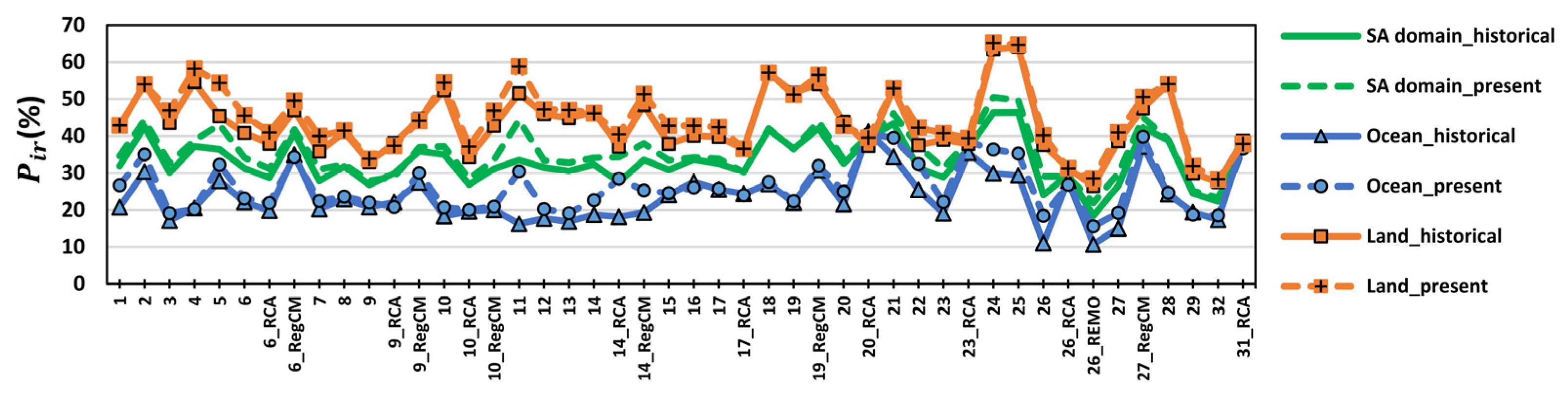
The computed entire domain mean correlation coefficient ranged from 0.68 to 0.9 over the SA domain. All the climate models showed higher over the land compared to ocean in capturing annual cycle variation over the SA domain (Figure 4). The was the same in both study time slices for most climate models over the SA domain. The climate models were sorted in descending order of their skill, based on computed RS, tabulated in Table S3. Over the SA ocean, models 26_REMO (MPI-M-MPI-ESM-LR(REMO2009)), 26 (MPI-ESM-LR) and 27 (MPI-ESM-MR) performed well in both time slices with least . The 26_REMO not only performed well over the ocean but was also the top-performing model over land. Over the SA land, the ensemble of twenty-eight GCMs (MME_CMIP5) had a higher skill in capturing annual cycle variation relative to all individual GCMs. The MMEs showed similar skill in capturing annual cycle patter; however, MME_CORDEX had a slightly higher (4.62% over ocean and 8.68% over land) RS compared to MME_CMIP5 (Figure 4 and Table S3). Models 24 and 25 showed lower skill over both ocean and land. The 27_RegCM showed poor skill in capturing the annual cycle pattern over the SA domain, even though its parent GCM MPI-ESM-MR showed moderate skill. Parent GCMs performed better in capturing annual cycle variation than RegCM type RCMs, except for model 10. This inference agrees with Herrmann et al. [82], who observed that parent GCMs show a higher correlation than RCMs in capturing annual cycle variation over South East Asia.
3.1.4. Seasonal Mean Wind Speed
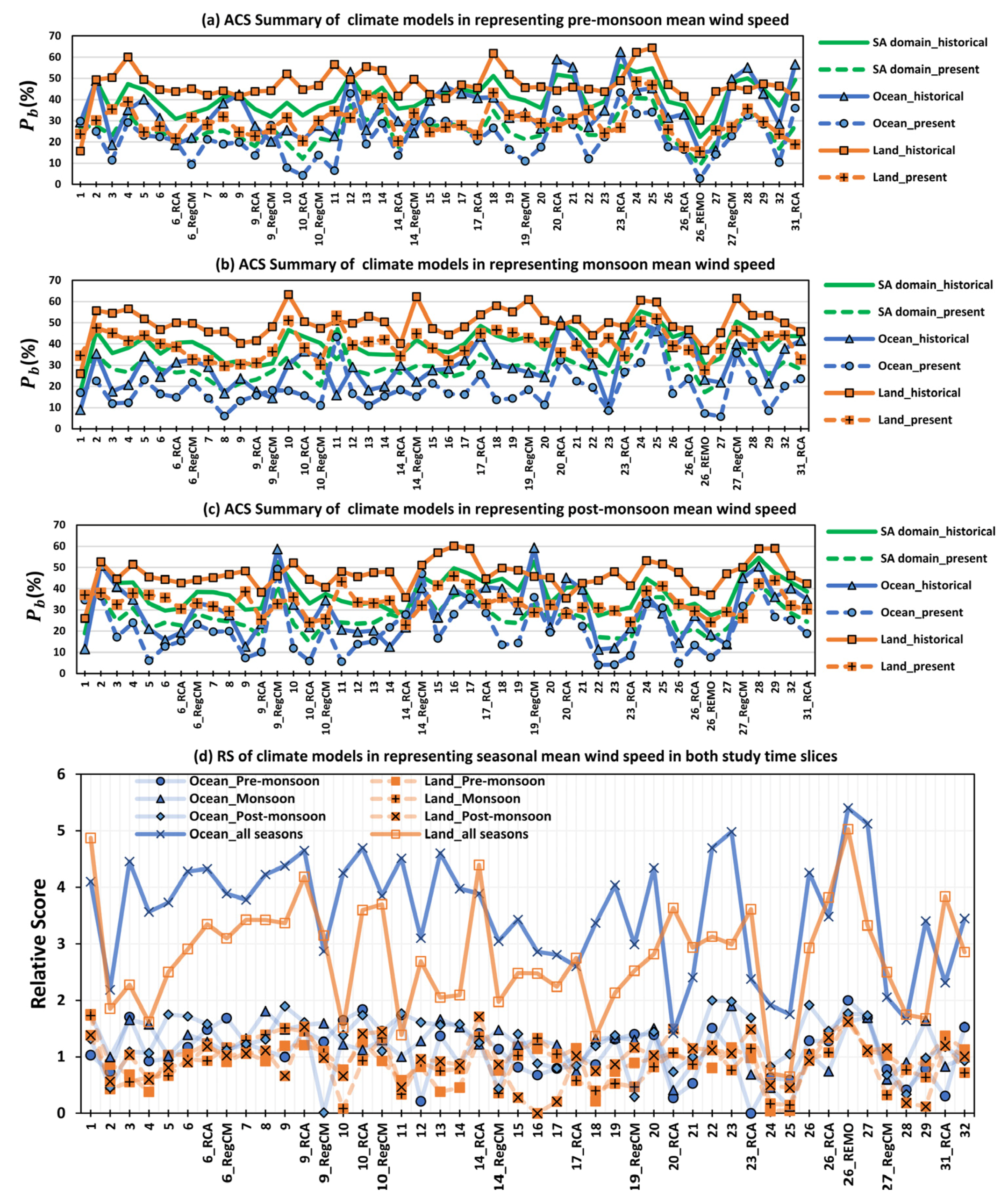
The current study domain has a distinct weather system with three different monsoons. In all seasons, the mean WS was strengthening along the coastal region of Kenya and Somalia, the western part of Sumatra, and weakening over the northwestern BoB along the Indian coast (Figure S1). The ERA5 accurately captured the most well-known tropical low-level jet known as the Somali Jet (Figure S1), which plays a major role in wave climate over AS [83]. In all seasons, a higher percentage of statistically significant bias () was observed over land compared to the ocean region of the SA domain, and was higher in the historical time slice (Figure 5a–c). Over the SA ocean, the pre-monsoon (February–May) mean WS climate was well-captured by 26_REMO, 10_RCA, 11, 3, 27,6_RegCM and 10 climate models. Only 26_REMO performed well over the ocean and land regions of the SA domain in all seasons. Among CMIP5 GCMs, after ACCESS1.0 (model 1), the MPI-ESM-MR (model 27) showed a higher skill in capturing seasonal mean WS (Figure 5d). MPI-ESM-LR (model 26) and MPI-ESM-MR have similar model dynamic components, whereas the former had a higher skill because of its higher spatial resolution. Müller et al. [84] found a reduction in biases of upper-level zonal wind and atmospheric jet stream position in the northern extratropics by MPI-ESM1.2-HR, which is a successor to MPI-ESM1.2-LR with a higher spatial resolution (~twice). A recent study by Desmet and Ngo-Duc [85] found MPI-ESM1.2-HR as the best CMIP6 GCM in representing seasonal 850-hPa wind over South East Asia for the historical period 1985–2014. Thus, findings from this study may help the research community to directly choose the climate model with similar model dynamic components from CMIP6 GCMs. Models 24 and 25 consistently showed poor skill with higher over the SA domain in all seasons (Figure 5). These models are not recommended in inter-seasonal variation studies.
Model 1, which performed well over the SA land has shown moderate skill over the SA ocean in all seasons. Further, model 23 performed well over the SA ocean, but it showed moderate performance over SA land in all seasons. Models 9_RegCM and 19_RegCM showed good skill in pre-monsoon and monsoon relative to post-monsoon over the SA ocean (Figure 5d). Thus, the model that performs well in one particular season or region does not necessarily perform well in another season or region. This emphasizes the importance of assessing the climate model skill over different seasons and regions (land and ocean).
The MME_CMIP5 (model 29) and MME_CORDEX (model 32) had similar skills over the SA ocean in all seasons, except in monsoon season. Over the SA land, the MME_CORDEX showed higher skill than MME_CMIP5 in representing all seasonal mean WS. However, both MMEs showed moderate skill relative to the top-performing climate model (Figure 5d). Thus, the ensemble of all climate models need not be considered as a reliable one. In the top ten performing climate models over land, most of them were RCMs rather than GCMs; however, over the ocean, most of GCMs were in the top-performing climate models compared to RCMs (Table S4). Thus, RCMs’ WS projections can be used over land in inter-seasonal studies, rather than GCMs.
3.1.5. Seasonal Mean Wind Speed Trend
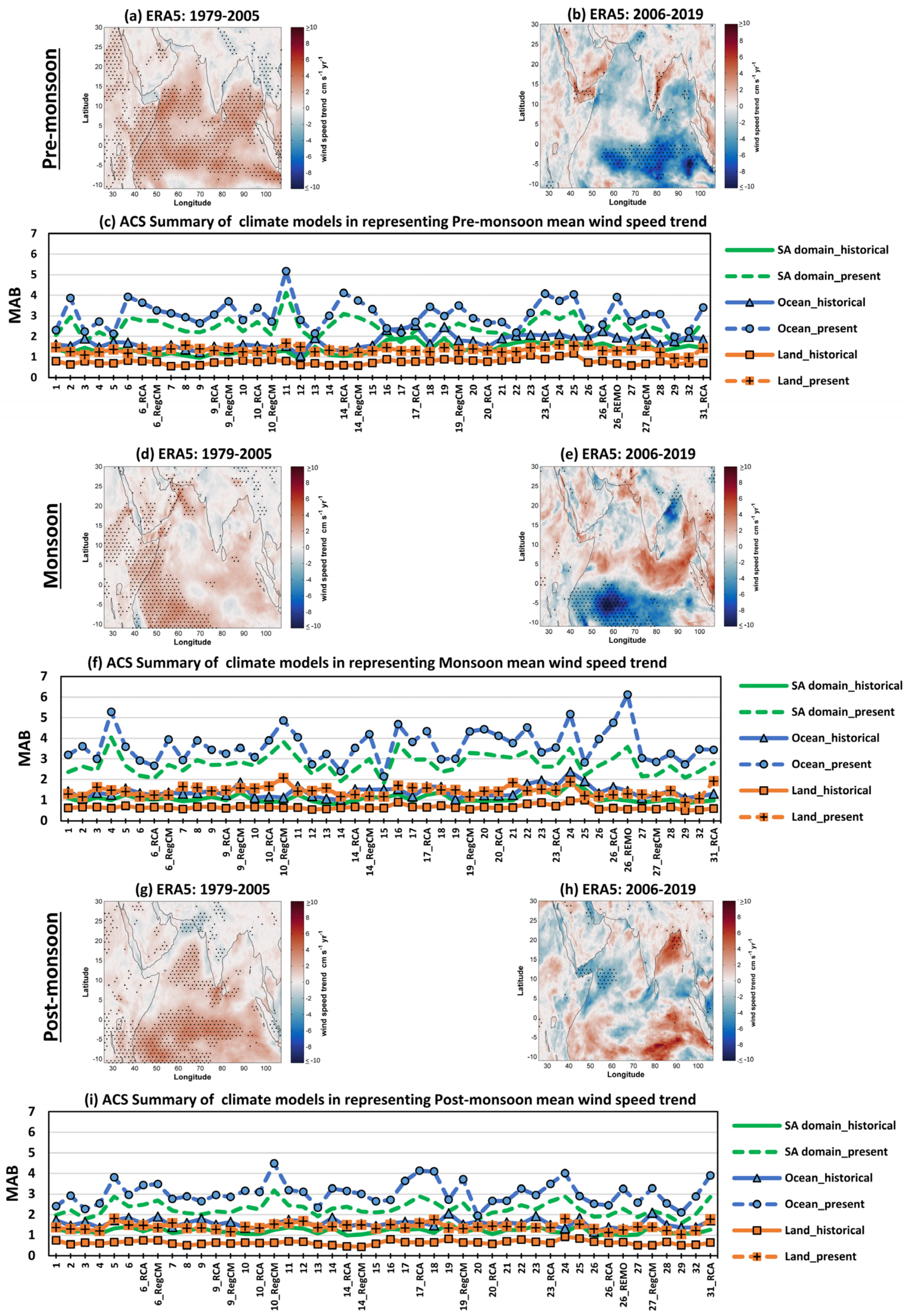
The skill of the climate models to capture the seasonal mean WS trend was assessed by calculating the mean absolute bias of trend magnitude. The statistically significant increasing trend was observed along this Somali Jet as shown in Figure 6d. However, in the present time slice, the decreasing monsoon WS trend was observed along most regions of the Somali Jet and was higher over the south of the equatorial region, most of AS and BoB (Figure 6e), which indicates the weakening of the south-west monsoon. In all seasons, the MAB of the climate model in capturing the seasonal mean WS trend was higher over the SA ocean than on land, and less variance in MAB was observed over SA land (Figure 6c,f,i). This is because the WS trend varied less across the land. Tables S5–S7 show the computed RS of each climate model for each season. Model 26_REMO consistently showed better skill in capturing the seasonal mean WS (Figure 5), whereas it failed to capture the seasonal mean WS trend over both ocean and land in all seasons (Figure 6). The seasonal mean WS trend was reliably captured by none of the individual climate models over the SA domain. Tian et al. [86] evaluated the skill of all CMIP5 GCMs considered in this study (except models 5 and 9) in reproducing the WS trend relative to observation data from the Integrated Surface Database, initiated by the National Centers for Environmental Information for 1979–2005 over the Northern Hemisphere. They found CMIP5 GCMs show poor skill in simulating the long-term temporal trends of surface winds. However, the ensemble of all GCMs (MME_CMIP5; model 29) has consistently performed well in capturing the seasonal mean WS trend over ocean and land (Figure 6). On the other hand, MME_CMIP5 failed to capture the seasonal mean WS over both ocean and land (Figure 5). Thus, climate models’ ability to capture the seasonal mean WS and its trend vary. This emphasizes the need of assessing whether a climate model can reproduce a climatic variable’s mean and trend. MME_CORDEX also showed a skill similar to MME_CMIP5 over land, but it showed moderate skill in capturing the seasonal mean WS trend over the ocean (Table S8). We can ascribe the benefit/detriment of the MMEs to the compensation of individual climate model biases during a mean arithmetic operation. However, selecting the appropriate climate models as part of the ensemble member is critical. Model 24 showed very poor skill in capturing seasonal mean WS trend, followed by 25 and 11.
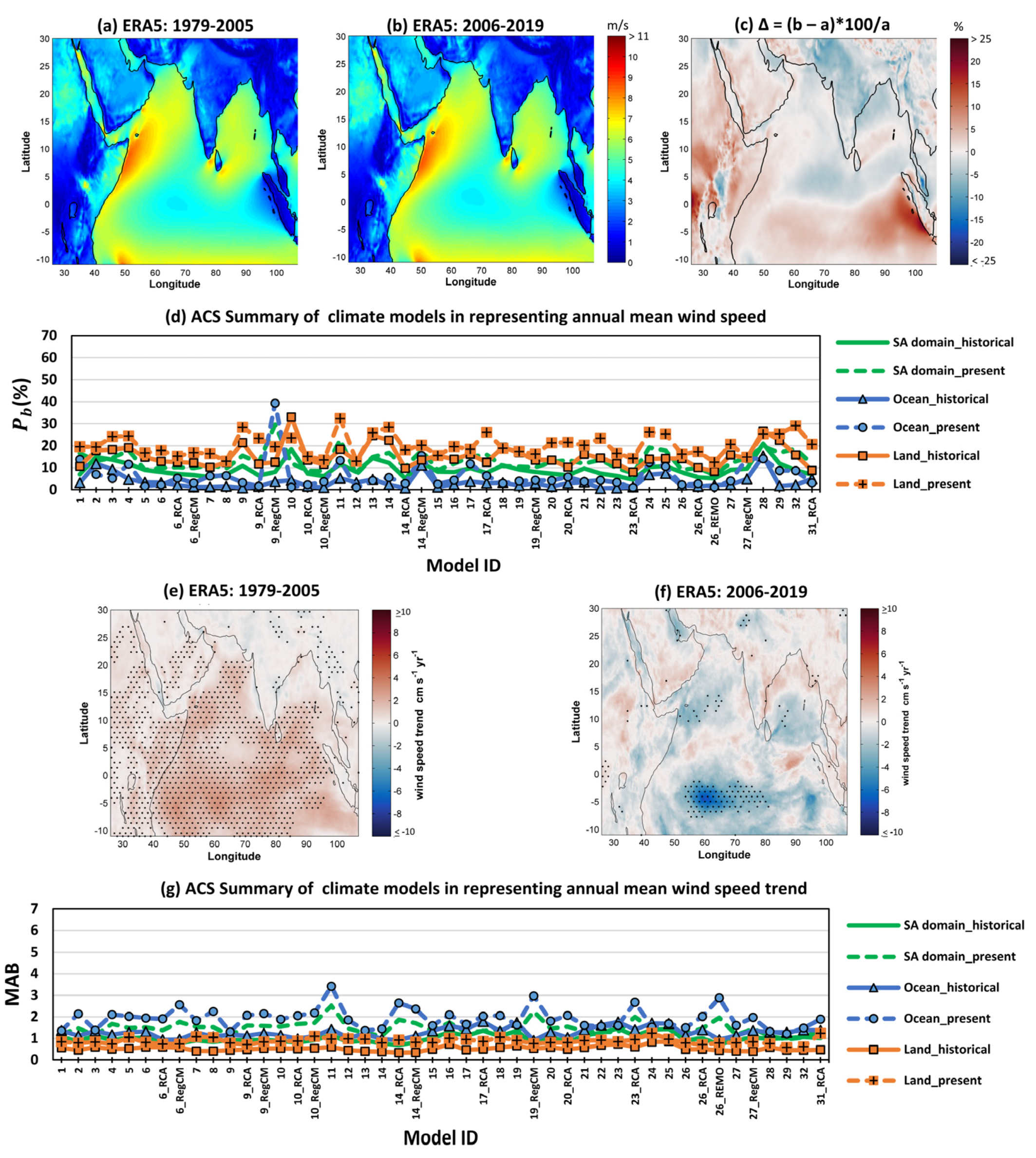
3.1.6. Annual Mean Wind Speed and Its Trend
Over the ocean, most of the climate models showed less (close to zero) in representing annual mean WS climate (Figure 7) and more (on average 8.7 times in the historical period) in representing seasonal mean WS (Figure 5). The 27-years annual mean WS was the same as the mean of all daily WS due to bias correction with the quantile mapping technique. This technique ensured that all the statistical properties of the model matched well with reference data over the considered time slice. However, the statistical properties of models and the reference dataset might not match well over the intermediate time slice, which led to higher bias over the seasonal scale. As a result, the climate models’ skill was evaluated as a seasonal scale considering the weighting factor as one, and zero for the annual mean WS climate assessment. Increasing annual mean WS was observed over most parts of the SA ocean in the historical time slice, whereas the decreasing trend was observed in the present time slice (Figure 7e,f). The decreasing trend of 1–2 cm/s/yr was observed along the central east and west coast of India, and the same was reported by Shanas and Kumar [87]. Most of the models showed a similar skill in reproducing the observed annual mean WS trend, whereas model 11 showed poor skill with higher MAB over the SA ocean (Figure 7g). A statistically significant increasing trend was observed over most parts of the SA ocean in the historical time slice, whilst the significant decreasing trend was observed in the present time slice in all seasonal and annual scales (Figure 6 and Figure 7). All of the models failed to reflect this shift in trend pattern and magnitude, resulting in a larger MAB in the present time slice. The estimated RS of each climate model in capturing the annual mean WS trend is tabulated in Table S9.
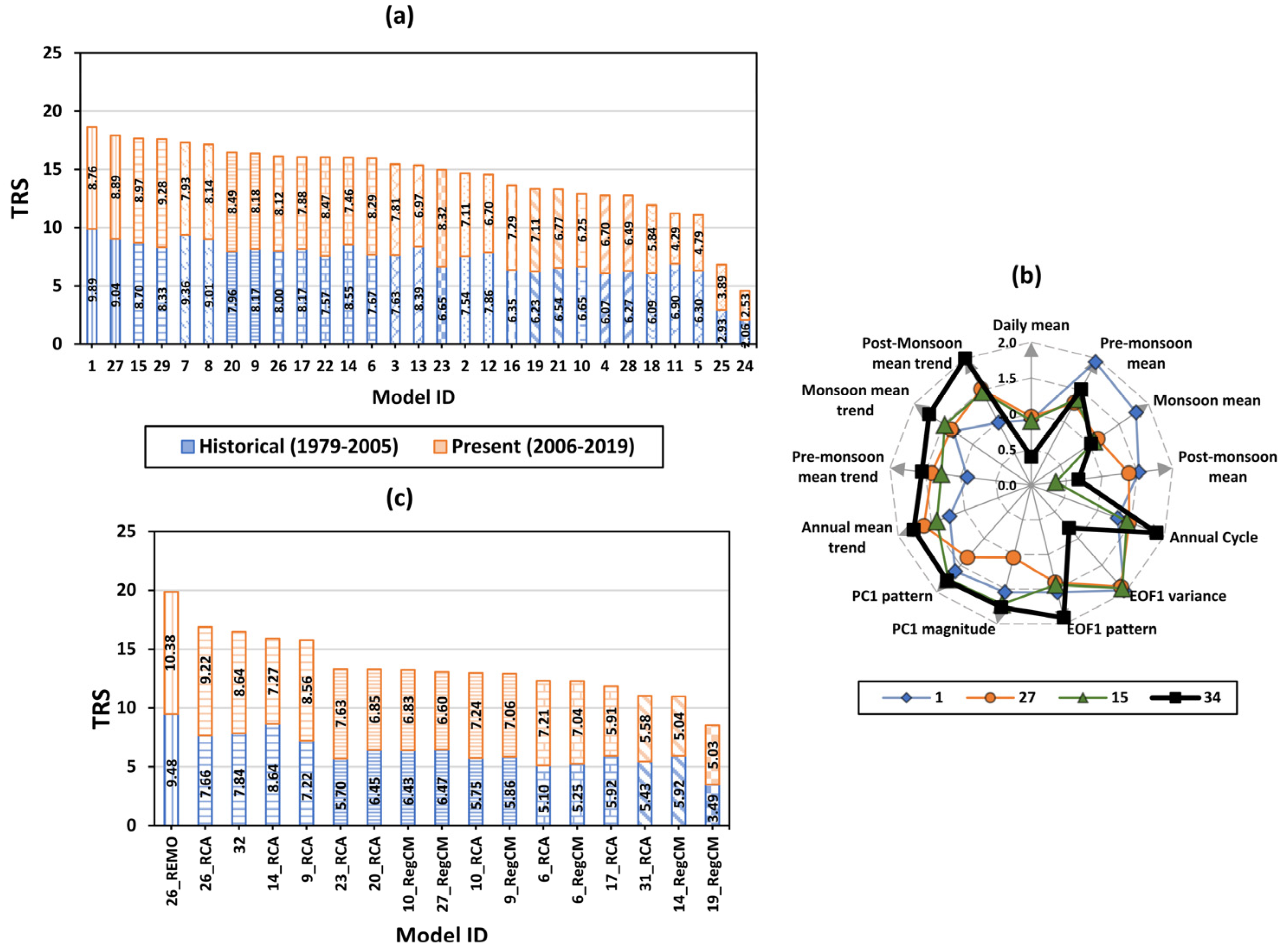
3.2. Construction of Best-Performing Models
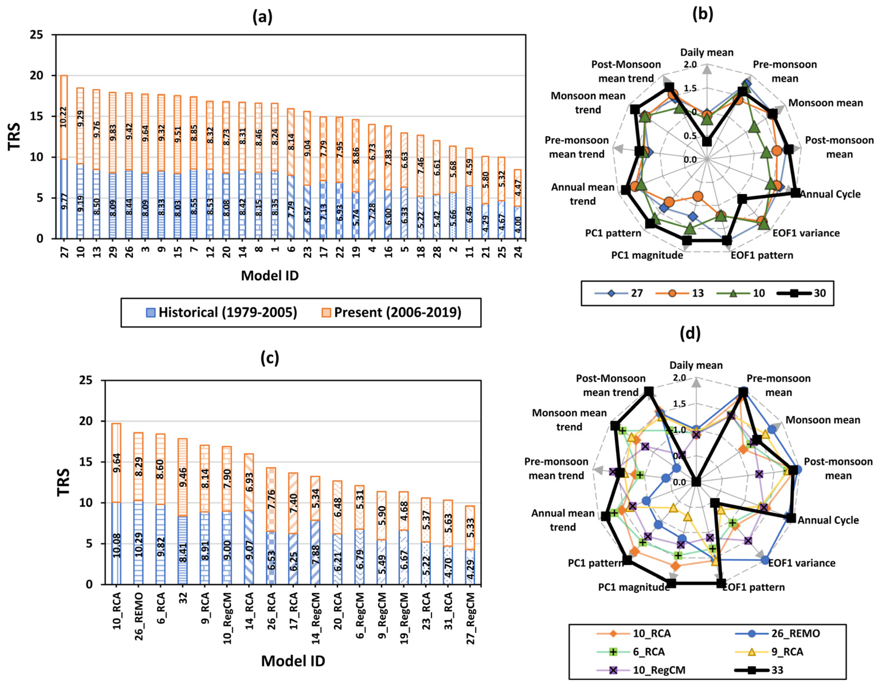
Even though the climate models’ skills were different over climate variable scales, there were a few models that consistently performed well over most of the climate variable scales. To identify those models, the computed Relative Score in each climate variable scale was added together as per Equation (2) to obtain the Total Relative Score (TRS). The estimated TRS of all CMIP5 GCMs and CORDEX RCMs is summarized in Figure 8 and Figure 9. In this study, an attempt was made to determine the number of climate models that should be incorporated while building an ensemble model. The climate models were first separated into the optimal number of groups based on the estimated TRS using the k-mean clustering with silhouette score criterion. Further, the two-sample t-test was used to test whether the groups were statistically significantly different from each other or not at a significant level of 5%. For example, the skill of CMIP5 GCMs was evaluated over the ocean and divided into twelve groups with an average silhouette score of 0.90 (Figure 8a). Model 27 showed very good skill, followed by group 2 models (model 10 and 13) (Figure 8a). The two-sample t-test was used to test whether model 27 was statistically significantly different from group 2 (model 10 and 13) or not. The result indicates that there was no statistically significant difference between group 1 and 2 with a p-value of 0.0737. Hence, the first two groups of climate models were merged to form a new cluster (models 27, 10 and 13). Further, it was found that the new cluster was statistically significantly different from group 3 with a p-value of 0.0136. As suggested by several works of literature, multi-model ensemble climate models performed better than individual climate models, the skill of the climate model constructed from the mean ensemble of the top three CMIP5 GCMs (model 30) was assessed and greater improvements were observed in all climate variable scales, except in capturing the frequency distribution of the daily mean WS and EOF1 variance (Figure 8b). The TRS of constructed climate model 30 was 4.2% higher than model 27 (Figure 8e). A similar analysis as mentioned earlier was carried out for CORDEX RCMs and found that the resultant cluster from the first five group models (group 1:10_RCA, group 2: 26_REMO and 6_RCA, group 3: 32, group 4: 9_RCA and 10_RegCM, and group 5:14_RCA) was statistically significantly different from group 6 with a p-value of 0.039. Since the 14_RCA model has not performed well in the present time slice (Figure 7c), unlike other models, the model 33 was constructed from the ensemble of five top-performing CORDEX RCMs (10_RCA, 26_REMO, 6_RCA, 9_RCA and 10_RegCM) over the ocean in both time slices. Model 33 performed well relative to all individual CORDEX RCMs over the ocean and had a 10.54% higher TRS than 10_RCA (Figure 8d). No individual RCM or GCM was found to perform well in capturing the mean WS trend, whereas the models constructed from top-performing models (model 30 and model 33) showed considerable improvement in capturing the observed mean WS trend over the ocean (Figure 8b,d).
Over land, the CMIP5 GCMs were divided into seventeen groups with an average silhouette score of 0.96 (Figure 9a). Not even a single model consistently performed well in all climate variable scales. Models 1, 27 and 15 showed relatively better skill in some of the climate variable scales. Model 1 showed better performance than 27 and 15 in reproducing seasonal mean WS, whilst the seasonal and annual mean WS trend was well captured by models 27 and 15 compared to model 1 (Figure 9b). The two-sample t-test was used to evaluate whether models 1 and 27 were statistically significantly different from group 3 (models 15 and 29) or not. It was found that there was no statistically significant difference between the model 27 and group 3 with a p-value of 0.1049, so the model 27 could be added to group 3. A statistically significant (p-value of 0.042) difference was observed between model 1 and new group 3 (27, 15 and 29). Since the p-value was close to 0.05 (assumed significant level), and to obtain an added advantage of these models, the ensemble of all these three models’ (with Model ID 34) skill was also evaluated. The results are not as expected in reproducing seasonal mean WS, but an improvement was observed in capturing annual and seasonal mean WS trends. In the case of CORDEX RCMs’ skill over land, 26_REMO was good at reproducing the wind climate well over both the time slices compared to all individual CORDEX RCMs, and it was statistically significantly different from group 2 (26_RCA, 32, 14_RCA and 9_RCA) with a p-value of 0.0081 (Figure 9c). Moreover, the 26_REMO was the only individual RCM that showed good skill over ocean and land.
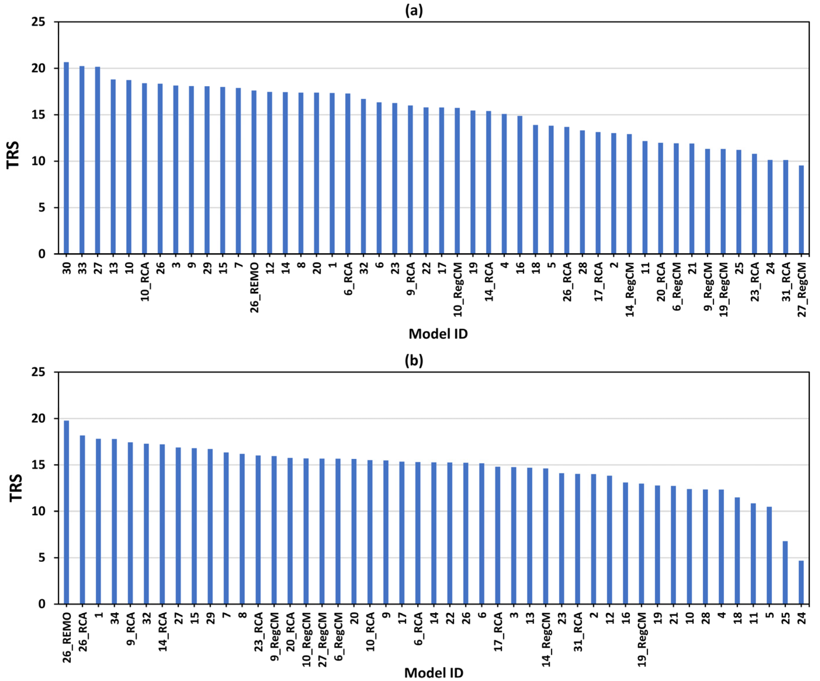
The estimated TRS of all climate models along with the best-performing models over the SA domain are shown in Figure 10. It was observed that the ranking of climate models is controlled by the assessment criteria chosen. So, by comparing the rank awarded to a model without considering the individual assessment criteria as one scenario, the sensitivity of the model rank with individual assessment criteria was explored. It was found that the best-performing models’ (model 30 over ocean; 26_REMO over land) and worst-performing models’ (27_RegCM over ocean; models 24 and 25 over land) ranks are the least sensitive to the chosen assessment criteria (Figures S2 and S3).
3.3. Inter-Comparison of CMIP5 GCMs and CORDEX RCMs
The best-performing climate models in simulating the WS climate over the SA domain were constructed from CMIP5 GCMs and CORDEX RCMs. Now, to answer whether the high-resolution CORDEX RCM performs better than low-resolution CMIP5 GCMs in simulating the WS over the SA domain, we conducted the inter-comparison of climate models. Over the ocean, all the parent GCMs showed higher skill compared to all RCMs, except for 6_RCA (Figure 10a). Chowdhury and Behera [7] used the bias-corrected WS from four CMIP5 GCMs and four CORDEX RCMs as a driving force to the numerical wave model to hindcast the wave climate over the IO, and they also found that ensemble GCMs outperform ensemble RCMs. Therefore, presuming RCMs will simulate the regional climate better than GCMs over the ocean and using them in an impact assessment without explicit evaluation is strongly discouraged. However, over SA land, all the RCMs (except 27_RegCM and 17_RCA) showed higher skill compared to the parent GCMs (Figure 10b). This highlights the added value of using higher spatial resolution RCMs over land. Feser et al. [88] showed that the advantage of using dynamical downscaling regional models compared to driven global climate models in simulating WS can be seen only over complex orographic and coastal areas, unlike over the open ocean. A considerable improvement was observed from the ensemble of best-performing models over the ocean, irrespective of the type of climate model (GCM/RCM) used in the ensemble. Moreover, the best-performing models (model 30 and model 33) over the ocean differed only by 2.1% in the TRS. However, over the land, no added value was observed from the ensemble of the best-performing model (model 34), but it was close to the top-performing GCM (model 1). Thus, the meticulous construction of an ensemble model after the rigorous analysis of individual model potential is important rather than the type of climate model being used (whether it is GCM or RCM).
The selection of RCM based on the parent GCM’s performance for wind-driven process modelling over the ocean is not recommended because most of the parent GCMs outperform the RCMs over the ocean. For example, 27_RegCM is the worst-performing RCM, which is driven by the best-performing GCM (model 27) (Figure 10a). Most of the studies over the SA domain used the WS from climate models without explicitly evaluating their skill in understanding the impact of climate change on the future wave climate, shoreline evolution and assessment of future wind energy potential [89,90,91,92,93]. It is recommended and worth reinvestigating the aforementioned studies using the identified best-performing climate model from this study to reduce the model-based uncertainty. Models 24 (MIROC-ESM) and 25 (MIROC-ESM-CHEM) showed very poor skill relative to all climate models, and a similar skill of the aforementioned models was reported by Tian et al. [86] over the Northern Hemisphere. Therefore, it is strongly recommended not to use MIROC-ESM and MIROC-ESM-CHEM WS projections in climate change impact studies over the SA domain.
In addition to quantifying the skill of climate models, it is important to understand and investigate the root causes behind the difference in skill of climate models. For example, Kunz et al. [34] analyzed the WS from two RCMs and found that the Consortium for Small-Scale Modelling Climate Local Model (COSMO CCLM) is underestimating the intense wind (>8 Bft) due to the lack of physics-based gust parameterization compared to the Regional Model (REMO). Kulkarni et al. [46] assessed the performance of three RCMs and their driving GCMs in simulating offshore wind climate along the Indian coast and attributed the inability of CORDEX RCMs to the lack of land-atmosphere-sea coupling compared to the parent GCMs. Even though the Roosby Centre Regional Atmospheric (RCA) and Regional Climatic Model (RegCM) type RCMs had a similar spatial resolution, the RCA type RCMs performed better in simulating WS than the RegCM type RCMs over both the ocean and land of the SA domain, and this can be attributed to the difference in model configuration (Figure 10). The details about RCA and RegCM models are presented in Samuelsson et al. [94] and Giorgi et al. [95], respectively. Even when simulating precipitation, four RCMs differed in skill, despite being forced with the same lateral boundary conditions [37]. Thus, the model configuration could play a more major role than the spatial resolution itself. In the current study, we assessed the skill of thirteen Earth System Models (ESMs), two ChemESMs and thirteen Atmospheric-Ocean GCMs (AOGCMs); it was expected that ESMs should perform well compared to AOGCMs as it considered the higher number of processes and more dynamical components. Interestingly, the top-performing individual GCMs in representing the WS over the SA ocean and land were ESM (27-MPI-ESM-MR) and AOGCM (1-ACCESS1.0), respectively. On the other hand, the worst-performing model was ESM (model 24). Desmet and Ngo-Duc [85] evaluated the skill of CMIP6 GCMs, and it was observed that ACCESS-CM2 (AOGCM) had a higher skill score than ACCESS-ESM1 (ESM) in representing precipitation and 850 hPa wind over South East Asia. This led to the question of what specifically in the model configuration attributed to the skill of GCMs in representing WS. A recent study by Morim et al. [50] found that improving the atmospheric component results in a greater reduction in WS bias compared to the land surface component, ocean component, sea-ice component, land-carbon and ocean-carbon components of the particular GCM. Since the added advantage of the carbon-cycle component is not reflected in the simulation of WS, Morim et al. [50] expected no major change in the WS simulation of CMIP6 GCMs (with the carbon-cycle component) at decadal time slices. In contrast, Krishnan and Bhaskaran [43] found a significant improvement in CMIP6 GCMs’ WS simulation over BoB compared to CMIP5 GCMs. This indeed requires more attention for analyzing each climate model’s configuration using the estimated skill to answer the contribution of each dynamical component in representing WS. In this study, the relative skill of CMIP5 GCMs and CORDEX RCMs in representing WS over the SA domain is presented. However, analyzing the skill of climate models by generating spatial bias maps in each climate variable scale will aid in identifying where the particular climate model shows significant bias. Then, the mechanisms responsible for bias over a region can be studied by examining the spatial variability maps of sea level pressure, sea surface temperature and surface air temperature [37,82,96].
4. Conclusions
This paper assessed the skill of all available sixteen CORDEX RCMs and twenty-eight CMIP5 GCMs in simulating near-surface wind speed (WS) over the South Asian (SA) domain using the developed Total Relative Score method. Further, to answer whether the RCMs showed any benefit in simulating WS rather than their parent GCMs, the inter-comparison between RCMs and GCMs was carried out. The ability of the climate model’s performance was assessed relative to ERA5 in representing the entire domain frequency density of daily mean WS, capturing the annual cycle WS pattern, reproducing the mean and trend of annual and seasonal mean WS and finally in reproducing the dominant variation pattern of monthly mean WS using suitable assessment criteria. The following conclusions are drawn from this study:
- Over the SA domain, model 30 (constructed from mean ensemble of MPI-ESM-MR, CSIRO-Mk3.6.0 and GFDL-ESM2G GCMs) and REMO2009 RCM driven by MPI-M-MPI-ESM-LR GCM perform well over ocean and land, respectively.
- It is recommended to use the WS projections constructed from the mean ensemble of MPI-ESM-MR, CSIRO-Mk3.6.0 and GFDL-ESM2G GCMs for understanding the impact of climate change on future wave climate, coastal sediment transport and offshore wind energy potential over the SA ocean region. However, the individual GCMs can also be used with caution.
- Over the SA land region, the REMO2009 RCM driven by MPI-M-MPI-ESM-LR GCM WS projections can be used for assessing climate change impact studies on evapotranspiration, onshore wind energy potential and air pollution modelling.
- MIROC-ESM and MIROC-ESM-CHEM GCMs show very poor skill in representing WS over SA ocean and land regions, and these GCMs are strongly not recommended in understanding the wind-driven processes.
- All the parent GCMs show higher skill compared to all RCMs, except for 6_RCA, over the SA ocean region. Conversely, over the SA land region, all the RCMs (except 27_RegCM and 17_RCA) show higher skill compared to the parent GCMs. This concludes that the RCMs show significant added value over land, unlike over the open ocean.
- Most of the parent GCMs outperform the RCMs over the SA ocean region. Using the RCM WS projections based on the corresponding parent GCM performance in wind-driven models for climate change impact and policymaking is strongly not recommended.
- The ensemble of all climate models need not be always considered as reliable. However, the meticulous construction of the ensemble model after the rigorous analysis of individual model potential is important, rather than the type of climate model being used (whether it is GCM or RCM).
- It is observed that improving spatial resolution itself does not improve the climate model skill, whereas model configuration plays a key role. Further, in addition to quantifying GCM competence, it is critical to comprehend the benefit/disadvantage added by integrating more dynamical processes (such as carbon cycle dynamics and bio-geochemical processes) in WS simulation.
A detailed study on understanding the WS spatial bias pattern, investigating the contribution of different dynamical components in representing accurate WS and analyzing the future changes in WS pattern over the SA domain will be addressed separately for CORDEX RCMs and CMIP5 GCMs in a future study.
Supplementary Materials
The following supporting information can be downloaded at: https://0-www-mdpi-com.brum.beds.ac.uk/article/10.3390/cli10060085/s1, Table S1: The Relative Score (RS) of each climate model (in descending order) in representing the frequency distribution of daily mean near-surface wind speed over the South Asian Ocean and Land (Note: Here RS is out of 1, which is the summation of historical time slice RS and present time slice RS); Table S2: The Relative Score (RS) of each climate model (in descending order) in representing spatio-temporal variability of the monthly mean near-surface wind speed over the South Asian Ocean and Land (Note: Here RS is out of 8, which is the summation of climate model RS in representing EOF1 variance and pattern, and PC1 magnitude and pattern for both study time slices); Table S3: The Relative Score (RS) of each climate model (in descending order) in capturing the annual cycle variation over the South Asian Ocean and Land (Note: Here RS is out of 2, which is the summation of historical time slice RS and present time slice RS); Table S4: The Relative Score (RS) of each climate model (in descending order) in reproducing the seasonal mean wind speed over the South Asian Ocean and Land (Note: Here RS is out of 6, which is the summation of RS of a climate model in pre-monsoon, monsoon and post-monsoon seasons for both study time slices); Table S5: The Relative Score (RS) of each climate model (in descending order) in reproducing the pre-monsoon mean wind speed trend over the South Asian Ocean and Land (Note: Here RS is out of 2, which is the summation of the historical time slice RS and present time slice RS); Table S6: The Relative Score (RS) of each climate model (in descending order) in reproducing the monsoon mean wind speed trend over the South Asian Ocean and Land (Note: Here RS is out of 2, which is the summation of historical time slice RS and present time slice RS); Table S7: The Relative Score (RS) of each climate model (in descending order) in reproducing the post-monsoon mean wind speed trend over the South Asian Ocean and Land (Note: Here RS is out of 2, which is the summation of the historical time slice RS and present time slice RS); Table S8: The Relative Score (RS) of each climate model (in descending order) in reproducing the seasonal mean wind speed trend over the South Asian Ocean and Land (Note: Here RS is out of 6, which is the summation of RS of a climate model in pre-monsoon, monsoon and post-monsoon seasons for both study time slices); Table S9: The Relative Score (RS) of each climate model (in descending order) in reproducing the annual mean wind speed trend over the South Asian Ocean and Land (Note: Here RS is out of 2, which is the summation of the historical time slice RS and present time slice RS). Figure S1: Pre-monsoon (February–May) mean wind speed spatial maps of ERA5 for the (a) historical (1979–2005) and (b) present time slice (2006–2019). (c) Percentage change of present time slice pre-monsoon mean wind speed relative to historical time slice pre-monsoon mean wind speed (Δ, %). (d–f) As in (a–c), but for the monsoon season (June–September). (g–i) As in (a–c), but for the post-monsoon season (October–January); Figure S2: Sensitivity of climate model’s rank with chosen assessment criteria over ocean part of South Asian domain. Climate model rank obtained by removing a specific assessment criterion are marked with right pointed triangle markers for without evaluating daily mean wind speed, square markers for without evaluating the seasonal mean wind speed, diamond markers for without evaluating the long-term monthly mean wind speed pattern (annual cycle), left pointed triangle markers for without consideration of the Empirical Orthogonal Function (EOF) analysis, cross sign markers for without evaluating the annual mean wind speed trend and plus sign markers for without evaluating seasonal mean wind speed trend. The bubble size indicates the total of how many cases (out of 7) have given a particular rank to the climate model. For example, model 30 has secured the first rank in 6 cases (except without the seasonal mean trend case). The thick black line is the result case obtained by considering all the assessment criteria and it passes through the largest bubble for 36 ranks out of 48. The interchange of rank is observed between the climate models whose Total Relative Score is near to each other. Figure S3: As in Figure S2, but for over the land part of the South Asian domain. For example, model 26_REMO has secured the first rank in 6 cases (except without the seasonal mean case). However, models 24 and 25 have secured 47 and 46, respectively in all 7 cases.
Author Contributions
Conceptualization, N.K.G.L. and M.R.B.; Data curation, N.K.G.L. and M.R.B.; Formal analysis, N.K.G.L. and M.R.B.; Methodology, N.K.G.L. and M.R.B.; Resources, N.K.G.L. and M.R.B.; Software, N.K.G.L. and M.R.B.; Supervision, M.R.B.; Validation, N.K.G.L. and M.R.B.; Visualization, N.K.G.L. and M.R.B.; Writing—original draft, N.K.G.L.; Writing—review and editing, N.K.G.L. and M.R.B. All authors have read and agreed to the published version of the manuscript.
Funding
This research received no external funding.
Institutional Review Board Statement
Not applicable.
Informed Consent Statement
Not applicable.
Data Availability Statement
The daily mean WS zonal and meridional components are publicly available from the Earth System Grid Federation portal (https://esg-dn1.nsc.liu.se/search/cordex/, accessed on 1 January 2020 and https://esgf-node.llnl.gov/search/cmip5/, accessed on 11 January 2021). The ERA5 WS of European Centre for Medium Range Weather Forecasts is also publicly available from Copernicus Climate Change Service Climate Date Store (https://cds.climate.copernicus.eu/, accessed on 1 January 2020).
Acknowledgments
The authors acknowledge the World Climate Research Program’s Working Group on forming the CORDEX and CMIP5 framework and making the climate model outputs available. The authors also acknowledge the European Centre for Medium Range Weather Forecasts for providing the ERA5 wind dataset.
Conflicts of Interest
The authors declare no conflict of interest.
References
- Yang, L.; Feng, Q.; Adamowski, J.F.; Yin, Z.; Wen, X.; Wu, M.; Jia, B.; Hao, Q. Erratum to ‘Spatio-temporal variation of reference evapotranspiration in northwest China based on CORDEX-EA’ [Atmos. Res. 238 (2020) 104868]. Atmos. Res. 2021, 252, 105425. [Google Scholar] [CrossRef]
- Ottosen, T.B.; Ketzel, M.; Skov, H.; Hertel, O.; Brandt, J.; Kakosimos, K.E. Micro-scale modelling of the urban wind speed for air pollution applications. Sci. Rep. 2019, 9, 14279. [Google Scholar] [CrossRef] [PubMed] [Green Version]
- Ottosen, T.B.; Ketzel, M.; Skov, H.; Hertel, O.; Brandt, J.; Kakosimos, K.E. A parameter estimation and identifiability analysis methodology applied to a street canyon air pollution model. Environ. Model. Softw. 2016, 84, 165–176. [Google Scholar] [CrossRef]
- Kulkarni, S.; Deo, M.C.; Ghosh, S. Framework for assessment of climate change impact on offshore wind energy. Meteorol. Appl. 2017, 25, 94–104. [Google Scholar] [CrossRef] [Green Version]
- Nabipour, N.; Mosavi, A.; Hajnal, E.; Nadai, L.; Shamshirband, S.; Chau, K.W. Modeling climate change impact on wind power resources using adaptive neuro-fuzzy inference system. Eng. Appl. Comput. Fluid Mech. 2020, 14, 491–506. [Google Scholar] [CrossRef] [Green Version]
- Hemer, M.A.; Trenham, C.E. Evaluation of a CMIP5 derived dynamical global wind wave climate model ensemble. Ocean Model. 2016, 103, 190–203. [Google Scholar] [CrossRef] [Green Version]
- Chowdhury, P.; Behera, M.R. Evaluation of CMIP5 and CORDEX derived wave climate in Indian Ocean. Clim. Dyn. 2018, 52, 4463–4482. [Google Scholar] [CrossRef]
- Chowdhury, P.; Behera, M.R.; Reeve, D.E. Wave climate projections along the Indian coast. Int. J. Climatol. 2019, 39, 4531–4542. [Google Scholar] [CrossRef] [Green Version]
- Fan, Y.; Lin, S.J.; Griffies, S.M.; Hemer, M.A. Simulated global swell and wind-sea climate and their responses to anthropogenic climate change at the end of the twenty-first century. J. Clim. 2014, 27, 3516–3536. [Google Scholar] [CrossRef]
- Chowdhury, P.; Behera, M.R. Nearshore Sediment Transport in a Changing Climate. In Climate Change Signals and Response: A Strategic Knowledge Compendium for India; Venkataraman, C., Mishra, T., Ghosh, S., Karmakar, S., Eds.; Springer Singapore: Singapore, 2019; pp. 147–160. ISBN 978-981-13-0280-0. [Google Scholar]
- Rajasree, B.R.; Deo, M.C. Evaluation of estuary shoreline shift in response to climate change: A study from the central west coast of India. L. Degrad. Dev. 2018, 29, 3571–3583. [Google Scholar] [CrossRef]
- Munk, W.; Wunsch, C. Abyssal recipes II: Energetics of tidal and wind mixing. Deep Sea Res. Part I Oceanogr. Res. Pap. 1998, 45, 1977–2010. [Google Scholar] [CrossRef]
- Hemer, M.A.; McInnes, K.L.; Ranasinghe, R. Climate and variability bias adjustment of climate model-derived winds for a southeast Australian dynamical wave model. Ocean Dyn. 2012, 62, 87–104. [Google Scholar] [CrossRef]
- Macias, D.; Garcia-Gorriz, E.; Dosio, A.; Stips, A.; Keuler, K. Obtaining the correct sea surface temperature: Bias correction of regional climate model data for the Mediterranean Sea. Clim. Dyn. 2018, 51, 1095–1117. [Google Scholar] [CrossRef] [Green Version]
- Colbert, A.J.; Soden, B.J.; Kirtman, B.P. The impact of natural and anthropogenic climate change on western North Pacific tropical cyclone tracks. J. Clim. 2015, 28, 1806–1823. [Google Scholar] [CrossRef]
- Shimura, T.; Mori, N.; Mase, H. Future projection of ocean wave climate: Analysis of SST impacts on wave climate changes in the Western North Pacific. J. Clim. 2015, 28, 3171–3190. [Google Scholar] [CrossRef] [Green Version]
- Burke, C.; Stott, P. Impact of anthropogenic climate change on the East Asian summer monsoon. J. Clim. 2017, 30, 5205–5220. [Google Scholar] [CrossRef]
- Davy, R.; Outten, S. The arctic surface climate in CMIP6: Status and developments since CMIP5. J. Clim. 2020, 33, 8047–8068. [Google Scholar] [CrossRef]
- Krishnan, A.; Bhaskaran, P.K.; Kumar, P. CMIP5 model performance of significant wave heights over the Indian Ocean using COWCLIP datasets. Theor. Appl. Climatol. 2021, 145, 377–392. [Google Scholar] [CrossRef]
- Saha, A.; Ghosh, S.; Sahana, A.S.; Rao, E.P. Failure of CMIP5 climate models in simulating post-1950 decreasing trend of Indian monsoon. Geophys. Res. Lett. 2014, 41, 7323–7330. [Google Scholar] [CrossRef]
- Trzaska, S.; Schnarr, E. A Review of Downscaling Methods for Climate Change Projections; United States Agency for International Development: Washington, DC, USA, 2014. [Google Scholar]
- Önol, B.; Bozkurt, D.; Turuncoglu, U.U.; Sen, O.L.; Dalfes, H.N. Evaluation of the twenty-first century RCM simulations driven by multiple GCMs over the Eastern Mediterranean-Black Sea region. Clim. Dyn. 2014, 42, 1949–1965. [Google Scholar] [CrossRef]
- Mori, N.; Shimura, T.; Yasuda, T.; Mase, H. Multi-model climate projections of ocean surface variables under different climate scenarios-Future change of waves, sea level and wind. Ocean Eng. 2013, 71, 122–129. [Google Scholar] [CrossRef]
- Wang, X.L.; Feng, Y.; Swail, V.R. Changes in global ocean wave heights as projected using multimodel CMIP5 simulations. Geophys. Res. Lett. 2014, 41, 1026–1034. [Google Scholar] [CrossRef]
- Perez, J.; Menendez, M.; Camus, P.; Mendez, F.J.; Losada, I.J. Statistical multi-model climate projections of surface ocean waves in Europe. Ocean Model. 2015, 96, 161–170. [Google Scholar] [CrossRef]
- Grabemann, I.; Weisse, R. Climate change impact on extreme wave conditions in the north sea: An ensemble study. Ocean Dyn. 2008, 58, 199–212. [Google Scholar] [CrossRef] [Green Version]
- Hemer, M.A.; Fan, Y.; Mori, N.; Semedo, A.; Wang, X.L. Projected changes in wave climate from a multi-model ensemble. Nat. Clim. Chang. 2013, 3, 471–476. [Google Scholar] [CrossRef]
- Pinto, I.; Lennard, C.; Tadross, M.; Hewitson, B.; Dosio, A.; Nikulin, G.; Panitz, H.J.; Shongwe, M.E. Evaluation and projections of extreme precipitation over southern Africa from two CORDEX models. Clim. Change 2016, 135, 655–668. [Google Scholar] [CrossRef] [Green Version]
- Abba Omar, S.; Abiodun, B.J. How well do CORDEX models simulate extreme rainfall events over the East Coast of South Africa? Theor. Appl. Climatol. 2017, 128, 453–464. [Google Scholar] [CrossRef]
- Choudhary, A.; Dimri, A.P.; Maharana, P. Assessment of CORDEX-SA experiments in representing precipitation climatology of summer monsoon over India. Theor. Appl. Climatol. 2018, 134, 283–307. [Google Scholar] [CrossRef]
- Gbobaniyi, E.; Sarr, A.; Sylla, M.B.; Diallo, I.; Lennard, C.; Dosio, A.; Dhiédiou, A.; Kamga, A.; Klutse, N.A.B.; Hewitson, B.; et al. Climatology, annual cycle and interannual variability of precipitation and temperature in CORDEX simulations over West Africa. Int. J. Climatol. 2014, 34, 2241–2257. [Google Scholar] [CrossRef]
- Spinoni, J.; Barbosa, P.; Bucchignani, E.; Cassano, J.; Cavazos, T.; Christensen, J.H.; Christensen, O.B.; Coppola, E.; Evans, J.; Geyer, B.; et al. Future global meteorological drought hot spots: A study based on CORDEX data. J. Clim. 2020, 33, 3635–3661. [Google Scholar] [CrossRef]
- Dafka, S.; Toreti, A.; Luterbacher, J.; Zanis, P.; Tyrlis, E.; Xoplaki, E. On the ability of RCMs to capture the circulation pattern of Etesians. Clim. Dyn. 2018, 51, 1687–1706. [Google Scholar] [CrossRef]
- Kunz, M.; Mohr, S.; Rauthe, M.; Lux, R.; Kottmeier, C. Assessment of extreme wind speeds from regional climate models-Part 1: Estimation of return values and their evaluation. Nat. Hazards Earth Syst. Sci. 2010, 10, 907–922. [Google Scholar] [CrossRef] [Green Version]
- Rockel, B.; Woth, K. Extremes of near-surface wind speed over Europe and their future changes as estimated from an ensemble of RCM simulations. Clim. Change 2007, 81, 267–280. [Google Scholar] [CrossRef] [Green Version]
- Iizuka, S.; Dairaku, K.; Sasaki, W.; Adachi, S.A.; Ishizaki, N.N.; Kusaka, H.; Takayabu, I. Assessment of ocean surface winds and tropical cyclones around Japan by RCMs. J. Meteorol. Soc. Japan 2012, 90, 91–102. [Google Scholar] [CrossRef] [Green Version]
- Lucas-Picher, P.; Christensen, J.H.; Saeed, F.; Kumar, P.; Asharaf, S.; Ahrens, B.; Wiltshire, A.J.; Jacob, D.; Hagemann, S. Can regional climate models represent the Indian monsoon? J. Hydrometeorol. 2011, 12, 849–868. [Google Scholar] [CrossRef] [Green Version]
- Winterfeldt, J.; Weisse, R. Assessment of value added for surface marine wind speed obtained from two regional climate models. Mon. Weather Rev. 2009, 137, 2955–2965. [Google Scholar] [CrossRef] [Green Version]
- Krishnan, A.; Bhaskaran, P.K. Performance of CMIP5 wind speed from global climate models for the Bay of Bengal region. Int. J. Climatol. 2020, 40, 3398–3416. [Google Scholar] [CrossRef]
- Mohan, S.; Bhaskaran, P.K. Evaluation of CMIP5 climate model projections for surface wind speed over the Indian Ocean region. Clim. Dyn. 2019, 53, 5415–5435. [Google Scholar] [CrossRef]
- Krishnan, A.; Bhaskaran, P.K. CMIP5 wind speed comparison between satellite altimeter and reanalysis products for the Bay of Bengal. Environ. Monit. Assess. 2019, 191, 554. [Google Scholar] [CrossRef]
- Mohan, S.; Bhaskaran, P.K. Evaluation and bias correction of global climate models in the CMIP5 over the Indian Ocean region. Environ. Monit. Assess. 2019, 191, 806. [Google Scholar] [CrossRef]
- Krishnan, A.; Bhaskaran, P.K. Skill assessment of global climate model wind speed from CMIP5 and CMIP6 and evaluation of projections for the Bay of Bengal. Clim. Dyn. 2020, 55, 2667–2687. [Google Scholar] [CrossRef]
- Torma, C.; Giorgi, F.; Coppola, E. Added value of regional climate modeling over areas characterized by complex terrain-precipitation over the Alps. J. Geophys. Res. 2015, 120, 3957–3972. [Google Scholar] [CrossRef]
- Singh, S.; Ghosh, S.; Sahana, A.S.; Vittal, H.; Karmakar, S. Do dynamic regional models add value to the global model projections of Indian monsoon? Clim. Dyn. 2017, 48, 1375–1397. [Google Scholar] [CrossRef]
- Kulkarni, S.; Deo, M.C.; Ghosh, S. Performance of the CORDEX regional climate models in simulating offshore wind and wind potential. Theor. Appl. Climatol. 2018, 135, 1449–1464. [Google Scholar] [CrossRef]
- Raju, K.S.; Kumar, D.N. Review of approaches for selection and ensembling of GCMS. J. Water Clim. Chang. 2020, 11, 577–599. [Google Scholar] [CrossRef]
- Srinivasa Raju, K.; Nagesh Kumar, D. Ranking general circulation models for India using TOPSIS. J. Water Clim. Chang. 2015, 6, 288–299. [Google Scholar] [CrossRef] [Green Version]
- Raju, K.S.; Kumar, D.N. Ranking of global climate models for India using multicriterion analysis. Clim. Res. 2014, 60, 103–117. [Google Scholar] [CrossRef]
- Morim, J.; Hemer, M.; Andutta, F.; Shimura, T.; Cartwright, N. Skill and uncertainty in surface wind fields from general circulation models: Intercomparison of bias between AGCM, AOGCM and ESM global simulations. Int. J. Climatol. 2020, 40, 2659–2673. [Google Scholar] [CrossRef]
- Herrmann, M.; Somot, S.; Calmanti, S.; Dubois, C.; Sevault, F. Representation of spatial and temporal variability of daily wind speed and of intense wind events over the Mediterranean Sea using dynamical downscaling: Impact of the regional climate model configuration. Nat. Hazards Earth Syst. Sci. 2011, 11, 1983–2001. [Google Scholar] [CrossRef] [Green Version]
- De Winter, R.C.; Sterl, A.; Ruessink, B.G. Wind extremes in the North Sea Basin under climate change: An ensemble study of 12 CMIP5 GCMs. J. Geophys. Res. Atmos. 2013, 118, 1601–1612. [Google Scholar] [CrossRef] [Green Version]
- Gallagher, S.; Gleeson, E.; Tiron, R.; McGrath, R.; Dias, F. Twenty-first century wave climate projections for Ireland and surface winds in the North Atlantic Ocean. Adv. Sci. Res. 2016, 13, 75–80. [Google Scholar] [CrossRef] [Green Version]
- Alizadeh, M.J.; Kavianpour, M.R.; Kamranzad, B.; Etemad-Shahidi, A. A Weibull Distribution Based Technique for Downscaling of Climatic Wind Field. Asia-Pacific J. Atmos. Sci. 2019, 55, 685–700. [Google Scholar] [CrossRef]
- Abolude, A.T.; Zhou, W.; Akinsanola, A.A. Evaluation and projections of wind power resources over China for the energy industry using CMIP5 models. Energies 2020, 13, 2417. [Google Scholar] [CrossRef]
- Wang, X.L.; Swail, V.R.; Cox, A. Dynamical versus statistical downscaling methods for ocean wave heights. Int. J. Climatol. 2009, 30, 317–332. [Google Scholar] [CrossRef]
- Li, D.; Staneva, J.; Grayek, S.; Behrens, A.; Feng, J.; Yin, B. Skill assessment of an atmosphere-wave regional coupled model over the east china sea with a focus on typhoons. Atmosphere 2020, 11, 252. [Google Scholar] [CrossRef] [Green Version]
- Muhammed Naseef, T.; Sanil Kumar, V. Climatology and trends of the Indian Ocean surface waves based on 39-year long ERA5 reanalysis data. Int. J. Climatol. 2020, 40, 979–1006. [Google Scholar] [CrossRef]
- Costoya, X.; de Castro, M.; Carvalho, D.; Feng, Z.; Gómez-Gesteira, M. Climate change impacts on the future offshore wind energy resource in China. Renew. Energy 2021, 175, 731–747. [Google Scholar] [CrossRef]
- Saenz-Aguirre, A.; Saenz, J.; Ulazia, A.; Ibarra-Berastegui, G. Optimal strategies of deployment of far offshore co-located wind-wave energy farms. Energy Convers. Manag. 2022, 251, 114914. [Google Scholar] [CrossRef]
- Zhao, L.; Jin, S.; Liu, X.; Wang, B.; Song, Z.; Hu, J.; Guo, Y. Assessment of CMIP6 Model Performance for Wind Speed in China. Front. Clim. 2021, 3, 1–8. [Google Scholar] [CrossRef]
- Molina, M.O.; Gutiérrez, C.; Sánchez, E. Comparison of ERA5 surface wind speed climatologies over Europe with observations from the HadISD dataset. Int. J. Climatol. 2021, 41, 4864–4878. [Google Scholar] [CrossRef]
- Olauson, J. ERA5: The new champion of wind power modelling? Renew. Energy 2018, 126, 322–331. [Google Scholar] [CrossRef] [Green Version]
- Hayes, L.; Stocks, M.; Blakers, A. Accurate long-term power generation model for offshore wind farms in Europe using ERA5 reanalysis. Energy 2021, 229, 120603. [Google Scholar] [CrossRef]
- Hersbach, H.; Bell, W.; Berrisford, P.; Horányi, A.J.; Sabater, J.M.; Nicolas, J.; Radu, R.; Schepers, D.; Simmons, A.; Soci, C.; et al. Global reanalysis: Goodbye ERA-Interim, hello ERA5. ECMWF Newsl. 2019, 159, 17–24. [Google Scholar] [CrossRef]
- Belmonte Rivas, M.; Stoffelen, A. Characterizing ERA-Interim and ERA5 surface wind biases using ASCAT. Ocean Sci. 2019, 15, 831–852. [Google Scholar] [CrossRef] [Green Version]
- Minola, L.; Zhang, F.; Azorin-Molina, C.; Pirooz, A.A.S.; Flay, R.G.J.; Hersbach, H.; Chen, D. Near-surface mean and gust wind speeds in ERA5 across Sweden: Towards an improved gust parametrization. Clim. Dyn. 2020, 55, 887–907. [Google Scholar] [CrossRef]
- Parker, K.; Hill, D.F. Evaluation of bias correction methods for wave modeling output. Ocean Model. 2017, 110, 52–65. [Google Scholar] [CrossRef]
- Li, D.; Feng, J.; Xu, Z.; Yin, B.; Shi, H.; Qi, J. Statistical Bias Correction for Simulated Wind Speeds Over CORDEX-East Asia. Earth Sp. Sci. 2019, 6, 200–211. [Google Scholar] [CrossRef]
- Li, H.; Sheffield, J.; Wood, E.F. Bias correction of monthly precipitation and temperature fields from Intergovernmental Panel on Climate Change AR4 models using equidistant quantile matching. J. Geophys. Res. Atmos. 2010, 115, D10. [Google Scholar] [CrossRef]
- Schulzweida, U. CDO User Guide 2021. Available online: https://zenodo.org/record/5614769#.YqlZU-xByUk (accessed on 1 January 2022).
- Jones, P. A User’s Guide for SCRIP: A Spherical Coordinate Remapping and Interpolation Package; Version 1.4; Los Alamos National Laboratory: Los Alamos, NM, USA, 1998. [Google Scholar]
- Perkins, S.E.; Pitman, A.J.; Holbrook, N.J.; McAneney, J. Evaluation of the AR4 climate models’ simulated daily maximum temperature, minimum temperature, and precipitation over Australia using probability density functions. J. Clim. 2007, 20, 4356–4376. [Google Scholar] [CrossRef]
- Kendall, M.G. Rank Correlation Methods. Biometrika 1957, 44, 107–116. [Google Scholar] [CrossRef]
- Mann, H.B. Non-Parametric Test Against Trend. Econometrica 1945, 13, 245–259. [Google Scholar] [CrossRef]
- Sen, P.K. Estimates of the Regression Coefficient Based on Kendall’s Tau. J. Am. Stat. Assoc. 1968, 63, 1379–1389. [Google Scholar] [CrossRef]
- Wang, F.; Shao, W.; Yu, H.; Kan, G.; He, X.; Zhang, D.; Ren, M.; Wang, G. Re-evaluation of the Power of the Mann-Kendall Test for Detecting Monotonic Trends in Hydrometeorological Time Series. Front. Earth Sci. 2020, 8, 1–12. [Google Scholar] [CrossRef]
- Tebaldi, C.; Knutti, R. The use of the multi-model ensemble in probabilistic climate projections. Philos. Trans. R. Soc. A Math. Phys. Eng. Sci. 2007, 365, 2053–2075. [Google Scholar] [CrossRef] [PubMed]
- Thober, S.; Samaniego, L. Robust ensemble selection by multivariate evaluation of extreme precipitation and temperature characteristics. J. Geophys. Res. 2014, 119, 594–613. [Google Scholar] [CrossRef]
- Kulkarni, S.; Deo, M.C.; Ghosh, S. Evaluation of wind extremes and wind potential under changing climate for Indian offshore using ensemble of 10 GCMs. Ocean Coast. Manag. 2016, 121, 141–152. [Google Scholar] [CrossRef]
- Hassan, I.; Kalin, R.M.; White, C.J.; Aladejana, J.A. Selection of CMIP5 GCM ensemble for the projection of spatio-temporal changes in precipitation and temperature over the Niger Delta, Nigeria. Water 2020, 12, 385. [Google Scholar] [CrossRef] [Green Version]
- Herrmann, M.; Nguyen-Duy, T.; Ngo-Duc, T.; Tangang, F. Climate change impact on sea surface winds in Southeast Asia. Int. J. Climatol. 2021, 42, 3571–3595. [Google Scholar] [CrossRef]
- Anoop, T.R.; Kumar, V.S.; Shanas, P.R.; Johnson, G. Surface wave climatology and its variability in the north Indian Ocean Based on ERA-interim reanalysis. J. Atmos. Ocean. Technol. 2015, 32, 1372–1385. [Google Scholar] [CrossRef] [Green Version]
- Müller, W.A.; Jungclaus, J.H.; Mauritsen, T.; Baehr, J.; Bittner, M.; Budich, R.; Bunzel, F.; Esch, M.; Ghosh, R.; Haak, H.; et al. A Higher-resolution Version of the Max Planck Institute Earth System Model (MPI-ESM1.2-HR). J. Adv. Model. Earth Syst. 2018, 10, 1383–1413. [Google Scholar] [CrossRef]
- Desmet, Q.; Ngo-Duc, T. A novel method for ranking CMIP6 global climate models over the southeast Asian region. Int. J. Climatol. 2021, 42, 97–117. [Google Scholar] [CrossRef]
- Tian, Q.; Huang, G.; Hu, K.; Niyogi, D. Observed and Global Climate Model Based Changes in Wind Power Potential over the Northern Hemisphere during 1979–2016; Elsevier Ltd.: Amsterdam, The Netherlands, 2019; Volume 167, ISBN 1082995312. [Google Scholar]
- Shanas, P.R.; Sanil Kumar, V. Temporal variations in the wind and wave climate at a location in the eastern Arabian Sea based on ERA-Interim reanalysis data. Nat. Hazards Earth Syst. Sci. 2014, 14, 1371–1381. [Google Scholar] [CrossRef] [Green Version]
- Feser, F.; Rrockel, B.; Storch, H.; Winterfeldt, J.; Zahn, M. Regional climate models add value to global model data a review and selected examples. Bull. Am. Meteorol. Soc. 2011, 92, 1181–1192. [Google Scholar] [CrossRef] [Green Version]
- Roshin, E.; Deo, M.C. Derivation of design waves along the Indian coastline incorporating climate change. J. Mar. Sci. Technol. 2016, 22, 61–70. [Google Scholar] [CrossRef]
- Bhat, S.; Jain, P.; Deo, M.C. Application of Regional Climate Models for Coastal Design Parameters along India. J. Coast. Res. 2018, 35, 110–121. [Google Scholar] [CrossRef]
- Gopikrishna, B.; Deo, M.C. Changes in the shoreline at Paradip Port, India in response to climate change. Geomorphology 2018, 303, 243–255. [Google Scholar] [CrossRef]
- Jain, P.; Deo, M.C. Climate Change Impact on Design Waves Using Climate Models. In Proceedings of the Fourth International Conference in Ocean Engineering (ICOE2018); Murali, K., Sriram, V., Samad, A., Saha, N., Eds.; Springer: Singapore, 2019; pp. 783–794. [Google Scholar]
- Rajasree, B.R.; Deo, M.C. Assessment of Coastal Vulnerability Considering the Future Climate: A Case Study along the Central West Coast of India. J. Waterw. Port Coast. Ocean Eng. 2020, 146, 05019005. [Google Scholar] [CrossRef]
- Samuelsson, P.; Jones, C.G.; Willén, U.; Ullerstig, A.; Gollvik, S.; Hansson, U.; Jansson, C.; Kjellström, E.; Nikulin, G.; Wyser, K. The Rossby Centre Regional Climate model RCA3: Model description and performance. Tellus Ser. A Dyn. Meteorol. Oceanogr. 2011, 63, 4–23. [Google Scholar] [CrossRef] [Green Version]
- Giorgi, F.; Coppola, E.; Solmon, F.; Mariotti, L.; Sylla, M.B.; Bi, X.; Elguindi, N.; Diro, G.T.; Nair, V.; Giuliani, G.; et al. RegCM4: Model description and preliminary tests over multiple CORDEX domains. Clim. Res. 2012, 52, 7–29. [Google Scholar] [CrossRef] [Green Version]
- Chen, L.; Pryor, S.C.; Li, D. Assessing the performance of intergovernmental panel on climate change AR5 climate models in simulating and projecting wind speeds over China. J. Geophys. Res. Atmos. 2012, 117, 1–15. [Google Scholar] [CrossRef] [Green Version]
Figure 1.
Study domain considered for evaluation of CMIP5 GCMs’ and CORDEX RCMs’ skill in representing near-surface wind speed.
Figure 1.
Study domain considered for evaluation of CMIP5 GCMs’ and CORDEX RCMs’ skill in representing near-surface wind speed.

Figure 2.
Assessment Criteria Statistic (ASC) summary of CMIP5 GCMs and CORDEX RCMs in reproducing frequency distribution of daily mean wind speed over South Asian (SA) domain for historical period (1979–2005) (green solid line), over SA domain for present period (2006–2019) (green dashed line), over ocean for historical period (blue solid line with triangle markers), over ocean for present period (blue dashed line with circle markers), over land for the historical period (orange solid line with plus sign markers) and over land for present period (orange dash line with square markers); ASC (Bias in Perkins Skill Score ()) on y-axis and Model ID on x-axis.

Figure 3.
(a) The first empirical orthogonal function (EOF) of ERA5, and (b) first principal component (PC1) of ERA5 EOF1 historical monthly mean near-surface wind speed (WS) over South Asian (SA) domain. (c–f) Assessment Criteria Statistic (ASC) summary of CMIP5 GCMs and CORDEX RCMs in representing the spatio-temporal variability of monthly mean WS over South Asian (SA) domain for historical period (1979–2005) (green solid line), over SA domain for present period (2006–2019) (green dashed line), over ocean for historical period (blue solid line with triangle markers), over ocean for present period (blue dashed line with circle markers), over land for the historical period (orange solid line with plus sign markers) and over land for present period (orange dash line with square markers); ACS (AB = absolute bias; MAB = mean absolute bias, r = correlation coefficient) on y-axis and Model ID on x-axis.

Figure 4.
As in Figure 2, but this summarizes the climate model’s skill in capturing annual cycle pattern; percentage of statistically insignificant positive correlation coefficient (, %) on y-axis and Model ID on x-axis.
Figure 4.
As in Figure 2, but this summarizes the climate model’s skill in capturing annual cycle pattern; percentage of statistically insignificant positive correlation coefficient (, %) on y-axis and Model ID on x-axis.

Figure 5.
(a) Represents the Assessment Criterion Statistic (ACS) summary of climate models in simulating pre-monsoon (February–May) mean wind speed over South Asian (SA) domain for historical period (1979–2005) (green solid line), over SA domain for present period (2006–2019) (green dashed line), over ocean for historical period (blue solid line with triangle markers), over ocean for present period (blue dashed line with circle markers), over land for the historical period (orange solid line with plus sign markers) and over land for present period (orange dash line with square markers); percentage of statistically significant bias (, %) on y-axis and Model ID on x-axis. (b) As in (a), but for monsoon season (June–September). (c) As in (a), but for post-monsoon season (October–January). (d) Relative Score (RS) (summation of relative score over both time slices) of each climate model in simulating seasonal mean wind speed, over ocean (blue solid line) for pre-monsoon (circle markers), monsoon (triangle markers), post-monsoon (diamond markers) and for all three seasons (thick solid blue line with cross sign markers), and over land (orange dashed line) for pre-monsoon (filled square markers), monsoon (plus sign square markers), post-monsoon (cross sign square markers) and for all three seasons (thick solid orange line with square markers).

Figure 6.
The ERA5 pre-monsoon mean wind speed trend maps with stippling for (a) historical (1979–2005) and (b) present time slice (2006–2019), where the stippled grid cells indicate the location where trend is statistically significant (p < 0.1). (c) As in Figure 2, but this figure represents mean absolute bias (MAB, cm/s/yr) of climate models in reproducing the ERA5 pre-monsoon mean wind speed trend; MAB on y-axis and Model ID on x-axis. (d–f) As in (a–c), but for monsoon season. (g–i) As in (a–c), but for post-monsoon season.

Figure 7.
Annual mean wind speed (WS) spatial maps of ERA5 for the (a) historical (1979–2005) and (b) present time slice (2006–2019). (c) Percentage change of present mean WS relative to historical mean WS (Δ, %). (d) As in Figure 2, but this figure summarizes the climate model’s skill in simulating annual mean WS; percentage of statistically significant bias (, %) on y-axis and Model ID on x-axis. (e,f) As in Figure 6, but for annual mean WS trend.

Figure 8.
Summary of climate model’s skill over ocean part of South Asian domain for the historical and present time slice. (a) Computed Total Relative Score (TRS) of CMIP5 GCMs. (b) Relative Score of best-performing CMIP5 GCMs for different climate variable scales. (c) As in (a), but for CORDEX RCMs. (d) As in (b), but for CORDEX RCMs.

Figure 9.
Summary of climate model’s skill over land part of South Asian domain for the historical and present time slice. (a) Computed Total Relative Score (TRS) of CMIP5 GCMs. (b) Relative Score of best-performing CMIP5 GCMs for different climate variable scales. (c) As in (a), but for CORDEX RCMs.

Figure 10.
The estimated Total Relative Score (TRS) of all climate models along with best-performing models over (a) ocean, and (b) land of South Asian domain.
Figure 10.
The estimated Total Relative Score (TRS) of all climate models along with best-performing models over (a) ocean, and (b) land of South Asian domain.

Table 1.
Attributes of CMIP5 GCMs and ERA5.
| Model ID | Model Acronym | Model | Institution | Atmospheric Spatial Resolution (latitude °× longitude °) |
|---|---|---|---|---|
| 0 | ERA5 | Fifth-Generation European Research Agency | 0.25 × 0.25 | |
| 1 | ACCESS1.0 | Australian Community Climate and Earth System Simulator | Commonwealth Scientific and Industrial Research Organisation (CSIRO), Australia, and Bureau of Meteorology (BOM), Australia | 1.25 × 1.875 |
| 2 | ACCESS1.3 | Australian Community Climate and Earth System Simulator | Commonwealth Scientific and Industrial Research Organisation (CSIRO), Australia, and Bureau of Meteorology (BOM), Australia | 1.25 × 1.875 |
| 3 | BCC-CSM1.1 -M | Beijing Climate Center Climate System Model with Moderate Resolution | Beijing Climate Center, China Meteorological Administration | 1.1215 × 1.125 |
| 4 | BNU-ESM | Beijing Normal University Earth System Model | College of Global Change and Earth System Science (GCESS), Beijing Normal University | 2.7906 × 2.8125 |
| 5 | CanCM4 | Canadian Coupled Global Climate Model | Canadian Centre for Climate Modelling and Analysis (CCCma) | 2.8125 × 2.8125 |
| 6 | CanESM2 | Canadian Earth System Model | Canadian Centre for Climate Modelling and Analysis (CCCma) | 2.8125 × 2.8125 |
| 7 | CMCC-CM | CMCC Climate Model | Centro Euro-Mediterraneo sui Cambiamenti Climatici (CMCC) | 0.7484 × 0.75 |
| 8 | CMCC-CMS | CMCC Climate Model with a Resolved Stratosphere | Centro Euro-Mediterraneo sui Cambiamenti Climatici (CMCC) | 1.8653 × 1.875 |
| 9 | CNRM-CM5 | CNRM Coupled Global Climate Model | Centre National de Recherches Meteorologiques and Centre Europeen de Recherche et Formation Avancees en Calcul Scientifique (CNRM-CERFACS) | 1.4008 × 1.40625 |
| 10 | CSIRO-Mk3.6.0 | CSIRO Mark 3.6.0 Model | Commonwealth Scientific and Industrial Research Organisation in collaboration with the Queensland Climate Change Centre of Excellence (CSIRO-QCCCE) | 1.875 × 1.875 |
| 11 | FGOALS-s2 | Flexible Global Ocean-Atmosphere-Land System model, Spectral Version 2 | Laboratory of Numerical Modeling for Atmospheric Sciences and Geophysical Fluid Dynamics, Institute of Atmospheric Physics, Chinese Academy of Sciences (LASG-IAP) | 1.6590 × 2.8125 |
| 12 | GFDL-CM3 | GFDL Coupled Model version 3 | Geophysical Fluid Dynamics Laboratory (GFDL) | 2.0 × 2.5 |
| 13 | GFDL-ESM2G | GFDL Earth System Model, an isopycnal model using the Generalized Ocean Layer Dynamics (GOLD) code base | Geophysical Fluid Dynamics Laboratory (GFDL) | 2.0225 × 2.5 |
| 14 | GFDL-ESM2M | GDFL Earth System Model with Modular Ocean Model 4 | Geophysical Fluid Dynamics Laboratory (GFDL) | 2.0225 × 2.5 |
| 15 | HadGEM2-AO | Hadley Centre Global Environment Model 2 Atmosphere-Ocean | National Institute of Meteorological Research/Korea Meteorological Administration (NIMR/KMA) | 1.250 × 1.875 |
| 16 | HadGEM2-CC | Hadley Centre Global Environment Model 2 Carbon cycle | Met Office Hadley Centre | 1.250 × 1.875 |
| 17 | HadGEM2-ES | Hadley Centre Global Environment Model 2 Earth System | Met Office Hadley Centre | 1.250 × 1.875 |
| 18 | INM-CM4 | INM Climate Model 4 | Institute for Numerical Mathematics of the Russian Academy of Sciences (INM) | 1.5 × 2.0 |
| 19 | IPSL-CM5A-LR | IPSL Coupled Model version 5A Low Resolution | Institut Pierre-Simon Laplace (IPSL) | 1.875 × 3.750 |
| 20 | IPSL-CM5A-MR | IPSL Coupled Model version 5A Mid Resolution | Institut Pierre-Simon Laplace (IPSL) | 1.2676 × 2.500 |
| 21 | IPSL-CM5B-LR | IPSL Coupled Model version 5B New Atmospheric Physics at Low Resolution | Institut Pierre-Simon Laplace (IPSL) | 1.875 × 3.750 |
| 22 | MIROC4h | Model for Interdisciplinary Research on Climate version 4 with High Resolution | Atmosphere and Ocean Research Institute (The University of Tokyo), National Institute for Environmental Studies, and Japan Agency for Marine-Earth Science and Technology | 0.5616 × 0.5625 |
| 23 | MIROC5 | Model for Interdisciplinary Research on Climate 5 | Atmosphere and Ocean Research Institute (The University of Tokyo), National Institute for Environmental Studies, and Japan Agency for Marine-Earth Science and Technology | 1.4008 × 1.4063 |
| 24 | MIROC-ESM | MIROC Earth System Model | Atmosphere and Ocean Research Institute (The University of Tokyo), National Institute for Environmental Studies, and Japan Agency for Marine-Earth Science and Technology | 2.7906 × 2.8125 |
| 25 | MIROC-ESM-CHEM | MIROC Earth System Model, Atmospheric Chemistry Coupled Version | Atmosphere and Ocean Research Institute (The University of Tokyo), National Institute for Environmental Studies, and Japan Agency for Marine-Earth Science and Technology | 2.7906 × 2.8125 |
| 26 | MPI-ESM-LR | MPI Earth System Model Low Resolution | Max Planck Institute for Meteorology (MPI-M) | 1.875 × 1.875 |
| 27 | MPI-ESM-MR | MPI Earth System Model Mixed Resolution | Max Planck Institute for Meteorology (MPI-M) | Approximately 1.875 × 1.875 |
| 28 | MRI-CGCM3 | MRI Coupled Atmosphere-Ocean General Circulation Model, version 3 | Meteorological Research Institute (MRI) | 1.12148 × 1.125 |
| 29 | MME_CMIP5 | Multi-Model Ensemble mean of all twenty-eight CMIP5 GCMs | 0.25 × 0.25 | |
| 30 | MME-3_ (27, 10 and 13) | Multi-Model Ensemble mean of top 3 performed CMIP5 GCMs (Model with ID 27, 10 and 13) over ocean | 0.25 × 0.25 | |
| 34 | MME-3_ (1, 27 and 15) | Multi-Model Ensemble mean of top 3 performed CMIP5 GCMs (Model with ID 1, 27 and 15) over land | 0.25 × 0.25 | |
Table 2.
Attributes of CORDEX RCMs.
| Model ID | Model Acronym: Driving Model (RCM Model) | Institute ID |
|---|---|---|
| 6_RCA | CCCma-CanESM2(RCA4) | SMHI |
| 6_RegCM | CCCma-CanESM2(RegCM4-4) | IITM |
| 9_RCA | CNRM-CERFACS-CNRM-CM5(RCA4) | SMHI |
| 9_RegCM | CNRM-CERFACS-CNRM-CM5(RegCM4-4) | IITM |
| 10_RCA | CSIRO-QCCCE-CSIRO-Mk3-6-0(RCA4) | SMHI |
| 10_RegCM | CSIRO-QCCCE-CSIRO-Mk3-6-0(RegCM4-4) | IITM |
| 19_RegCM | IPSL-IPSL-CM5A-LR(RegCM4-4) | IITM |
| 20_RCA | IPSL-IPSL-CM5A-MR(RCA4) | SMHI |
| 23_RCA | MIROC-MIROC5(RCA4) | SMHI |
| 17_RCA | MOHC-HadGEM2-ES(RCA4) | SMHI |
| 26_RCA | MPI-M-MPI-ESM-LR(RCA4) | SMHI |
| 26_REMO | MPI-M-MPI-ESM-LR(REMO2009) | MPI-CSC |
| 27_RegCM | MPI-M-MPI-ESM-MR(RegCM4-4) | IITM |
| 31_RCA | NCC-NorESM1-M(RCA4) | SMHI |
| 14_RCA | NOAA-GFDL-GFDL-ESM2M(RCA4) | SMHI |
| 14_RegCM | NOAA-GFDL-GFDL-ESM2M(RegCM4-4) | IITM |
| 32 | Ensemble of all CORDEX RCMs (MME_CORDEX) | - |
| 33 | Ensemble of top five performing CORDEX RCMs (MME-5) | - |
SMHI: Swedish Meteorological and Hydrological Institute, Rossby Centre; IITM: Indian Institute of Tropical Meteorology; MPI-CSC: Helmholtz-Zentrum Geesthacht, Climate Service Center, Max Planck Institute for Meteorology.
Publisher’s Note: MDPI stays neutral with regard to jurisdictional claims in published maps and institutional affiliations. |
© 2022 by the authors. Licensee MDPI, Basel, Switzerland. This article is an open access article distributed under the terms and conditions of the Creative Commons Attribution (CC BY) license (https://creativecommons.org/licenses/by/4.0/).
Share and Cite
MDPI and ACS Style
Lakku, N.K.G.; Behera, M.R. Skill and Inter-Model Comparison of Regional and Global Climate Models in Simulating Wind Speed over South Asian Domain. Climate 2022, 10, 85. https://0-doi-org.brum.beds.ac.uk/10.3390/cli10060085
AMA Style
Lakku NKG, Behera MR. Skill and Inter-Model Comparison of Regional and Global Climate Models in Simulating Wind Speed over South Asian Domain. Climate. 2022; 10(6):85. https://0-doi-org.brum.beds.ac.uk/10.3390/cli10060085
Chicago/Turabian StyleLakku, Naresh K. G., and Manasa R. Behera. 2022. "Skill and Inter-Model Comparison of Regional and Global Climate Models in Simulating Wind Speed over South Asian Domain" Climate 10, no. 6: 85. https://0-doi-org.brum.beds.ac.uk/10.3390/cli10060085
Note that from the first issue of 2016, this journal uses article numbers instead of page numbers. See further details here.