Article

Analyzing Sensitive Aerosol Regimes and Active Geolocations of Aerosol Effects on Deep Convective Clouds over the Global Oceans by Using Long-Term Operational Satellite Observations

1
National Centers for Environmental Information (NCEI), NOAA/NESDIS, Silver Spring, MD 20910, USA
2
Space Science and Engineering Center (SSEC), University of Wisconsin—Madison, Madison, WI 53706, USA
*
Author to whom correspondence should be addressed.
Submission received: 20 September 2022 / Revised: 27 October 2022 / Accepted: 31 October 2022 / Published: 3 November 2022
(This article belongs to the Special Issue Climate Change Impacts at Various Geographical Scales)

Abstract

:
Long-term satellite climate data records of aerosol and cloud along with meteorological reanalysis data have been used to study the aerosol effects on deep convective clouds (DCCs) over the global oceans from a climatology perspective. Our focus is on identifying sensitive aerosol regimes and active geolocations of the aerosol effects on DCCs by using statistical analyses on long-term averaged aerosol and cloud variables. We found the aerosol effect tends to manifest relatively easily on the long-term mean values of observed cloud microphysical variables (e.g., cloud particle size and ice water amount) compared to observed cloud macrophysical variables (e.g., cloud cover and cloud top height). An increase of aerosol loading tends to increase DCC particle size and ice water amount in the tropical convergence zones but decrease them in the subtropical subsidence regions. The aerosol effect on the cloud microphysical variables is also likely to manifest over the northwestern Pacific Ocean and central and eastern subtropical Pacific Ocean. The aerosol effect manifested on the microphysical cloud variables may also propagate to cloud cover but weakly to cloud top height since the latter is more susceptible to the influence of cloud dynamical and thermodynamic processes. Our results, based on the long-term averaged operational satellite observation, are valuable for the evaluation and improvement of aerosol-cloud interactions in global climate models.

1. Introduction

Atmospheric aerosol particles originated from nature processes and anthropogenic activities may act as cloud condensation nuclei (CCN) and ice nucleating particles (INPs), which are critical for the formation and evolution of clouds and precipitation [1,2]. Deep convective clouds (DCCs) play an important role in the hydrological and energy cycles associated with atmospheric circulations as well as regional and local weather and climate systems [3,4]. Due to complicated dynamical, thermodynamic, and microphysical processes involved in the formation and development of DCCs, the potential impacts of globally increased anthropogenic aerosols since preindustrial time on DCCs are extremely complex and widely debated, and is still the most actively studied subject of aerosol cloud interactions (ACIs) [5,6,7,8,9,10,11].
Increased aerosol loadings may have the potential to invigorate or inhibit convective cloud development depending on aerosol amount, size, and types, and meteorological conditions. For example, aerosols may suppress warm rain processes in a DCC and allow more cloud water droplets to be lifted higher in the atmosphere, where freezing of the larger amount of cloud water droplets releases more latent heat and invigorates convection, e.g., [12,13,14]. Some observational studies and model simulations also reported increased cloud top height and cloud cover of DCCs with an increase in aerosol loading of various types, which suggests a microphysical invigoration process induced by reduced ice particle size and fall velocity, e.g., [15,16,17,18,19,20,21,22].
On the other hand, enhanced aerosol radiative effect in a highly polluted scenario may decrease the amount of sunlight reaching the surface and result in a reduction of the convective available potential energy, which consequently suppresses deep convection [23,24]. Elevated atmospheric absorbing aerosols can warm and stabilize the lower troposphere, which may produce an inhibition of convection and even a weakening of summer monsoon systems in Asia [25,26,27]. The study based on satellite observation and cloud modeling by Li et al. [28] also suggests INPs increase due to enhanced dust aerosol loading may lead to a relatively warmer cloud top temperature of DCC for a given ice water path.
Due to the lack of global long-term observations of DCCs and aerosols, observational and modeling studies of aerosol effects on DCCs in the literature are performed more actively on regional and local spatial scales as well as on cloud and sub-cloud scales with short temporal coverage, which is critical for identifying the mechanisms and processes for the interactions of aerosols and DCCs. In the literature, the global long-term effects of aerosols on DCCs are mainly based on global model simulations with limited validations from a climatology perspective due to lack of global coherent long-term observations of aerosols and DCCs. In this paper, we use nearly 40-years of global satellite cloud climate data record (CDR) and aerosol optical thickness (AOT) CDR to study the aerosol effects on DCCs from a global and long-term observational perspective. The objective is to identify potential signatures or imprints of the aerosol effects on DCCs over the global oceans using long-term averaged aerosol and cloud variables (or their climatology) from operational satellite observations. The results will be beneficial for validating global long-term climate model simulations on the interaction of aerosols and DCCs, which are still plagued with large uncertainties in the treatment of aerosol-cloud interactions (ACIs) for DCCs. The content of the paper is arranged as follows. Section 2 introduces the CDRs of aerosol and cloud from global long-term operational satellite measurements and the meteorological fields selected from the reanalysis of National Centers for Environmental Prediction (NCEP). The approaches used in our analyses are described in Section 3. The results are presented in Section 4. A discussion on the limitations of our current analyses is given in Section 5 and a summary and some conclusions are provided in the closing section.

2. Data

This study uses both operational satellite observations and meteorological reanalysis data. They include (1) Version 4.0 of the Advanced Very High-Resolution Radiometer (AVHRR) AOT CDR from the National Oceanic and Atmospheric Administration (NOAA) Polar Operational Environmental Satellites (POES) and the European Meteorological Operational satellites (MetOp), (2) Version 6.0 of NOAA AVHRR + High-resolution Infrared Sounder (HIRS) Pathfinder Atmospheres-Extended (PATMOS-x) cloud CDR products, and (3) the NCEP climate forecast system reanalysis (CFSR) product. They are described briefly in the following subsections, respectively.

2.1. Satellite Data

Version 6.0 of AVHRR + HIRS PATMOS-x cloud CDR is a Level-2b product on 0.1° × 0.1° equal angle orbital grid [29,30], which is retrieved using the inter-calibrated AVHRR global area coverage (GAC) radiance data collocated with the HIRS radiances on the same satellite platforms of NOAA POES and the European Organization for the Exploitation of Meteorological Satellites (EUMETSAT)/MetOp [31,32,33]. The inter-calibrated and collocated AVHRR + HIRS GAC radiances are also cross-calibrated with more advanced National Aeronautics and Space Administration (NASA) Moderate Resolution Imaging Spectroradiometer (MODIS) radiances [34,35,36]. The data can be downloaded from NOAA CDR website (https://www.ncei.noaa.gov/products/climate-data-records/avhrr-hirs-cloud-properties-patmos, accessed on 5 January 2022). Six cloud variables are available and used in our analysis, which include cloud particle effective radius (CPER), cloud optical depth (COD), ice water path (IWP), cloud cover fraction (CCF), cloud top height (CTH), and cloud top temperature (CTT). These variables are output together with the inter- and cross-calibrated and collocated AVHRR + HIRS radiances along with selected ancillary data (e.g., surface types) as the Level-2b daily CDR products, which allow other CDRs to be derived and generated from the PATMOS-x CDR data for more applications (such as the AOT CDR introduced below).
Six cloud types—warm water cloud, supercooled water cloud, thick ice cloud, cirrus cloud, overshooting ice cloud (ice cloud with overshooting tower due to deep convection), and overlapping ice cloud (thin cirrus above low cloud)—are identified using a comprehensive hierarchical algorithm and stored as cloud type flags in the PATMOS-x cloud CDR products. Please refer to Pavolonis et al. [37] and Walther and Heidinger [33] for a detailed description of how to identify cloud ice phase and related threshold values of the decision trees in the comprehensive cloud-type detection algorithm. In the current study, our focus is on DCCs which are determined in two steps. First, the orbital grids with the last four cloud types (involving ice phase) among the six cloud types are selected. Then, a filtering step with a criteria of CTT < 245 K, CTH > 6 km, and COD > 23 is applied to all the orbital grids selected in the first step. This DCC filtering criteria is based on the identification of DCCs from passive satellite observations in the literature, e.g., [38,39,40,41]. PATMOS-x cloud CDR data spans from 1979 to the present. Only the data after 1982 is used in this study, because there are many missing observations in the first three years (1979–1981) of collocated AVHRR + HIRS data records.
Version 4.0 of AVHRR AOT CDR from the NOAA POES and the EUMETSAT/MetOp operational satellites is used in this study and it is available from the NOAA CDR website (https://www.ncei.noaa.gov/products/climate-data-records/avhrr-aerosol-optical-thickness, accessed on 1 January 2022), which is maintained and archived by the NOAA National Centers for Environmental Information (NCEI). AVHRR AOT is derived over the global ocean surface for λ1 = 0.63 μm and λ2 = 0.86 μm channels using a two-channel AVHRR aerosol retrieval algorithm [42] on AVHRR clear-sky daytime reflectance. The clear-sky reflectance is determined from the above Version 6.0 PATMOS-x AVHRR + HIRS all-sky reflectance and cloud probability products [43]. The data time period spans from 1982 to the present, and the spatial resolution is 0.1° × 0.1° on the equal-angle grid. AOTs derived for 0.63 μm (τ1) and 0.86 μm (τ2) channels are used to calculate the aerosol Angström exponent (α) as follows:
α = ln ( τ 1 / τ 2 ) ln ( λ 1 / λ 2 )
The aerosol index (AIX) defined as AIX = τ1 × α, which is a better proxy for column aerosol concentration than AOT [44,45,46], will be used in our analysis. Thirty-eight years (1982–2019) of daily products of AVHRR aerosol index and PATMOS-x AVHRR + HIRS cloud CDRs are averaged to obtain both monthly and long-term mean values and used in our study.

2.2. Reanalysis Data

To support our analysis, meteorological fields that are relevant and important for the formation and development of DCCs are also obtained and selected from the NCEP CFSR monthly mean product (ftp://nomads.ncdc.noaa.gov/CFSR/HP_monthly_means/, accessed on 5 January 2022) with a latitude and longitude resolution of 0.5° × 0.5°. They include surface convective available potential energy (CAPE) in J/kg, precipitable water of atmospheric column (PW) in kg/m2, relative humidity (RH) in percentage in atmospheric column (RHclm), at 850 mb pressure level (RH850), and at 2 m altitude (RH2m), vertical velocity (ω) in Pa/s at 850 mb pressure level (ω850) and 0.995 sigma vertical coordinate level (ωsig995), U and V components of horizontal wind vectors in m/s at 10 m altitude (U10m and V10m), at 850 mb (U850 and V850), 700 mb (U700 and V700), and 400 mb (U400 and V400) pressure levels, and atmospheric temperature in K at 850 mb pressure level (T850) and at 2 m altitude (T2m). U and V components at 700 mb and 400 mb pressure levels are used to compute the vertical shear of horizontal wind (VSHW) between the two pressure levels for the middle troposphere using VSHW = [(U700 − U400)2 + (V700 − V400)2]1/2/(700 − 400). The reasons for selecting these meteorological variables in our study will be provided successively in the following analyses. NCEP CFSR was designed and executed as a global, high-resolution, coupled atmosphere-ocean-land surface-sea ice system to provide the best estimate of the state of these coupled domains over the period from 1979 to present [47]. The selected meteorological variables from CFSR monthly mean products are averaged from 1982.1 to 2019.12 to obtain long-term mean values (or climatology). Both monthly and long-term averaged values of these meteorological variables are interpolated into the same spatial resolution (0.1° × 0.1°) as the above satellite cloud and aerosol CDR products.

3. Analysis Approaches
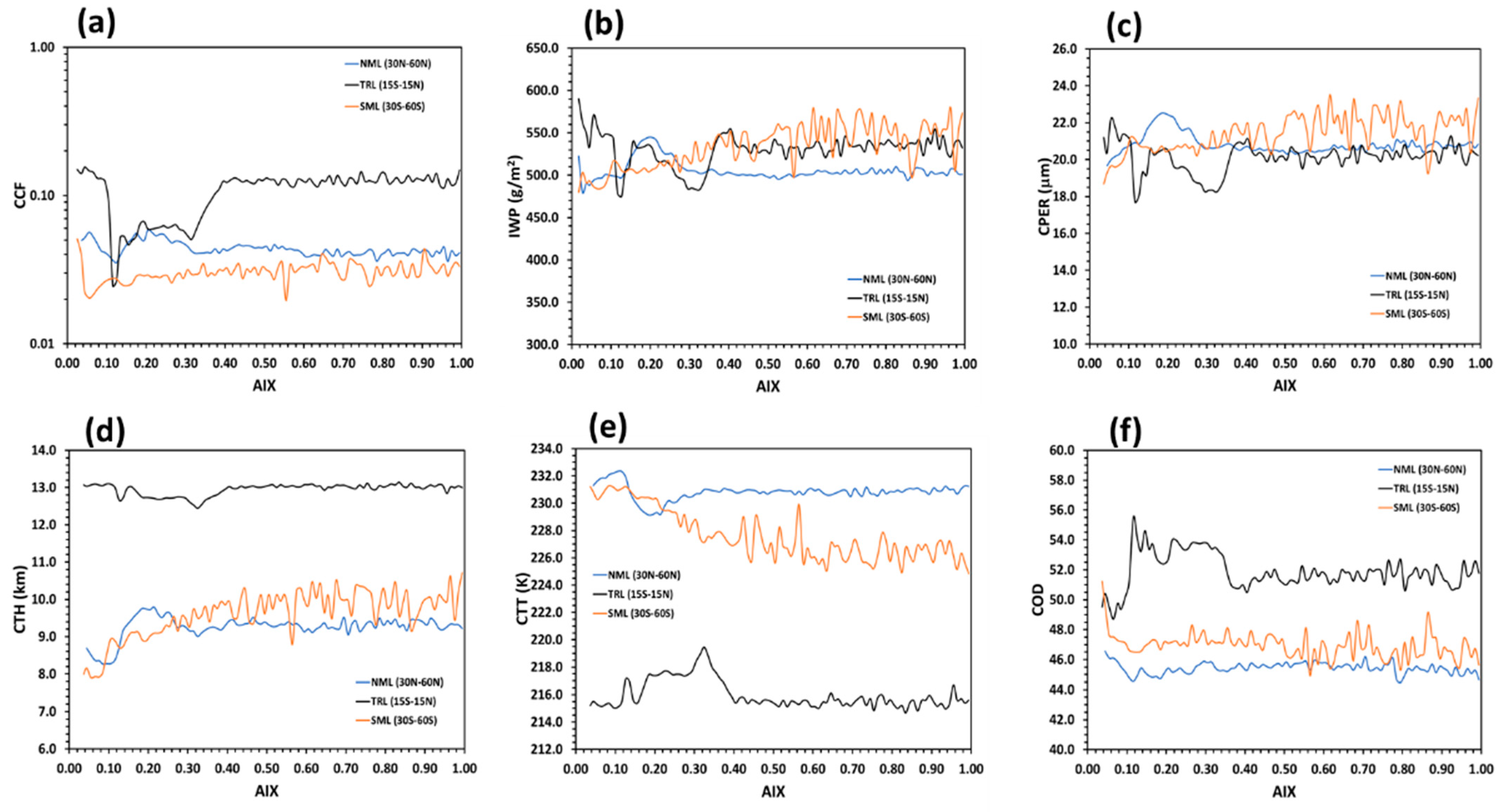
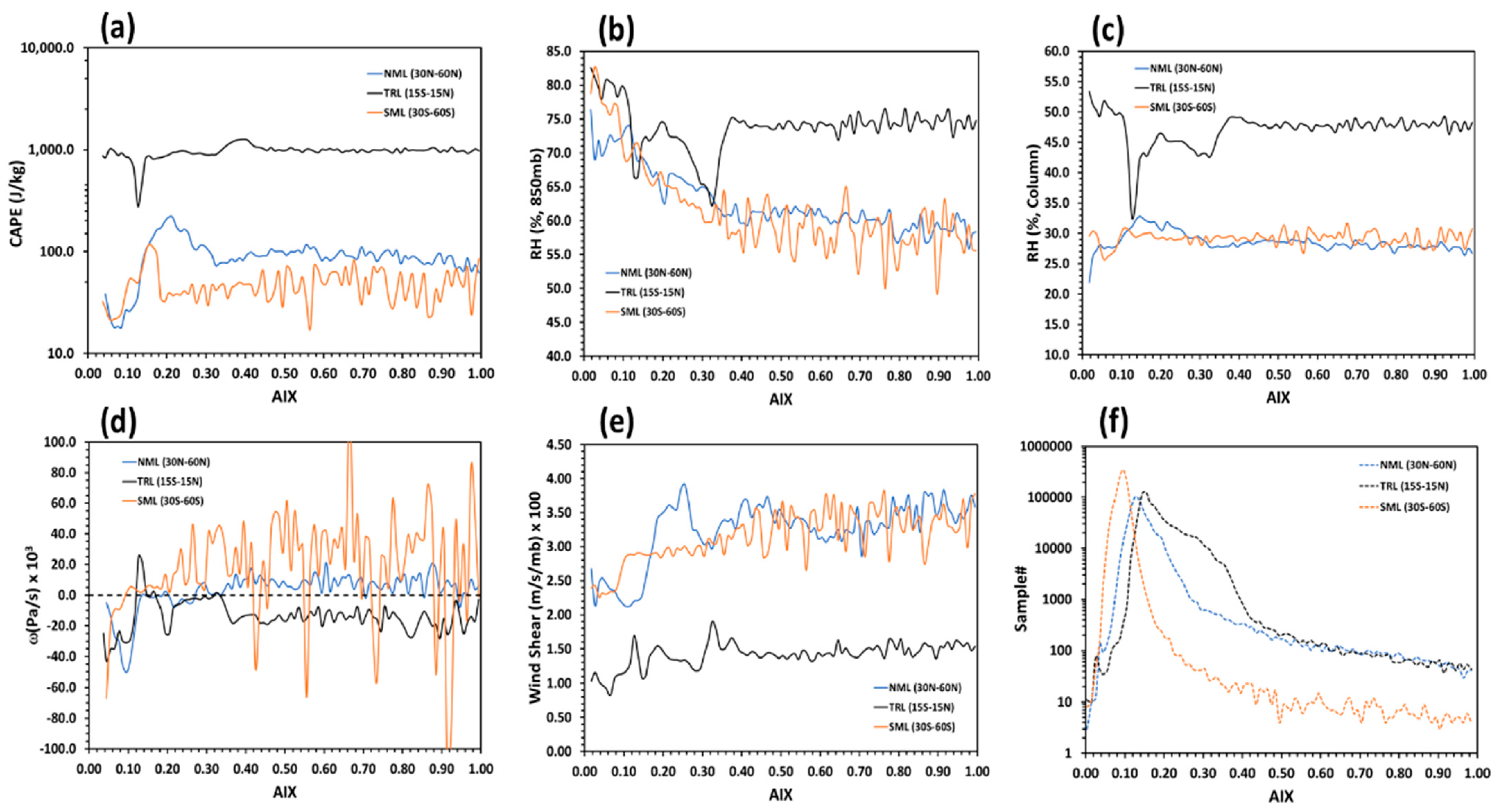
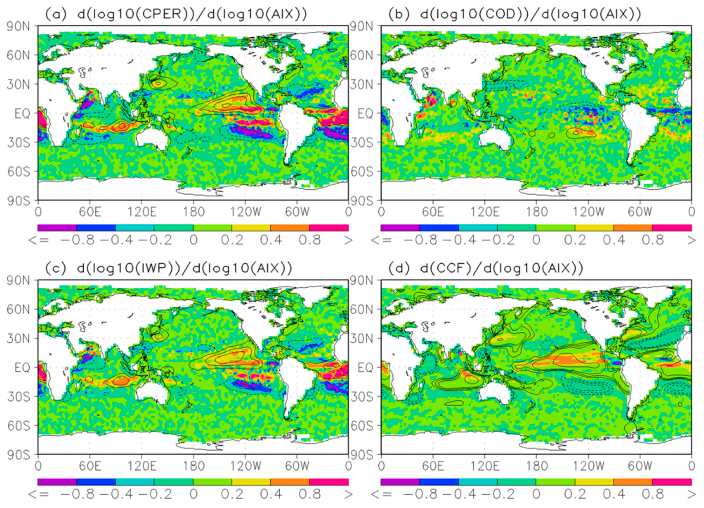
We first examined the global distribution of long-term averaged AIX and six cloud variables to identify regions with intensive DCCs and potential aerosol effect. The aerosol effect on DCCs is also simply called the aerosol indirect effect (AIE) of DCCs hereafter. Then, statistical relationships of cloud and meteorological variables with AIX were computed and examined to define the sensitive regime of AIX for the AIE. For the tropical latitude belt (named TRL hereafter) of 15° S–15° N, the northern middle latitude belt (NML) of 30° N–60° N, and the southern middle latitude belt (SML) of 30° S–60° S, where DCCs appear more frequently (see Section 4.1 below), we performed further investigation to determine if the variations of six cloud variables (CPER, IWP, COD, CCF, CTH, and CTT) in the AIE sensitive regime of AIX are mainly due to the AIE or the covariance of meteorological conditions. Specifically, we performed a multiple-variables linear regression (MVLR) for the individual six cloud variables with AIX and fourteen selected meteorological variables over five selected regions in TRL, NML, and SML. The five selected regions are listed in Table 1. The first region is over the northwest Pacific Ocean (named NWPO hereafter) in NML, the second region is over the tropical west Pacific Ocean (TWPO) in TRL, the third region is over the southern Indian Ocean (SIO) in SML. DCCs appear most frequently in these first three regions of NML, TRL, and SML, respectively (see Section 4.1 below), which is the reason they were selected in our study. The fourth region is over the coastal oceans of southeast China (named SEC) and the last region is over the middle subtropical Pacific Ocean (MSPO). SEC and MSPO were selected due to interesting distribution features of the cloud variables (see Section 4.1 below), which may contain the signatures of AIE as presented in the following Section 4.1.
Since aerosols may suppress or invigorate convective cloud development [8,9,10], we first selected AIX as one of the variables used in the MVLR analysis. The availability of surface CAPE, atmospheric moisture, and precipitable water along with the meteorological conditions near the cloud base are critical for the development of wet convection [8,9] so that CAPE, RHclm, PW, U850, V850, ω850, RH850, and T850 were selected from CFSR as the meteorological variables used in the MVLR. Moreover, meteorological condition in the subcloud layer (or near the surface), such as “cool pool”, can be important for the development of a DCC from shallow convection [8,14,48]. Thus, RH2m, T2m, U10m, V10m, and ωsig995 were also added to the list of meteorological variables used in our MVLR. Some previous studies, e.g., [49,50,51] also indicated that tropospheric vertical wind shear is critical in organizing mesoscale convective systems and determines whether aerosols suppress or enhance convective strength. Therefore, we also included VSHW as a variable in the MVLR analysis. The annual mean values of six cloud variables, AIX, and fourteen meteorological variables were selected and used for the MVLR as expressed in Equation (2):
C V i j ,   k = a 0 j , k + a 1 j , k x 1 , i j , k + a 2 j , k x 2 , i j , k + + a 15 j , k x 15 , i j , k
where CV and index i (= 1, 2, …, 6) represent one of the six cloud variables (CPER, IWP, COD, CCF, CTH, CTT). j (= 1, 2, …, 5) is one of the five regions (MSPO, NWPO, SEC, SIO, TWPO) listed in Table 1. The logarithm values of the six cloud variables were used in the MVLR to account for some of the nonlinearity in the linear regression. k is the index of year, which changes from 1 (1982) to 38 (2019). x1, x2, …, x15 are fifteen selected aerosol and meteorological variables (AIX, CAPE, PW, RHclm, RH850, RH2m, T850, T2m, U850, U10m, V850, V10m, ω850, ωsig995, VSHW). a0 is the constant term and a1, a2, …, a15 are fifteen linear regression parameters (or slopes).
At last, we tried to determine the sensitive (or active) regions of the aerosol effect on DCCs over the global oceans by investigating the sensitivity of a cloud variable relative to AIX defined as Δlog10(cloud-variable)/Δlog10(AIX). This sensitivity is actually the slope of the linear regression of a cloud variable relative to AIX [52]. The above correlation analysis suggests the three microphysical cloud variables (CPER, IWP, COD), especially CPER and IWP, are more sensitive to an AIX change than the three macrophysical cloud variables (CCF, CTH, CTT). Among the three macrophysical cloud variables, CCF has some sensitivity to an AIX change but CTH and CT show only weak sensitivity. Thus, we performed linear regression calculations for log10(cloud-variable) relative to log10(AIX) for CPER, IWP, COD, and CCF on a 2.5° × 2.5° spatial grid over the global oceans using their long-term averaged monthly mean values in 0.1° × 0.1° spatial resolution. Using the logarithm considers the nonlinearity aspect of the sensitivity computation based on the linear regression, and the results can be used effectively to diagnose and capture the signature of the aerosol effect on clouds [52,53].

4. Results

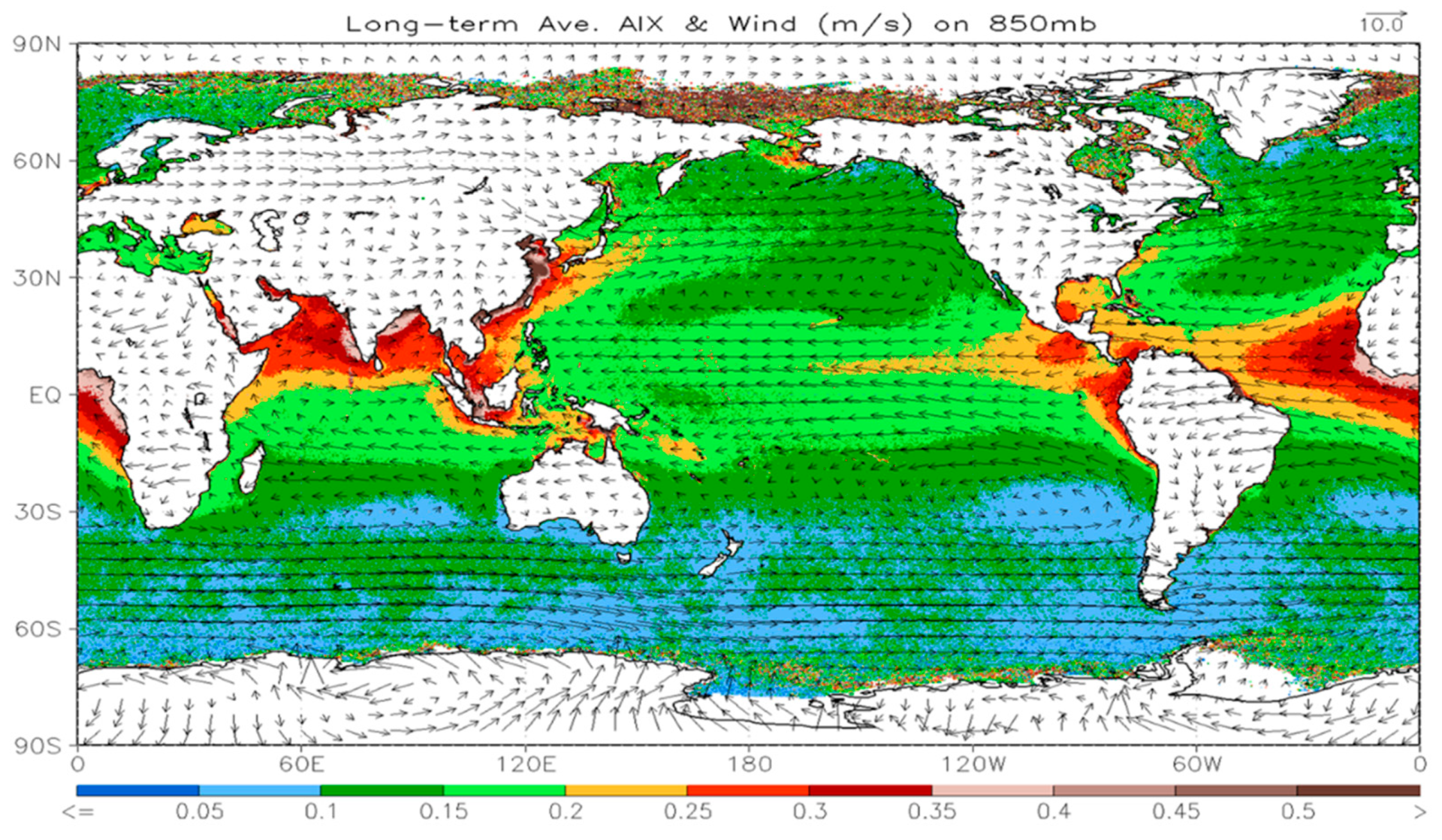
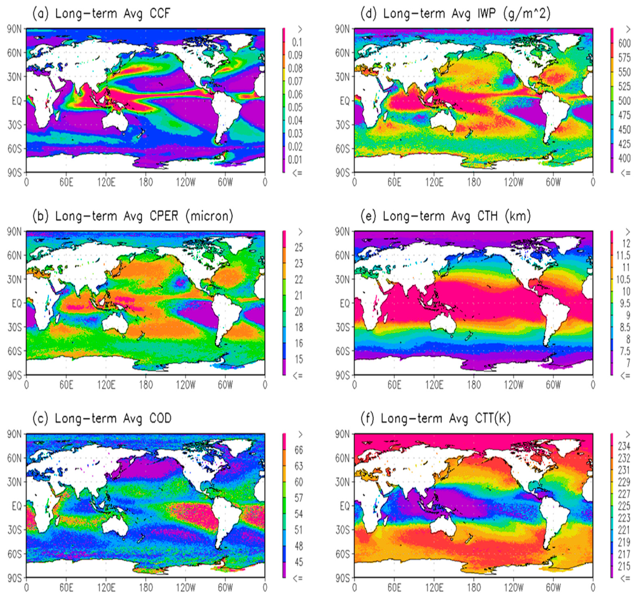
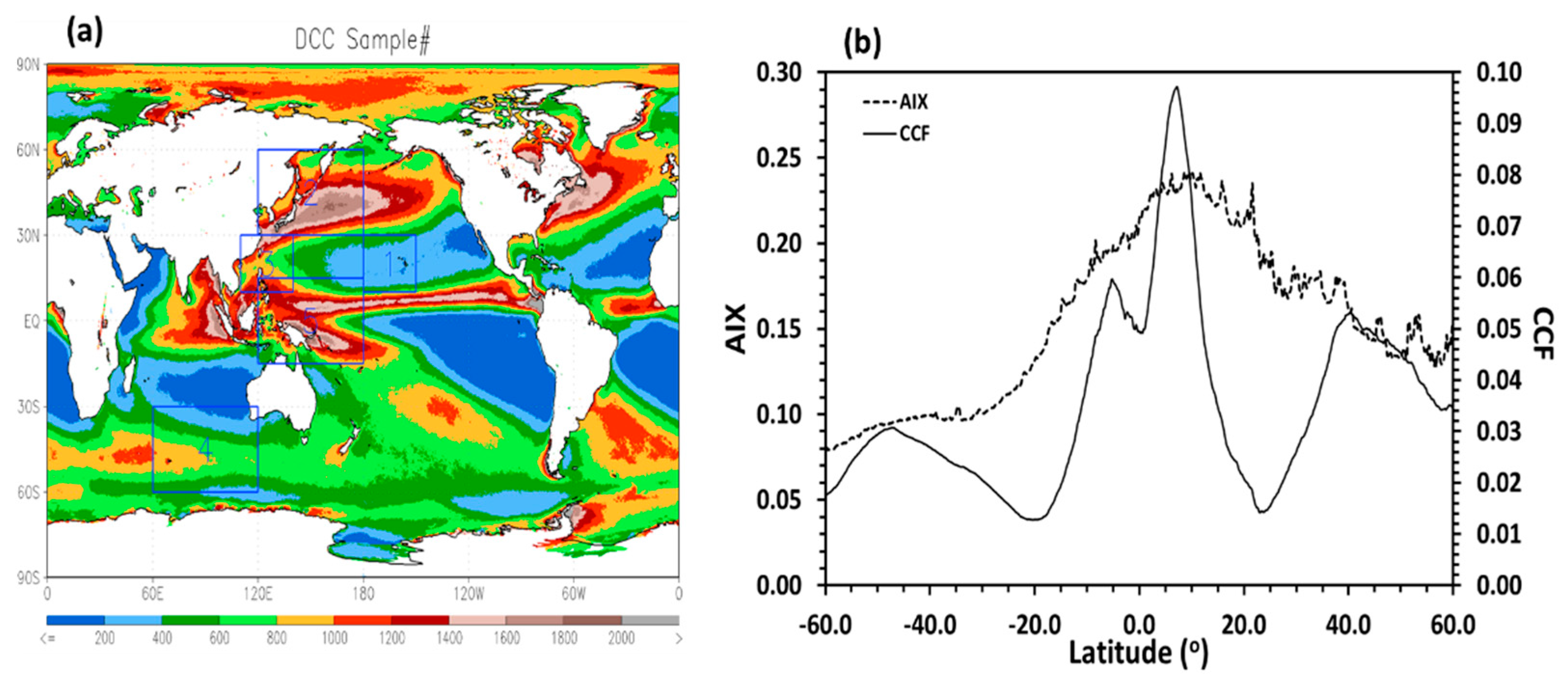
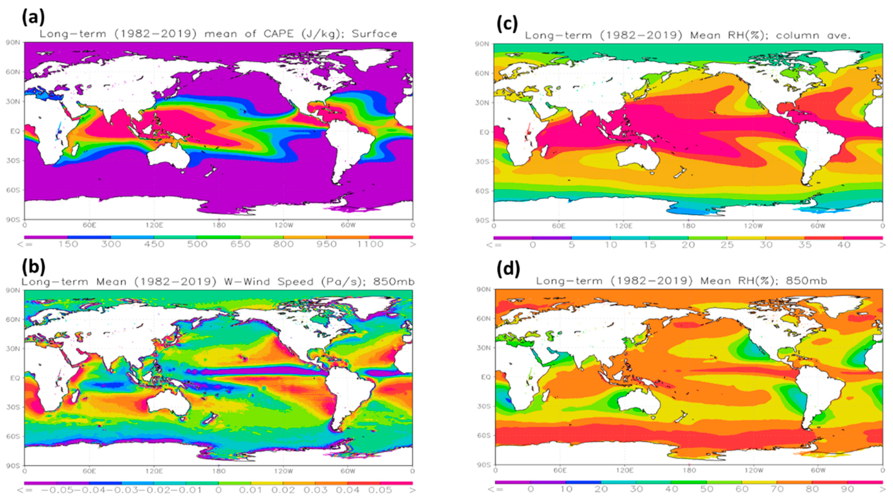
4.1. Global Long-Term Mean Distributions

Figure 1 shows the distribution of long-term (1982–2019) averaged monthly mean AIX over the global oceans, which is overlaid with long-term averaged horizontal wind vectors on 850 mb pressure level. It is seen that AIX values over coastal oceanic areas are generally higher than those over remote oceans due to abundant continental aerosols flowing out from their source regions over land. For example, these continental aerosols can be dust over the west coast of North Africa, biomass burning over the west coast of Central/South Africa, industrial pollution and dust particles over the Arabian Sea, the Bay of Bengal, and the coastal oceans of China, or industrial pollution and biomass burning over the Indonesia Seas. Many of these aerosols are hygroscopic and may be lifted into the cloud layer, especially in the development stage of DCCs, to become activated CCNs and INPs and modify cloud microphysical and macrophysical properties. AIX values are the highest in the tropical oceans, moderate over the oceans in the northern middle latitudes, and lowest over the southern oceans (see also Figure 3b). Thus, it is reasonable to speculate that the aerosol effect on DCCs could be more active in the northern hemisphere (NH) than in the southern hemisphere (SH) and most active in the tropics, which will be confirmed in our subsequent analyses.
Figure 2 shows the distributions of six cloud variables (CCF, CPER, COD, IWP, CTH, and CTT) of DCCs for their long-term averaged monthly mean values over the global oceans. Total DCC sample numbers used to compute the long-term averaged monthly mean values for the six cloud variables are displayed in Figure 3a, which can be considered as the frequence of DCC occurance. We can see relatively high CCF values are mainly located over the three zonal latitude belts (Figure 2a). The first is 30° N–60° N of northern middle latitudes (named NML), the second is 30° S–60° S of southern middle latitudes (SML), and the last is 15° S–15° N of tropical latitudes (TRL). CCF shows the highest value over the tropical convergence zones due to strong convection. There are also relatively high CCF values in the NML storm corridors over the Northern Pacific Ocean and the Northern Atlantic Ocean, where mesoscale convective cloud systems (MCS) are active. CCF values in the SML storm corridors over the Southern Indian Ocean and the Southern Atlantic Ocean are also somewhat high due to MCS convection. CCF values are relatively low in the subtropical latitudes of both hemispheres where atmospheric subsidence motions are prevailing. The CCF of NML is evidently higher than that of SML while CCF is the highest in TRL. This might be related to some extent to the relatively high aerosol loading in the NH compared to the SH and the highest aerosol loading over TRL in addition to the convections, which will be furtherly investigated in Section 4.4 below. The latitudinal distribution of AIX and CCF can be seen more clearly in Figure 3b, which shows the zonally averaged climatology of AIX and CCF, respectively.
Similar to CCF, three zonal latitude belts with relatively high CPER and IWP but relatively low COD are also observed for DCCs and their NH and SH differences are less distinct than CCF. COD is relatively high but CPER and IWP are relatively low in the subsidence regions over the subtropical latitudes of both hemispheres, except in the middle subtropical Pacific Ocean (named MSPO), where CPER and IWP become somewhat high. It is interesting to note (see Figure 2a–d) that there is a tongue extending from 110° E to 140° E between 10° N and 30° N with relatively low CPER and IWP but somewhat high CCF and COD over the coastal oceans of the southeast China (SEC), which is most prominent in winter season (not shown here). This might be the signature of aerosol microphysical invigoration effect (aerosols invigorate convection through ice processes) since offshore anthropogenic aerosol loading is prominent in this region [54,55,56], especially in the winter season [26,57], due to the transport of air pollution from mainland China. It is expected that precipitation should be enhanced accordingly in the same region due to invigorated convection, which was indeed observed in TRMM satellite rainfall measurements see [58,59], especially in the winter season (DJF). More analysis of AIE on DCCs in SEC will be performed in the following subsections.
The highest CTH and lowest CTT appear over the tropics and gradually decrease and increase, respectively, toward higher latitudes. This nearly zonal distribution of CTH and CTT is likely more related to atmospheric circulation and DCC dynamical and thermodynamic processes than to aerosol and cloud microphysical processes. In other words, the signature of aerosol effects on DCCs contained in CTH and CTT is likely obscured by DCC dynamical and thermodynamic processes and would subsequently be harder to observe in long-term averages (or climatology).
Figure 4 plots the distribution of long-term averaged monthly mean CAPE, ω850, RHclm, and RH850, respectively, over the global oceans. We can see the convective available potential energy (Figure 4a) is nearly in a zonal distribution with the highest values in the tropics, especially in the tropical convergence zones, and dissipates rapidly toward middle and high latitudes. Accordingly, upward motion (negative ω in Figure 4b) is most prominent in the tropical convergence zones and downward motion is mainly located in the subsidence areas over the subtropical latitudes of both hemispheres, especially over the west coastal oceans of the major continents. Weak upward motion is a general feature beyond 30° N and 45° S, respectively, except relatively high positive values (downward motion) in a narrow tongue region over the northeastern costal oceans of China and USA, and the broad areas of East Siberian Sea, Chukchi Sea, and Beaufort Sea in polar latitudes. The highest value of RHclm is in the tropics, especially in the tropical convergence zones, and decreases gradually toward high latitudes. RH850 shows similar features in the tropics as RHclm, except that the belt with the highest value is more concentrated in the convergence zones. Relatively low values appear in the subsidence areas of subtropical altitudes in both hemispheres (Figure 4d), especially over the west coastal oceans of the major continents. RH850 values are relatively high in the polar latitudes of both hemispheres, which is opposite to that of RHclm. The spatial distribution of RH850 seems more related to the three meridional atmospheric circulations than that of RHclm. The spatial features of these important aerosol, cloud, and meteorological fields will help us analyze the aerosol effect on DCCs in the subsequent study.

4.2. Statistical Features

Figure 5 shows statistical relationships of AIX with CCF, IWP, CPER, CTH, CTT, and COD for their long-term averaged values in the three latitudinal regions (NML, TRL, and SML) where DCCs appear more frequently than other latitudinal locations (see Figure 3a). The six cloud variables are binned according to AIX with 0.01 incremental interval and the mean values for individual bins are computed and displayed for the three regions. The numbers of the sample size for individual bins are displayed later in Figure 6f. In the TRL, large variations of the six cloud variables are mainly observed between 0.1 and 0.4 of AIX and they stay relatively stable outside of this range, which suggests this is the range of AIX values where the signature of aerosol effects on DCCs might manifest. Most of the sample numbers also fall in this range (named sensitive regime hereafter). At the same time, the variations may be also associated with the covariance of meteorological conditions. For example, the sudden drops (climbs) of CCF, CPER, IWP, and CTH (CTT and COD) at about 0.12 and 0.34 of AIX are associated clearly with low values of CAPE, RHclm, and RH850, high value of VSHW, and downward motion (or positive ω850) (see Figure 6). Similar drops are also noticed for RHclm, RH850, VSHW, and ω850, but not for CAPE at AIX~0.34. The variations of RHclm and RH850 with AIX increase are similar, which implies that convection is sufficiently strong in the atmospheric column that moisture is brought rapidly from ocean surface to the cloud layer. Thus, AIE signatures contained within the averaged six cloud variables between 0.1 and 0.4 of AIX in TRL may be masked by the covariance of meteorological conditions controlled by the atmospheric dynamical and thermodynamic processes of DCCs. Therefore, there is a need to separate the AIE and the covariance of meteorological conditions, which will be addressed in the subsequent correlation analysis.
For the NML, large variations of the six cloud variables are mainly observed between 0.1 and 0.32 of AIX and most of the sample numbers also fall in this regime. Thus, the range of AIX from 0.1 to 0.32 is the potential regime (or sensitive regime) where the aerosol effect on DCCs might manifest. In this regime, CCF, CPER, IWP, and CTH are relatively high, CTT is relativly low, and COD is relatively flat, in contrast generally to the TRL. A relativly high value is also observed in this regime for CAPE, RH850, and VSHW but not for ω850 and RHclm. Actually, different variations of RHclm and RH850, nearly zero vertical motion on 850 mb pressure level (ω850~0.0), and relatively strong wind shear in the sensitive regime suggest the convection in the NML is not as vigorous as in the TRL. The relatively high values of CCF, CPER, IWP, and CTH and relatively low values of CTT and COD may also contain an AIE signature in the sensitive regime. In other word, the signal of aerosol effects on DCCs may manifest in the long-term mean of the cloud variables in the NML, which will be further explored below. For the SML, there is a small increasing tendency in CCF, CPER, IWP, and CTH along with a small decreasing tendency in CTT and COD when AIX increases from 0.05 to 0.3 (sensitive regime). Relatively large fluctuations are noticed below 0.05 and above 0.3 of AIX (especially for AIX > 0.4), which is actually due to small sample size (see Figure 6f). The variations of CAPE, RH850, RHclm, and ω850 in the sensitive regime are similar to that in the NML (except the wind shear) but with much reduced magnitude. Different variations of RHclm and RH850 are also observed as in NML. Persistent upward motion is observed only at the beginning of the regime and turning to downward motion with evident fluctuation thereafter. Large positive and negative oscillations of ω850 are clear seen for AIX > 0.4. The nearly steady fluctuations of cloud and meteorological variables for the AIX larger than 0.4 are actually due to small sample size (see Figure 6f). Thus, similar to NML, the signature of aerosol effects on DCCs may manifest in the long-term mean of the cloud variables in the sensitive regime of SML but with much reduced signal due to obscuration by the covariance of meteorological conditions (see a further study below).

4.3. Correlation Analysis Result

Using the above Equation (2), we computed the correlation of the six cloud variables with AIX and the fourteen meteorological variables (CAPE, PW, RHclm, RH850, RH2m, T850, T2m, U850, U10m, V850, V10m, ω850, ωsig995, VSHW) that have a potential influence on DCCs in the five regions listed in Table 1. As an example, Table 2 and Table 3 list the individual linear correlation coefficients (Ci, i = 1, 2, …, 15) for AIX and the fourteen meteorological variables and the total multiple linear correlation coefficient (Ct) obtained from the multiple-variables linear regression for the cloud microphysical variables CPER and IWP, respectively, in the five regions. These correlation coefficients are normalized to 100 and expressed in the unit of percentage (%). The correlation coefficients in Table 2 and Table 3 for CPEF and IWP are also presented in Figure 7 along with the correlation coefficients for the other four cloud variables (COD, CCF, CTH, and CTT).
For the microphysical cloud variable CPER and IWP, their total multiple linear correlation (Ct) is generally above 80% in the five regions. AIX has the highest positive correlation with CPER and IWP among the fifteen variables, except in SIO. This suggests the aerosol effect on CPER and IWP of DCCs is likely to manifest in the long-term averaged satellite observations of clouds, especially in MSPO, TWPO, and NWPO where the correlation coefficient with AIX (C1) is above 60%. As a result, CPER and IWP may be increased (decreased) due to an increase (decrease) of aerosol loading. This also supports our previous speculation that relatively high (or low) CPER and IWP in Figure 2b,d in MSPO (or SEC) may be a manifestation of AIE. There is also a relatively high correlation (C4 or C5) with the relative humidity (RHclm or RH850) so that they are also important to some extent for the change of CPER and IWP but insufficient to conceal the aerosol effect. Vertical motion in the cloud base (ω850) or subcloud layer (ωsig995) shows the highest negative correlation (C13 or C14), except in SIO, which suggests the vertical motion may also contribute somewhat to the change of CPER and IWP in MSPO, NWPO, SEC, and TWPO. The highest negative correlation of IWP with AIX and low positive correlation of CPEF with AIX in SIO suggest AIE signature may manifest in the change of IWP rather than in that of CPEF in SIO, where aerosols over the remote southern oceans are relatively less abundant (see Figure 1). The correlation of cloud microphysical variable COD with AIX is not prominent and comparable to the correlation of COD with the relative humidity or the vertical motion (see Figure 7c), only becomes somewhat prominent in MSPO and TWPO but the absolute value of the correlation coefficient C1 is still less than 50%. Thus, AIE signatures contained in COD variations may concealed by the covariance of meteorological conditions.
For the macrophysical cloud variable CCF (Figure 7d), its correlation with AIX is small, except in SIO where the negative correlation is close to 70% and is the highest in the absolute value among the fifteen correlation coefficients. Therefore, DCC suppression or invigoration due to the change of aerosol loading is likely to manifest in CCF of SIO but not in the other four regions, where the covariance of meteorological conditions may easily conceal the aerosol effect on CCF. For the macrophysical cloud variable CTH (Figure 7e), its correlation with AIX is not prominent, except in TWPO where the positive correlation is about 56% and is the highest in the absolute value among the fifteen correlation coefficients. Thus, DCC suppression or invigoration may manifest in CTH in TWPO but hardly to manifest in the other four regions, where the covariance of meteorological conditions may play a more important role than the aerosol effect on CTH. For the macrophysical cloud variable CTT (Figure 7f), its correlation with AIX (C1) is inconspicuous compared to some of the meteorological variables, such as C15 (VSHW) for MSPO, C14sig995) for NWPO, C8 (T2m) for SEC, C7 (T850) for SIO, and C11 (V850) for TWPO, so that the signature of aerosol effect on CTT can be easily obscured by the covariance of meteorological conditions and becomes almost impossible to manifest.

4.4. AIE Active Regions

In order to determine the active regions of the aerosol effects on DCCs over the global oceans, the sensitivity of cloud variables of CPER, COD, IWP, and CCF relative to AIX defined as Δlog10(cloud-variable)/Δlog10(AIX) is displayed over the global oceans in Figure 8. The confidence level of the positive and negative sensitivity above 95% is also displayed by the solid and dash contours, respectively. We can see in Figure 8a that there is generally a high positive sensitivity of CPER to AIX changes in the tropical convergence zones with strong convections and a high negative sensitivity of CPER to AIX changes in the subtropical subsidence regions. This suggests an increase of aerosol loading tends to increase DCC particle size in the tropical convergence zones but decrease it in the subtropical subsidence regions. It is notable that there is a high positive sensitive region in the central and eastern subtropical Pacific Ocean and the northwestern Pacific Ocean. MSPO and NWPO listed in Table 1 fall into these two sensitive regions, respectively. This sensitivity study and the above correlation analysis suggest the aerosol effects on DCCs are likely to manifest in the long-term averaged satellite observed CPER of DCCs in these regions. The sensitivity of IWP to AIX change in Figure 8c is very similar to that of CPER, which is also consistent with the result of the above correlation analysis. COD also shows similar sensitivity features as CPER and IWP but with reversed positive and negative phases and weaker signals (see Figure 8b). Thus, cloud dynamical and thermodynamic processes may easily obscure the aerosol effect on COD and make it hard to manifest. CCF also displays similar but somewhat less distinctive features in the sensitivity compared to CPER and IWP (Figure 8d), which suggests that the aerosol effect on the microphysical cloud variables may furtherly propagate to CCF. To confirm this speculation, the sensitivity of CCF to the AIX variation is decomposed into two terms in the following Equation (3):
δ ( C C F ) δ ( l o g 10 ( A I X ) ) = δ ( C C F ) δ ( l o g 10 ( C P E R ) ) × δ ( l o g 10 ( C P E R ) ) δ ( l o g 10 ( A I X ) ) + r e s i d u a l .
Since CPER is more susceptible to AIX variations than CCF, the first term on the right-hand side of Equation (3) contains the CCF change mainly due to CPER variation as a result of aerosol-cloud interaction. The residual term contains the CCF change mainly due to other effects, such as meteorological covariations, detection errors, etc. The term on the left-hand side and the first term on the right-hand side (along with its two components) are shown in Figure 9 for long-term averaged CCF, CPER, and AIX. The regions with significant positive and negative sensitivities of CCF to AIX variations clearly seen in Figure 9b (left-hand term of Equation (3)) also show generally a significant positive sensitivity of CCF to CPER variations in Figure 9c, which confirms the aerosol effect on CPER may propagate furtherly to CCF. Comparing Figure 9b (left-hand term) and Figure 9d (the first term on the right-hand side of Equation (3)), their distribution patterns are very similar except in some narrow or small regions in yellow/red and blue/purple colors over the tropical convergence zones in Figure 9b, where the very high positive or negative sensitivities in Figure 9b disappear in Figure 9d. This suggests, in addition to the aerosol effect, the other effects (such as meteorological covariations) contained in the residual term may contribute to the CCF change significantly in these narrow or small tropical regions and conceal the aerosol effect on CCF. Thus, the macrophyical cloud variable CCF is less susceptible to AIX changes than the microphysical cloud variables CPER and IWP in the tropical regions with strong convections, which is consistent with the result of the above correlation analysis.

5. Discussion

Since the climate of the atmosphere represents the mean state of the atmosphere for a given relatively long time period, it is important to detect the signatures of aerosol-cloud interaction in long-term averaged satellite observations. This is our major motivation for performing the current study of aerosol effects on DCCs with respect to the long-term mean values of aerosol and cloud variables from satellite observations. Monthly and annual mean values of aerosol and cloud variables from satellite observations have fewer spatial gaps over the globe and less noise compared to their instantaneous or short-term averaged counterparts. Thus, they are more useful for identifying sensitive regimes (or ranges) of aerosol loading and the active geolocations of aerosol effects on DCCs over the global oceans from a climatology perspective. Even though our statistical correlation and regression analyses on long-term averaged aerosol and cloud variables from satellite observations are useful for detecting some signatures of aerosol effects on DCCs over the global oceans, it is important to address some possible limitations of our study.
Previous studies, e.g., [12,21] indicated, in addition to aerosol amount and size, aerosol type is also an important factor in determining the aerosol effects on convective clouds, especially the either suppression or invigoration of DCCs. There is only one aerosol variable AIX available in the long-term satellite observation for us to use in the current study so that the aerosol type effect on DCCs is missing in our analysis, which may partially explain the weak sensitivity of the aerosol effect on CTH and CTT of DCCs in our analyses. Aerosol effects on DCCs are much more complex and nonlinear, but our statistical analyses are mainly based on linear analyzing techniques, even though the logarithmic values of some cloud variables are used to remedy this deficiency. The relatively low values (<80%) of multiple linear correlation coefficients for CTH and CTT still remain in some regions with more intensive DCCs, which is likely due to this deficiency, and nonlinear analyzing techniques should be explored in the future for further improvement on our analyses.
There are also artifacts or uncertainties in the satellite observations of aerosols and DCCs (uncertainties caused by the assumptions of aerosol optical properties, scattering properties of ice crystals, vertical distribution of ice crystals, filtering criteria for selecting DCCs, etc.). These uncertainties may result in inconsistent features in our statistical correlation analysis for aerosol and cloud variables, such as the incoherent changing tendency among cloud variables with AIX increasing when sample size is not sufficiently large. Thus, identifying coherent informative features is critical in the detection of an AIE signature in our statistical correlation analysis. The observational uncertainties may also smear the sensitivity of cloud variables relative to the AIX change in the detection of AIE active regions based on our linear regression analysis. Thus, the significance of sensitivity in our regression analysis, along with the coherent correlation features between aerosol and cloud variables in the spatial distributions, are critical for identifying the signature of AIE in our study. Therefore, our identification of sensitive AIX regimes and active geolocations of AIE for DCCs is more of a first order quantitative analysis. Further in-depth quantitative analysis of various processes involved in the AIE for different types of aerosols and different regions of DCCs and their global climate implications are needed in future studies based on combined multiple observations (satellite, airborne, and in situ) and model (box, regional, and global) simulations.

6. Summary and Conclusions

Long-term (1982–2019) satellite observations of aerosols and clouds, along with CFSR reanalysis, have been used to study the aerosol effects on DCCs over the global oceans from a climatological perspective. Our focus is on exploring and identifying sensitive aerosol regimes and active geolocations of the aerosol effects on DCCs by using statistical techniques, such as correlation analysis and multiple-variables linear regression.
We found the aerosol effects tend to manifest more easily on the long-term mean values of observed cloud microphysical variables (CPER, IWP, and COD) than on observed cloud macrophysical variables (CCF, CTH, and CTT). Among the three observed cloud microphysical variables, CPER and IWP are more susceptible to the aerosol effect than COD from a climatological perspective. An increase of aerosol loading tends to increase DCC particle size and IWP in the tropical convergence zones but decrease them in the subtropical subsidence regions. An increase of aerosol loading may also decrease COD in the tropical convergence zones and increase COD in the subtropical subsidence regions, but it can be easily concealed by cloud dynamical and thermodynamic processes and make it hard to be detected in COD variation. The aerosol effect on CPER and IWP of DCCs is also likely to manifest over the northwestern Pacific Ocean and central and eastern subtropical Pacific Ocean in the long-term averaged satellite observations.
Among the three observed cloud macrophysical variables, CCF is somewhat more susceptible to the aerosol effect than CTH and CTT since they are mainly influenced by cloud dynamical and thermodynamic processes. Accordingly, the aerosol effect on the microphysical cloud variables may further propagate to CCF rather than to CTH and CTT in the long-term averaged satellite observations. In consideration of large AIE uncertainties for DCCs in current global climate models, the results of this study based on long-term averaged satellite observations are valuable for the evaluation and improvement of the aerosol-cloud interaction in these models.

Author Contributions

Conceptualization, X.Z.; methodology, X.Z.; formal analysis, X.Z. and M.J.F.; writing—original draft preparation, X.Z.; writing—review and editing, X.Z. and M.J.F. All authors have read and agreed to the published version of the manuscript.

Funding

This research was funded by NOAA/NESDIS/NCEI Climate Data Record (CDR) program and X.Z. was also funded by NCEI base fund.

Data Availability Statement

The data sources used in this study have been provided in Section 2 with the data weblinks. For the data produced in this study, please email to the lead author.

Acknowledgments

The authors (X.Z. and M.J.F.) would like to acknowledge the support from the CDR program at the National Centers for Environmental Information (NCEI) of NOAA/NESDIS. We also would like to acknowledge two anonymous reviewers’ comments and suggestions, which is helpful for the improvement of the paper. NCEI internal review provided by Saha Korak, Anand Inamdar, and Yongsheng Zhang is greatly appreciated. The views, opinions, and findings contained in this paper are those of the author(s) and should not be construed as an official National Oceanic and Atmospheric Administration or U.S. government position, policy, or decision.

Conflicts of Interest

The authors declare no conflict of interest.

Abbreviations

ACIaerosol cloud interaction
AIEaerosol indirect effect
AIXaerosol index
AOTaerosol optical thickness
AVHRRAdvanced Very High-Resolution Radiometer
CAPEconvective available potential energy
CCNcloud condensation nuclei
CDR(s)climate data record(s)
CFSRclimate forecast system reanalysis
CODcloud optical depth
CPERcloud particle effective radius
CTHcloud top height
CTTcloud top temperature
DCC(s)deep convective cloud(s)
EUMETSATEuropean Organization for the Exploitation of Meteorological Satellites
GACglobal area coverage
HIRSHigh-resolution Infra-Red Sounder
INP(s)ice nucleating particle(s)
IWPice water path
NASANational Aeronautics and Space Administration
MCSmesoscale convective cloud systems
MetOpMeteorological Operational Satellites
MODISModerate-resolution Imaging Spectroradiometer
MVLRmultiple-variables linear regression
NCEINational Centers for Environmental Information
NCEPNational Centers for Environmental Prediction
NESDIS National Environmental Satellite, Data, and Information Service
NHnorthern hemisphere
NMLnorthern middle latitudes
NOAA National Oceanic and Atmospheric Administration
PATMOS-x Pathfinder Atmospheres-Extended
RH relative humidity
SHsouthern hemisphere
SMLsouthern middle latitudes
STAR Center for Satellite Applications and Research
TRLtropical latitude

References

  1. Mason, B.J. The Physics of Clouds; Oxford: Oxford, UK, 2010. [Google Scholar]
  2. Pruppacher, H.R.; Klett, J.D. Microphysics of Clouds and Precipitation; Kluwer Academy: Dordrecht, The Netherlands, 1997; p. 954. [Google Scholar]
  3. Arakawa, A. The cumulus parameterization problem: Past, present, and future. J. Clim. 2004, 17, 2493–2525. [Google Scholar] [CrossRef]
  4. Futyan, J.M.; Del Genio, A.D. Deep convective system evolution over africa and the tropical atlantic. J. Clim. 2007, 20, 5041–5060. [Google Scholar] [CrossRef]
  5. Khain, A.; Rosenfeld, D.; Pokrovsky, A. Aerosol impact on the dynamics and microphysics of deep convective clouds. Q. J. Roy. Meteor. Soc. 2005, 131, 2639–2663. [Google Scholar] [CrossRef] [Green Version]
  6. Lohmann, U.; Feichter, J. Global indirect aerosol effects: A review. Atmos. Chem. Phys. 2005, 5, 715–737. [Google Scholar] [CrossRef] [Green Version]
  7. Stevens, B.; Feingold, G. Untangling aerosol effects on clouds and precipitation in a buffered system. Nature 2009, 461, 607–613. [Google Scholar] [CrossRef]
  8. Tao, W.K.; Chen, J.P.; Li, Z.Q.; Wang, C.; Zhang, C.D. Impact of aerosols on convective clouds and precipitation. Rev. Geophys. 2012, 50, 1–62. [Google Scholar] [CrossRef] [Green Version]
  9. Fan, J.W.; Wang, Y.; Rosenfeld, D.; Liu, X.H. Review of aerosol-cloud interactions: Mechanisms, significance, and challenges. J. Atmos. Sci. 2016, 73, 4221–4252. [Google Scholar] [CrossRef]
  10. Seinfeld, J.H.; Bretherton, C.; Carslaw, K.S.; Coe, H.; DeMott, P.J.; Dunlea, E.J.; Feingold, G.; Ghan, S.; Guenther, A.B.; Kahn, R.; et al. Improving our fundamental understanding of the role of aerosol-cloud interactions in the climate system. Proc. Natl. Acad. Sci. USA 2016, 113, 5781–5790. [Google Scholar] [CrossRef] [Green Version]
  11. Li, Z.Q.; Rosenfeld, D.; Fan, J.W. Aerosols and their impact on radiation, clouds, precipitation, and severe weather events. In Oxford Research Encyclopedia of Environmental Science; Oxford University Press USA: New York, NY, USA, 2017; pp. 1–36. [Google Scholar]
  12. Rosenfeld, D.; Lohmann, U.; Raga, G.B.; O’Dowd, C.D.; Kulmala, M.; Fuzzi, S.; Reissell, A.; Andreae, M.O. Flood or drought: How do aerosols affect precipitation? Science 2008, 321, 1309–1313. [Google Scholar] [CrossRef] [Green Version]
  13. Igel, A.L.; van den Heever, S.C. Invigoration or enervation of convective clouds by aerosols? Geophys. Res. Lett. 2021, 48, e2021GL093804. [Google Scholar] [CrossRef]
  14. Li, X.W.; Tao, W.K.; Masunaga, H.; Gu, G.J.; Zeng, X.P. Aerosol effects on cumulus congestus population over the tropical pacific: A cloud-resolving modeling study. J. Meteorol. Soc. Jpn. 2013, 91, 817–833. [Google Scholar] [CrossRef] [Green Version]
  15. Andreae, M.O.; Rosenfeld, D.; Artaxo, P.; Costa, A.A.; Frank, G.P.; Longo, K.M.; Silva-Dias, M.A.F. Smoking rain clouds over the amazon. Science 2004, 303, 1337–1342. [Google Scholar] [CrossRef] [PubMed] [Green Version]
  16. Koren, I.; Feingold, G.; Remer, L.A. The invigoration of deep convective clouds over the atlantic: Aerosol effect, meteorology or retrieval artifact? Atmos. Chem. Phys. 2010, 10, 8855–8872. [Google Scholar] [CrossRef] [Green Version]
  17. Li, Z.Q.; Niu, F.; Fan, J.W.; Liu, Y.G.; Rosenfeld, D.; Ding, Y.N. Long-term impacts of aerosols on the vertical development of clouds and precipitation. Nat. Geosci. 2011, 4, 888–894. [Google Scholar] [CrossRef]
  18. Niu, F.; Li, Z.Q. Systematic variations of cloud top temperature and precipitation rate with aerosols over the global tropics. Atmos. Chem. Phys. 2012, 12, 8491–8498. [Google Scholar] [CrossRef] [Green Version]
  19. Fan, J.W.; Leung, L.R.; Rosenfeld, D.; Chen, Q.; Li, Z.Q.; Zhang, J.Q.; Yan, H.R. Microphysical effects determine macrophysical response for aerosol impacts on deep convective clouds. Proc. Natl. Acad. Sci. USA 2013, 110, E4581–E4590. [Google Scholar] [CrossRef] [Green Version]
  20. Fan, J.W.; Rosenfeld, D.; Zhang, Y.W.; Giangrande, S.E.; Li, Z.Q.; Machado, L.A.T.; Martin, S.T.; Yang, Y.; Wang, J.; Artaxo, P.; et al. Substantial convection and precipitation enhancements by ultrafine aerosol particles. Science 2018, 359, 411–418. [Google Scholar] [CrossRef] [Green Version]
  21. Jiang, J.H.; Su, H.; Huang, L.; Wang, Y.; Massie, S.; Zhao, B.; Omar, A.; Wang, Z.E. Contrasting effects on deep convective clouds by different types of aerosols. Nat. Commun. 2018, 9, 3874. [Google Scholar] [CrossRef] [Green Version]
  22. Grabowski, W.W.; Morrison, H. Do ultrafine cloud condensation nuclei invigorate deep convection? J. Atmos. Sci. 2020, 77, 2567–2583. [Google Scholar] [CrossRef]
  23. Wang, Y.; Khalizov, A.; Levy, M.; Zhang, R.Y. New directions: Light absorbing aerosols and their atmospheric impacts. Atmos. Environ. 2013, 81, 713–715. [Google Scholar] [CrossRef]
  24. Wang, Y.; Vogel, J.M.; Lin, Y.; Pan, B.W.; Hu, J.X.; Liu, Y.G.; Dong, X.Q.; Jiang, J.H.; Yung, Y.L.; Zhang, R.Y. Aerosol microphysical and radiative effects on continental cloud ensembles. Adv. Atmos. Sci. 2018, 35, 234–247. [Google Scholar] [CrossRef]
  25. Bollasina, M.A.; Ming, Y.; Ramaswamy, V. Anthropogenic aerosols and the weakening of the south asian summer monsoon. Science 2011, 334, 502–505. [Google Scholar] [CrossRef] [Green Version]
  26. Li, Z.; Lau, W.K.-M.; Ramanathan, V.; Wu, G.; Ding, Y.; Manoj, M.G.; Liu, J.; Qian, Y.; Li, J.; Zhou, T.; et al. Aerosol and monsoon climate interactions over Asia. Rev. Geophys. 2016, 54, 866–929. [Google Scholar] [CrossRef]
  27. Wu, G.X.; Li, Z.Q.; Fu, C.B.; Zhang, X.Y.; Zhang, R.Y.; Zhang, R.H.; Zhou, T.J.; Li, J.P.; Li, J.D.; Zhou, D.G.; et al. Advances in studying interactions between aerosols and monsoon in China. Sci. China Earth Sci. 2016, 59, 1–16. [Google Scholar] [CrossRef]
  28. Li, R.; Dong, X.; Guo, J.C.; Fu, Y.F.; Zhao, C.; Wang, Y.; Min, Q.L. The implications of dust ice nuclei effect on cloud top temperature in a complex mesoscale convective system. Sci. Rep. 2017, 7, 13826. [Google Scholar] [CrossRef] [Green Version]
  29. Heidinger, A.K.; Foster, M.J.; Walther, A.; Zhao, X.P. The pathfinder atmospheres-extended avhrr climate dataset. Bull. Am. Meteorol. Soc. 2014, 95, 909–922. [Google Scholar] [CrossRef]
  30. Foster, M.J.; Phillips, C.; Heidinger, A.K.; Borbas, E.E.; Li, Y.; Menzel, W.P.; Walther, A.; Weisz, E. Patmos-x version 6.0: 40 years of merged avhrr and hirs global cloud data. J. Clim. 2022; in press. [Google Scholar]
  31. Heidinger, A.K.; Straka, W.C.; Molling, C.C.; Sullivan, J.T.; Wu, X.Q. Deriving an inter-sensor consistent calibration for the avhrr solar reflectance data record. Int. J. Remote Sens. 2010, 31, 6493–6517. [Google Scholar] [CrossRef]
  32. Heidinger, A.K.; Evan, A.T.; Foster, M.J. A naive bayesian cloud-detection scheme derived from calipso and applied withing patmos-x. J. Appl. Meteorol. Clim. 2012, 51, 1129–1144. [Google Scholar] [CrossRef]
  33. Walther, A.; Heidinger, A.K. Implementation of the daytime cloud optical and microphysical properties algorithm (dcomp) in patmos-x. J. Appl. Meteorol. Clim. 2012, 51, 1371–1390. [Google Scholar] [CrossRef]
  34. Heidinger, A.K.; Cao, C.; Sullivan, J.T. Using moderate resolution imaging spectrometer (modis) to calibrate advanced very high resolution radiometer reflectance channels. J. Geophys. Res. 2002, 107, 4702. [Google Scholar] [CrossRef]
  35. Cao, C.; Weinreb, M.; Xu, H. Predicting simultaneous nadir overpasses among polar-orbiting meteorological satellites for the intersatellite calibration of radiometers. J. Atmos. Ocean. Technol. 2004, 21, 537–542. [Google Scholar] [CrossRef]
  36. Cao, C.Y.; Xiong, X.X.; Wu, A.H.; Wu, X.Q. Assessing the consistency of avhrr and modis l1b reflectance for generating fundamental climate data records. J. Geophys. Res. Atmos. 2008, 113, D9. [Google Scholar] [CrossRef] [Green Version]
  37. Pavolonis, M.J.; Heidinger, A.K.; Uttal, T. Daytime global cloud typing from avhrr and viirs: Algorithm description, validation, and comparisons. J. Appl. Meteorol. 2005, 44, 804–826. [Google Scholar] [CrossRef]
  38. Rossow, W.B.; Schiffer, R.A. Advances in understanding clouds from isccp. Bull. Am. Meteorol. Soc. 1999, 80, 2261–2287. [Google Scholar] [CrossRef]
  39. Kubar, T.L.; Hartmann, D.L.; Wood, R. Radiative and convective driving of tropical high clouds. J. Clim. 2007, 20, 5510–5526. [Google Scholar] [CrossRef]
  40. Yuan, T.L.; Li, Z.Q. General macro- and microphysical properties of deep convective clouds as observed by modis. J. Clim. 2010, 23, 3457–3473. [Google Scholar] [CrossRef] [Green Version]
  41. Yuan, T.E.; Martins, J.V.; Li, Z.Q.; Remer, L.A. Estimating glaciation temperature of deep convective clouds with remote sensing data. Geophys. Res. Lett. 2010, 37, L08808. [Google Scholar] [CrossRef] [Green Version]
  42. Zhao, X.-P.; Dubovik, O.; Smirnov, A.; Holben, B.N.; Sapper, J.; Pietras, C.; Voss, K.J.; Frouin, R. Regional evaluation of an advanced very high resolution radiometer (avhrr) two-channel aerosol retrieval algorithm. J. Geophys. Res. 2004, 109, D02204. [Google Scholar] [CrossRef] [Green Version]
  43. Zhao, T.X.P.; Chan, P.K.; Heidinger, A.K. A global survey of the effect of cloud contamination on the aerosol optical thickness and its long-term trend derived from operational avhrr satellite observations. J. Geophys. Res. Atmos. 2013, 118, 2849–2857. [Google Scholar] [CrossRef]
  44. Nakajima, T.; Higurashi, A.; Kawamoto, K.; Penner, J.E. A possible correlation between satellite-derived cloud and aerosol microphysical parameters. Geophys. Res. Lett. 2001, 28, 1171–1174. [Google Scholar] [CrossRef]
  45. Liu, J.J.; Li, Z.Q. Estimation of cloud condensation nuclei concentration from aerosol optical quantities: Influential factors and uncertainties. Atmos. Chem. Phys. 2014, 14, 471–483. [Google Scholar] [CrossRef] [Green Version]
  46. Stier, P. Limitations of passive remote sensing to constrain global cloud condensation nuclei. Atmos. Chem. Phys. 2016, 16, 6595–6607. [Google Scholar] [CrossRef] [Green Version]
  47. Saha, S.; Moorthi, S.; Pan, H.L.; Wu, X.R.; Wang, J.D.; Nadiga, S.; Tripp, P.; Kistler, R.; Woollen, J.; Behringer, D.; et al. The ncep climate forecast system reanalysis. Bull. Am. Meteorol. Soc. 2010, 91, 1015–1057. [Google Scholar] [CrossRef] [Green Version]
  48. Boing, S.J.; Jonker, H.J.J.; Siebesma, A.P.; Grabowski, W.W. Influence of the subcloud layer on the development of a deep convective ensemble. J. Atmos. Sci. 2012, 69, 2682–2698. [Google Scholar] [CrossRef]
  49. Richardson, Y.P.; Droegemeier, K.K. The influence of horizontal environmental variability on numerically simulated convective storms. Part i: Variations in vertical shear. Mon. Weather Rev. 2007, 135, 3429–3455. [Google Scholar] [CrossRef] [Green Version]
  50. Takemi, T. A sensitivity of squall-line intensity to environmental static stability under various shear and moisture conditions. Atmos. Res. 2007, 84, 374–389. [Google Scholar] [CrossRef]
  51. Fan, J.W.; Yuan, T.L.; Comstock, J.M.; Ghan, S.; Khain, A.; Leung, L.R.; Li, Z.Q.; Martins, V.J.; Ovchinnikov, M. Dominant role by vertical wind shear in regulating aerosol effects on deep convective clouds. J. Geophys. Res. Atmos. 2009, 114, D22. [Google Scholar] [CrossRef]
  52. Gryspeerdt, E.; Stier, P. Regime-based analysis of aerosol-cloud interactions. Geophys. Res. Lett. 2012, 39, L21802. [Google Scholar] [CrossRef]
  53. Gryspeerdt, E.; Stier, P.; Grandey, B.S. Cloud fraction mediates the aerosol optical depth-cloud top height relationship. Geophys. Res. Lett. 2014, 41, 3622–3627. [Google Scholar] [CrossRef]
  54. Zhang, L.; Liao, H.; Li, J.P. Impacts of asian summer monsoon on seasonal and interannual variations of aerosols over eastern china. J. Geophys. Res. Atmos. 2010, 115, D7. [Google Scholar] [CrossRef]
  55. Zhang, L.; Liao, H.; Li, J. Impact of the southeast asian summer monsoon strength on the outflow of aerosols from South Asia. Ann. Geophys. 2010, 28, 277–287. [Google Scholar] [CrossRef]
  56. Li, S.; Wang, T.J.; Solmon, F.; Zhuang, B.L.; Wu, H.; Xie, M.; Han, Y.; Wang, X.M. Impact of aerosols on regional climate in southern and northern China during strong/weak east Asian summer monsoon years. J. Geophys. Res. Atmos. 2016, 121, 4069–4081. [Google Scholar] [CrossRef] [Green Version]
  57. Zhang, R.Y.; Li, G.H.; Fan, J.W.; Wu, D.L.; Molina, M.J. Intensification of pacific storm track linked to asian pollution. Proc. Natl. Acad. Sci. USA 2007, 104, 5295–5299. [Google Scholar] [CrossRef] [PubMed] [Green Version]
  58. Berg, W.; L’Ecuyer, T.; Kummerow, C. Rainfall climate regimes: The relationship of regional trmm rainfall biases to the environment. J. Appl. Meteorol. Clim. 2006, 45, 434–454. [Google Scholar] [CrossRef]
  59. Berg, W.; L’Ecuyer, T.; van den Heever, S. Evidence for the impact of aerosols on the onset and microphysical properties of rainfall from a combination of satellite observations and cloud-resolving model simulations. J. Geophys. Res. Atmos. 2008, 113, D14. [Google Scholar] [CrossRef]
Figure 1. Distribution of long-term (1982–2019) averaged monthly mean AIX over the global oceans, which is overlaid with long-term averaged horizontal wind vectors (m/s) on the 850 mb pressure level.
Climate 10 00167 g001
Figure 2. Distributions of six cloud variables (a) CCF, (b) CPER, (c) COD, (d) IWP, (e) CTH, and (f) CTT) of DCC for their long-term averaged monthly mean values over the global oceans.
Climate 10 00167 g002
Figure 3. (a) Global distribution of total DCC sample numbers used to compute the climatology of six DCC cloud variables in Figure 2, (b) zonally averaged climatology of AIX and CCF. Five regions listed in Table 1 are also marked in (a) with 5 blue boxs.
Climate 10 00167 g003
Figure 4. Distribution of long-term averaged monthly mean of (a) CAPE, (b) ω850, (c) RHclm, and (d) RH850 over the global oceans.
Climate 10 00167 g004
Figure 5. Statistic relationships of AIX with (a) CCF, (b) IWP, (c) CPER, (d) CTH, (e) CTT, and (f) COD for their long-term averaged values in the three latitudinal regions (NML, TRL, and SML).
Climate 10 00167 g005
Figure 6. Same as Figure 5 but for (a) CAPE, (b) RH850, (c) RHclm, (d) ω850, and (e) VSHW along with (f) the sample size for their long-term averaged values in the three latitudinal regions (NML, TRL, and SML).
Climate 10 00167 g006
Figure 7. Fifteen normalized individual correlation coefficients (C1(AIX), C2(CAPE), C3(PW), C4(RHclm), C5(RH850), C6(RH2m), C7(T850), C8(T2m), C9(U850), C10(U10m), C11(V850), C12(V10m), C13850), C14sig995), C15(VSHW)) and the total correlation coefficient (Ct) from the MVLR analysis for the six cloud variables (a) CPER, (b) IWP, (c) COD, (d) CCF, (e) CTH, and (f) CTT in the five regions (MSPO, NWPO, SEC, SIO, and TWPO) of Table 1.
Climate 10 00167 g007
Figure 8. Global distributions of the sensitivity to AIX variation for (a) CPER, (b) COD, (c) IWP, and (d) CCF. The areas where the confidence level of positive and negative sensitivity above 95% are marked by the solid and dash contours, respectively.
Climate 10 00167 g008
Figure 9. Global distributions for the sensitivity of (a) CPER relative to AIX, (b) CCF relative to AIX, (c) CCF relative to CPER, and (d) the product of (a,c).
Climate 10 00167 g009
Table 1. Five rectangle regions selected for the analysis of multiple-variables linear regression and their latitude and longitude bounds.
#Region Name (Acronym)Latitude BoundsLongitude Bounds
1Middle Subtropical Pacific Ocean (MSPO)[10° N, 30° N][150° W, 180° W]
2Northwest Pacific Ocean (NWPO)[30° N, 60° N][120° E, 180° E]
3Southeast Coastal Oceans of China (SEC)[10° N, 30° N][110° E, 140° E]
4Southern Indian Ocean (SIO)[30° S, 60° S][60° E, 120° E]
5Tropical Western Pacific Ocean (TWPO)[15° S, 15° N][120° E, 180° E]
Table 2. The individual correlation coefficients (Ci, i = 1, 2, …, 15) from the MVLR analysis for the cloud microphysical variable CPER in the five regions of Table 1. The correlation coefficients are normalized to 100 and expressed in the unit of percentage (%). The highest negative and positive correlation coefficients among the fifteen individual correlation coefficients for AIX and the fourteen meteorological variables are highlighted in bold font for each region. The multiple linear correlation coefficient (Ct) represents the total correlation of CPER with AIX and the fourteen meteorological variables.
NumberVariable (Ci)Linear Correlation Coefficients (%) for Individual Region
MSPONWPOSECSIOTWPO
1AIX (C1)72.4761.6449.707.1368.67
2CAPE (C2)10.58−18.80−11.5628.43−8.71
3PW (C3)38.1440.4133.6219.5843.12
4RHclm (C4)52.5732.4741.8433.1255.93
5RH850 (C5)53.2053.6527.0624.4460.92
6RH2m (C6)6.45−27.4415.7415.5223.97
7T850 (C7)30.603.230.36−24.6529.66
8T2m (C8)36.9431.547.52−25.4422.91
9U850 (C9)1.5013.219.18−27.0118.95
10U10m (C10)0.6912.9410.76−11.0220.61
11V850 (C11)−15.75−8.94−11.09−11.19−7.52
12V10m (C12)−16.17−10.07−16.02−24.1810.70
13ω850 (C13)−23.68−25.76−44.20−39.93−46.04
14ωsig995 (C14)−5.77−57.0720.62−51.16−33.19
15VSHW (C15)−14.723.00−23.665.66−31.79
Multiple Linear Correlation Coefficient (%) (Ct)84.7489.9886.0880.6186.63
Table 3. Same as Table 2 but for the cloud microphysical variable IWP.
NumberVariable (Ci)Linear Correlation Coefficients (%) for Individual Region
MSPONWPOSECSIOTWPO
1AIX (C1)76.7065.6556.25−48.2675.25
2CAPE (C2)19.11−8.19−7.31−7.963.38
3PW (C3)49.7751.0332.68−28.5752.75
4RHclm (C4)59.0734.3935.87−16.3162.17
5RH850 (C5)58.8459.5522.91−9.4966.47
6RH2m (C6)16.94−27.0012.61−35.8031.56
7T850 (C7)44.4716.899.77−15.4842.63
8T2m (C8)49.4445.9414.912.8636.36
9U850 (C9)−0.6811.6512.7018.8225.77
10U10m (C10)−1.9413.0916.4539.4227.71
11V850 (C11)−18.25−7.06−16.2116.15−11.39
12V10m (C12)−18.30−6.99−15.497.0010.71
13ω850 (C13)−31.82−39.11−39.63−14.31−50.09
14ωsig995 (C14)−16.69−46.1418.74−34.27−32.04
15VSHW (C15)−16.3111.04−13.74−19.53−34.13
Multiple Linear Correlation Coefficient (%) (Ct)86.4186.2082.3691.3986.75
Publisher’s Note: MDPI stays neutral with regard to jurisdictional claims in published maps and institutional affiliations.

