Spatial and Temporal Rainfall Variability over the Mountainous Central Pindus (Greece)


Faculty of Forestry and Natural Environment, Aristotle University of Thessaloniki, Laboratory of Mountainous Water Management and Control, 54124 Thessaloniki, Greece
*
Author to whom correspondence should be addressed.
Climate 2018, 6(3), 75; https://0-doi-org.brum.beds.ac.uk/10.3390/cli6030075
Submission received: 19 July 2018
/
Revised: 2 September 2018
/
Accepted: 5 September 2018
/
Published: 6 September 2018
(This article belongs to the Special Issue Climate Variability and Change in the 21th Century)
Abstract
:In this study, the authors evaluated the spatial and temporal variability of rainfall over the central Pindus mountain range. To accomplish this, long-term (1961–2016) monthly rainfall data from nine rain gauges were collected and analyzed. Seasonal and annual rainfall data were subjected to Mann–Kendall tests to assess the possible upward or downward statistically significant trends and to change-point analyses to detect whether a change in the rainfall time series mean had taken place. Additionally, Sen’s slope method was used to estimate the trend magnitude, whereas multiple regression models were developed to determine the relationship between rainfall and geomorphological factors. The results showed decreasing trends in annual, winter, and spring rainfalls and increasing trends in autumn and summer rainfalls, both not statistically significant, for most stations. Rainfall non-stationarity started to occur in the middle of the 1960s for the annual, autumn, spring, and summer rainfalls and in the early 1970s for the winter rainfall in most of the stations. In addition, the average magnitude trend per decade is approximately −1.9%, −3.2%, +0.7%, +0.2%, and +2.4% for annual, winter, autumn, spring, and summer rainfalls, respectively. The multiple regression model can explain 62.2% of the spatial variability in annual rainfall, 58.9% of variability in winter, 75.9% of variability in autumn, 55.1% of variability in spring, and 32.2% of variability in summer. Moreover, rainfall spatial distribution maps were produced using the ordinary kriging method, through GIS software, representing the major rainfall range within the mountainous catchment of the study area.
1. Introduction
Rainfall is the most important meteorological and climatological parameter for natural ecosystems and human life on earth, as it affects the enrichment of lakes and underground aquifers, river flow regime, and many natural hazards (floods, drought, landslides, etc.). Accurate knowledge of the spatial and seasonal variations of long-term rainfall time series is required for rural and forest development and planning, sustainable development, as well as infrastructure work scheduling.
The Mediterranean basin has a wide range of climatic conditions [1]. In particular, the rainfall regime in Greece presents a highly irregular behavior, both on spatial and temporal scales, namely in rainfall amount and rainfall distribution [1,2]. It is well accepted that the main physical and physico-geographical factors controlling the spatial distribution of rainfall over Greece are the following: the atmospheric circulation, the mountains in the west and east, the Mediterranean Sea-surface temperature distribution, the dehumidification of the air masses crossing the Aegean Sea, and land and sea interactions [3]. Furthermore, the highest rainfall totals for western Greece were found to be related to the atmospheric circulation associated with the Mediterranean Sea-surface temperature distribution and the complex topography of the region, as imposed by the orography of the Pindus Mountains in northwestern and central Greece and the mountains of Olympus and Crete [4].
Mountainous areas are of great interest, because runoff is generated and supplies lowlands (through catchments) with water. Moreover, the plain areas receive the eroded material deposited by mountainous catchments, due to intense rainfall. Variability is considered particularly higher in a mountainous environment, because the rainfall pattern is influenced by complex terrain conditions [5,6,7].
The assessment of climate variability is a common issue that should be treated by hydrologists; in particular, the total rainfall in an ungauged site over an area (e.g., catchment) should be evaluated. However, hydrologists face a crucial challenge when it comes to mountainous terrains, since data from only a few meteorological stations are usually available.
To overcome the lack of rainfall data, interpolation methods have been developed over the last few years for rainfall modeling and mapping. These methods are based on the similarity and the topological relationship between nearby sample points and on the value of the variable to be measured [8]. Interpolation can be achieved using simple methods (splines, inverse distance weighting, Thiessen polygons, etc.) or advanced geostatistical methods (e.g., kriging). Geostatistical interpolation has become the most appropriate downscale technique in applied climatology and for areas with complex terrain, since it is based on the spatial variability of the variables of interest and allows the quantification of the estimation uncertainty [9,10,11].
In recent decades, the interest in climate variability and climate change has augmented. Climate change has emerged as a key issue facing environmental and economic aspects, as it affects floods [12], soil erosion [13], drought phenomena [14], agriculture [15], tourism [16], groundwater aquifers [17], and forest fires [18].
According to IPCC reports [19], the Mediterranean basin is expected to become warmer and drier due to the anthropogenic increase of greenhouse gas (GHG) emissions (CO2, CH4, N2O, and F-gases), until the end of the 21st century [20,21]. Moreover, in Mediterranean regions, future warming is expected to be greater than the global mean, accompanied by a significant decrease in rainfall [22]. Based on the above, researchers are orienting their work to investigate trends in rainfall conditions [23,24,25,26,27,28] and to estimate future rainfalls [29,30] within Greece. Research results highlighted the decreasing trend of rainfalls recorded from long-term time series analysis, whereas this reduction is expected to be higher in the future, based on regional climate models (RCMs) that have been proposed. Even though much research has been conducted in Greece on trend analysis and spatial mapping of rainfall, only limited research efforts concern mountainous areas with consideration given to long-term time series using a dense network of stations. The identification and recording of seasonal trends can improve water resources management through the selection of appropriate management practices.
The main object of this study was to detect annual and seasonal variation and trends in rainfall time series based on data from rain gauge stations located in mountainous areas. Furthermore, variation and uncertainty in the small-scale rainfall interpolation in mountainous catchments were also evaluated.
2. Materials and Methods
2.1. Study Area
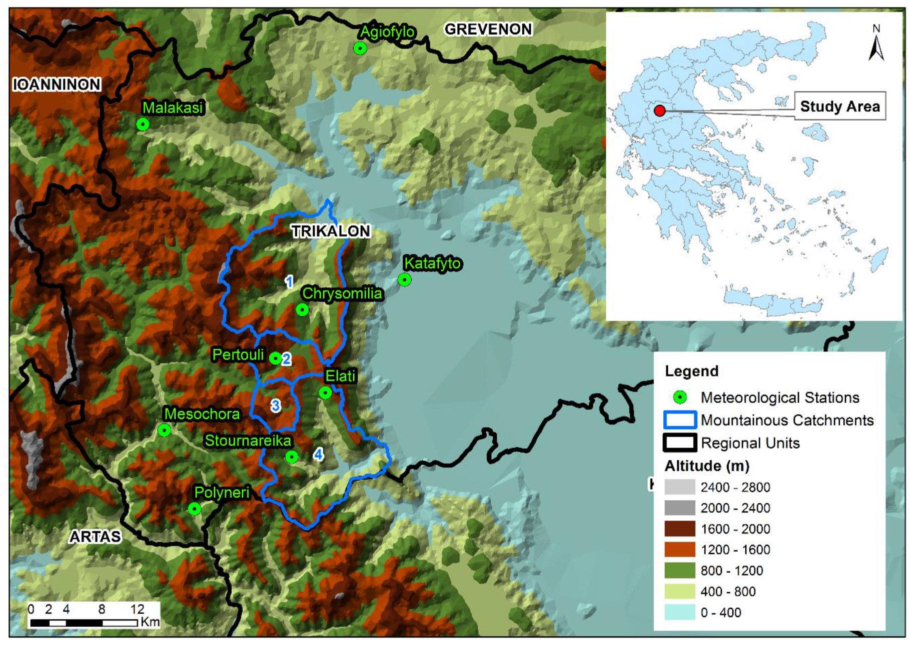
The study was conducted over the central Pindus mountain range, in Central Greece. The area is considered highly important from a hydrological point of view because it is located in the mountainous area of two hydrological basins (Pinios and Acheloos), which supply Central Greece with water, and where many hydropower dams have been constructed. For this purpose, a dense network of meteorological stations (compared to other regions in Greece) has been established, in mountainous terrain. The characteristics of the meteorological stations used in this study are given in Table 1.
Observations of monthly rainfall totals for a period of 55 years of rainfall (1961–2016) were used from all nine stations of the wider region (see Figure 1). These stations are equipped with pluviometer and Hellmann-type rain gauges (Fuess Meteorologische Instrumente KG, Königs Wusterhausen, Germany) with a precision of 0.1 mm. The data series are complete, that is, they have no missing values. Moreover, the instruments and observing practices were common among all stations used, and they remained the same during this study’s research. The double mass method and two parametric statistical tests (Student’s t-test and chi-squared test) were applied to adjust any heterogeneity of the rainfall data, and the details regarding these methods can be obtained from the WMO [31]. The latter tests demonstrated that the precipitation data were indeed homogeneous and ready to be entered into the subsequent procedures of the study.
These stations are operated by the Ministry of Environment & Energy (Agiofylo, Chrysomilia, Elati, Katafyto, and Malakasi), the Public Power Corporation (Mesochora, Polyneri, and Stournareika) and the University Forest Administration and Management Fund (Pertouli).
The study area is an area of increased importance, because it is located in the mountainous area of two hydrological basins (Pinios and Acheloos), which supply Central Greece with fresh water. The mountainous catchments examined within this study are (1) Klinovitikos, (2) Aspropotamos, (3) Korpos, and (4) Portaikos, as showed in Figure 1. Additionally, the basic morphometrical and hydrographical characteristics are given in Table 2.
The study area is characterized as mountainous, whereas the relief is rather intense. Regarding geology, the main rocks are flysch and limestones, quite vulnerable to landslides and weathering phenomena. The forest cover is high and distributed to the mountainous catchment as follows: (1) Klinovitikos, 66%; (2) Aspropotamos, 73%; (3) Korpos, 72%; and (4) Portaikos, 44%. The dominant forest species in the study area are Abies borisii-regis, Quercus frainetto, Quercus petraea, Pinus nigra, and Fagus Sylvatica. Moreover, the study region is of great environmental importance, belonging to the European nature conservation network Natura 2000 according to the criteria of Directive 92/43/EEC.
2.2. Trend Analysis
Time series of annual and seasonal rainfall were subjected to the Mann–Kendall test to detect possible trends over the period of 1961–2016. It is the most widely used test for trend analysis in climatological time series [32].
The Mann–Kendall test is a non-parametric statistical test to detect the presence of a monotonic increasing or decreasing trend within a time series [33,34]. The advantage of the non-parametric tests over the parametric tests is that they are robust and more suitable for non-normally distributed data with missing and extreme values, frequently encountered in environmental time series [35].
The Mann–Kendall test statistics S is calculated as:
where n is the number of data points, xi and xk are the data values in the time series j and k (j > k), respectively, and sign (xj − xi) is the sign function as follows:
The variance is computed as:
where n is the number of data points, P is the number of tied groups, the summary sign (P) indicates the summation over all tied groups, and ti is the number of data values in the Pth group. In case of no tied groups, this summary process can be ignored. A tied group is a set of sample data having the same value. In the case where the sample size n > 30, the standard normal test statistic Z is estimated by:
Positive values of Z indicate increasing trends, whereas negative Z values indicate decreasing trends. Trend testing is done at a specific significance level. When |Z| > Z1−a/2, the null hypothesis is rejected and a significant trend exists in the time series. The value of Z1−a/2 is obtained from the standard normal distribution table. In this study, the significance level a = 0.05 was used. At the 5% significance level, the null hypothesis of no trend is rejected if |Z| > 1.96.
Furthermore, a change-point analysis approach was applied, using the Change-Point Analyzer (CPA) [36]. This method iteratively uses a combination of cumulative sum charts (CUSUM) and bootstrapping to detect whether a change in the mean of the rainfall time series has taken place. A sudden change in the direction of the CUSUM indicates a sudden shift or change in the average. Additionally, trend magnitudes were computed by employing the Theil–Sen approach (TSA) [37,38], which is based on slope β, often referred to as Sen’s slope [38]. It is preferable to linear regression, because it limits the influence of outliers on the slope [39].
2.3. Spatial Mapping of Rainfall
Initially, the relationship between altitude and rainfall height (mm) for both an annual and a seasonal basis was evaluated using different types of trendlines (linear, logarithmic, polynomial, power, and exponential). Moreover, the spatial distribution was determined, applying multiple regression equation and taking into account not only the altitude but also the longitude and latitude. The multiple linear regression equation has the following form:
where P represents the rainfall (mm), a is constant, b1…b3 are coefficients obtained for each independent variable, X1 is longitude (°), X2 is latitude (°), and X3 is altitude (m).
Furthermore, the geostatistical interpolation method of ordinary kriging (spherical variogram) was employed, using the ArcGIS 10.2 software. At this point, it should be noted that geostatistical methods are more valid for increasing sample size. To this end, automatic points were generated in a 1 km × 1 km grid resolution within the catchments, using the Fishnet command of the ArcGIS 10.2 software’s Data Management toolbar. Therefore, rainfall height was calculated for each point and all seasons, based on the multiple regression equation described above and the calculation of the individual variables for each point.
Finally, cross-validation was performed, in order to compare results of rainfall spatial interpolation derived from ordinary kriging with other spatial interpolation methods, for example, inverse distance weighting (IDW), radial basis function (RBF), and universal kriging (UK), and a combination of variograms (spherical, exponential), using the Geostatistical Wizard tool of ArcGIS [40].
Cross-validation is any of various similar model validation techniques for assessing how the results of a statistical analysis will generalize to an independent dataset. It is mainly used in settings where the goal is prediction, and where one wants to estimate how accurately a predictive model will perform in practice. In a prediction problem, a model is usually given a dataset of known data on which training is run (training dataset), and a dataset of unknown data (or first seen data) against which the model is tested. The goal of cross-validation is to test the model’s ability to predict new data that were not used in estimating it, in order to flag problems like overfitting and to give an insight on how the model will generalize to an independent dataset.
The root mean square error (RMSE) and mean error were used as evaluation indexes in this case study. The mathematical description of these indexes is given below:
where n is the number of observations, and xi and yi are the observed and interpolated rainfall values, respectively, for i = 1, 2 … n. The RMSE is considered one of the most reliable indexes because it depicts the deviation from the truth rather than the mean value, as in the case of standard deviation. The RMSE gives the weighted variations (residuals) in errors between the estimated and observed values, whereas mean error measures the weighted average magnitude of the errors. Mean error is the most natural and unambiguous measure of average error magnitude [41,42]. RMSE, on the other hand, is one of the most widely used error measures [43].
3. Results
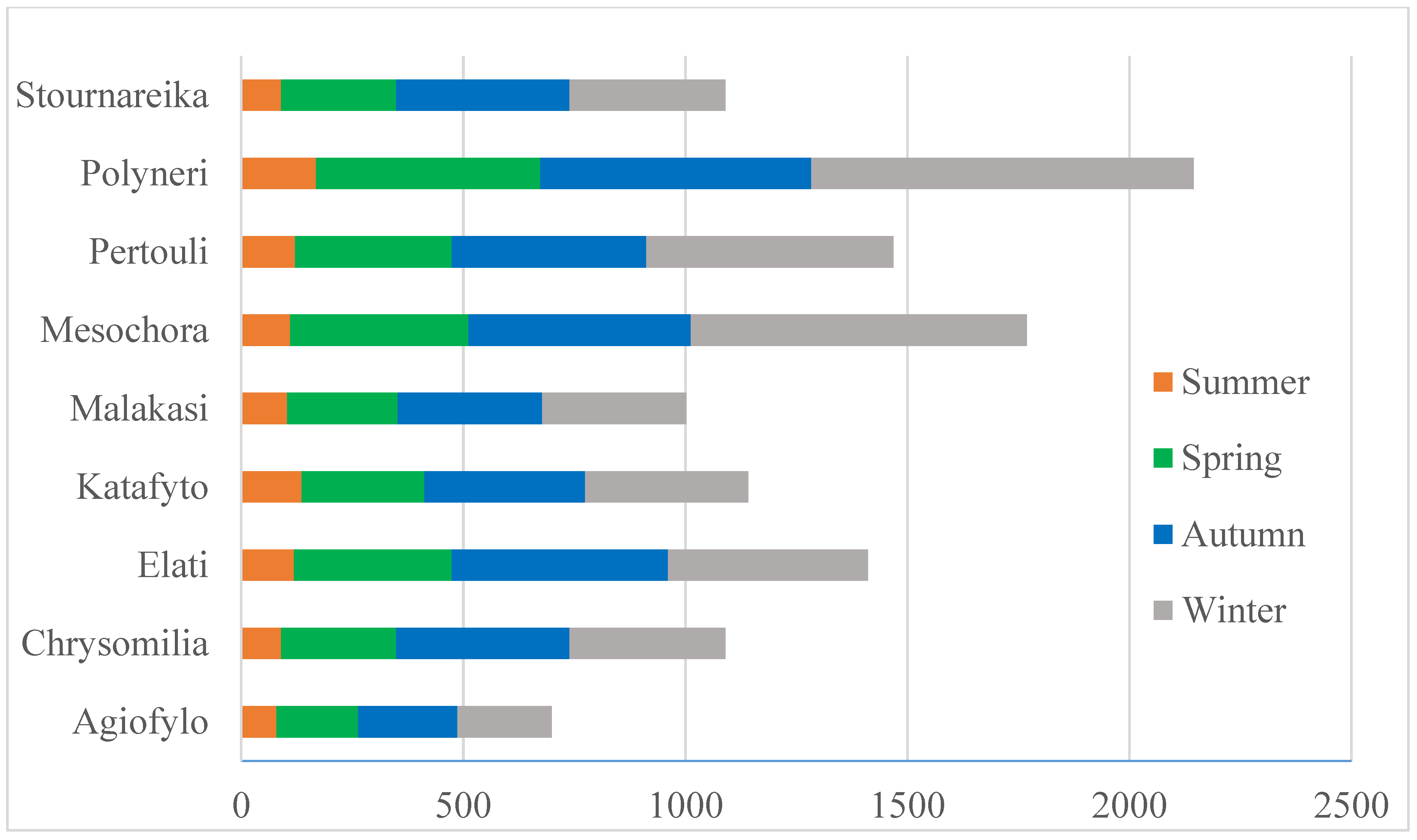
The rainfall pattern in the case study area demonstrated certain particularities and varied greatly in both space and time, in line with the main characteristics of the climate type in the Mediterranean basin. The seasonal distribution of rainfall based on the examined meteorological stations’ data is shown in Figure 2. As depicted, 35% of the annual rainfall occurs during winter, 32% in autumn, 24% in spring, and only 9% in summer.
The results of the Mann–Kendall statistics test indicated that most of the meteorological stations (around 67%) recorded a downward trend in annual rainfall, which could be considered as statistically significant for the Katafyto station. In addition, decreasing trends of rainfall time series were recorded in winter and autumn for most of the stations. During spring, half of the stations revealed a decreasing trend, whereas the other half revealed an increasing one. Finally, summer was the only time season when rainfall trends were recorded increasing in most of the stations.
Detailed results of the application of the Mann–Kendall test are given in Table 3. The upward arrow ↑ indicates an increasing trend, whereas the downward arrow ↓ indicates a decreasing one. Furthermore, the light grey cell color shows that the trend is not statistically significant (for a significance level of a = 0.05), whereas the dark grey color shows a statistically significant trend. In addition, the number within the parenthesis indicates the time of occurrence for changes in the mean of the rainfall time series.
As shown in Table 3, the rainfall non-stationarity starts to occur in the middle of 1960s for the annual, autumn, spring, and summer rainfalls and the early 1970s for the winter rainfall in most of the stations.
Moreover, Sen’s slope was used to compute the trend magnitude per decade, which ranged from approximately −5.3% to +1.5% (average −1.9%) in annual rainfalls, from −14.5% to +7.5% (average −3.2%) in winter, from −4.7% to +5.5% (average +0.7%) in autumn, from −4.2% to +3.6% (average +0.2%) in spring, and from −0.3% to +4.8% (average +2.4%) in summer. Detailed results for each station are given in the next table (see Table 4).
The investigation of the relationships between the variation of rainfall and altitude showed that the derived coefficients of determination are rather low. This indicates that only a small percentage (19–25%) of rainfall variation in the study area was due to the change in altitude. Furthermore, it was observed that the power trendline performed the best fit in all cases. In the equations below (see Table 5), y is the rainfall (mm) and x is altitude (m).
For that reason, the spatial variability of both seasonal and annual rainfall was assessed using a multiple regression analysis. All the necessary factors affecting rainfalls were included into the multiple regression procedure, including longitude, latitude, and altitude. The coefficient obtained for each factor, based on a regression analysis, is given in Table 6.
It is noteworthy that the multiple regression model can explain 62.2% of the spatial variability of the annual rainfall, 58.9% of variability in winter, 75.9% of variability in autumn, 55.1% of variability in spring, and 32.2% of variability in summer. In order to evaluate the statistical significance of the examined factors, p-values were estimated (see Table 7). In cases where the significant level of the examined factor is less than 95% (p > 0.05), the factor should be eliminated from the model and the multi-linear regression must be performed again. In this study, the p-values for all factors were less than 0.05, which means a strong presumption against null hypothesis.
Furthermore, regarding the results of cross validation amongst different spatial interpolation methods it was revealed that better results were achieved by Ordinary Kriging combined with spherical semivariogram (Table 8).
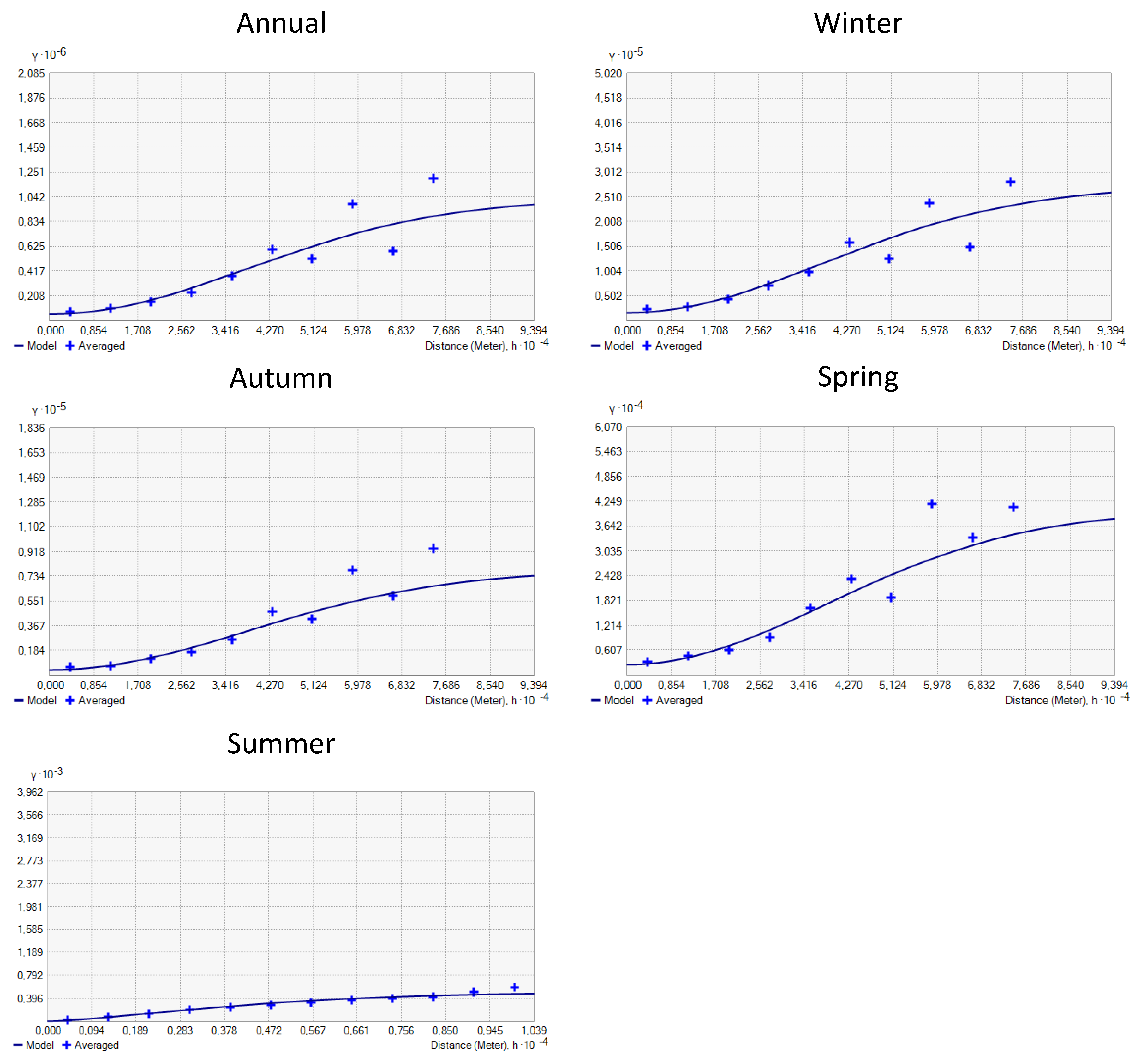
The semivariogram/covariance cloud tool shows the empirical semivariogram and covariance values for all pairs of locations within a dataset and plots them as a function of the distance that separates the two locations. It can be used to examine the local characteristics of spatial autocorrelation within a dataset and look for local outliers. The selection of lag size has an important effect on the semivariogram. If the lag size is too large, the short-range autocorrelation may be masked, whereas if the lag size is too small, there may be many empty bins. A rule of thumb is to multiply the lag size times the number of lags, which should be about half of the largest distance among all points.
Important characteristics of the semivariogram are also the nugget and the partial sill. The nugget is a parameter of covariance or semivariogram model that represents independent error, and a microscale variation at spatial scales that are too fine to detect. As for the partial sill, it is a parameter that represents the variance of a spatially autocorrelated process without any nugget effect. These parameters for the spherical variogram that was used in this study are given in the following table (see Table 9).
Regarding the semivariograms (see Figure 3), it can be assumed that the phenomenon to estimate is smooth (i.e., rainfall values change gradually with the distance). The semivariogram represents the continuity structure quite well also. Additionally, the semivariogram diagrams showed that the samples did not show autocorrelation in any direction.
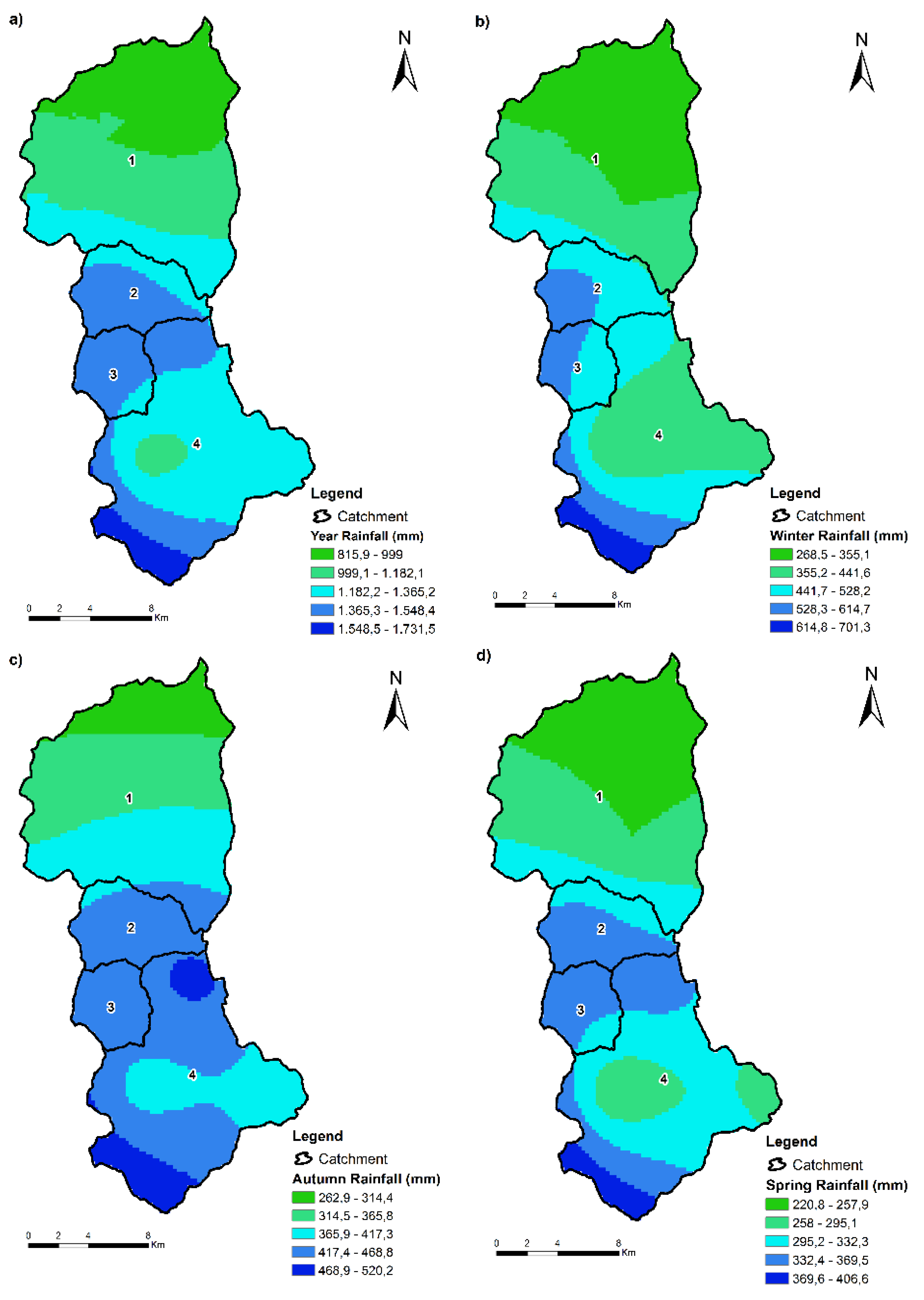
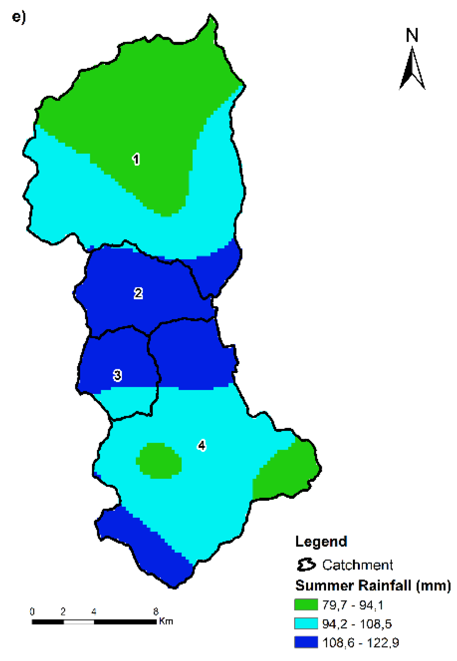
The rainfall spatial distribution maps over the mountainous catchment of the study area were produced using ordinary kriging and are given in the following figure (see Figure 4).
4. Conclusions
Rainfall variability is crucial for rational water resource management especially in Mediterranean countries, such as Greece, with rainfalls presenting temporal and spatial variation. In this study, monthly rainfall data from nine meteorological stations in the central Pindus mountain range were collected and analyzed for the period of 1961–2016. The conclusions reached are summarized below:
- ◾
- Rainfall is characterized by great seasonal variability. Of the whole year’s rainfall, 35% falls during winter, 32% during autumn, 24% during spring, and 9% during summer. Previous studies [44,45,46] have shown that there is a high degree of correlation between seasonal rainfall amounts and seasonal rainy days and the corresponding frequency of cyclonic circulation types at 500 hPa.
- ◾
- Regarding the results of the Mann–Kendall test, it is highlighted that at most of the examined meteorological stations, decreasing trends were recorded on an annual basis; winter and spring rainfalls showed a decreasing trend, as well. As for the autumn and summer rainfalls, increasing trends were recorded in most stations. The above-mentioned trends are not statistically significant, except for the annual rainfall decreasing trend at the Katafyto station and the winter rainfall decreasing trends at the Katafyto and Pertouli stations. In addition, it was found that rainfall non-stationarity starts to occur in the middle of the 1960s for the annual, autumn, spring, and summer rainfalls and the early 1970s for the winter rainfall in most of the stations. Finally, the average trend magnitude per decade, using Sen’s slope method, was −1.9% for the annual rainfall, −3.2% for the winter rainfall, +0.7% for the autumn rainfall, +0.2% for the spring rainfall, and +2.4 for the summer rainfall. The observed downward trends in rainfall in Greece was linked mainly to a rising trend in the hemispheric circulation modes of the North Atlantic Oscillation Index and its connection with the Mediterranean Oscillation Index [47]. In addition, the link between precipitation variability in Greece and the Mediterranean pressure oscillation is very reasonable from a physical point of view.
- ◾
- The ordinary kriging method gives better results in spatial rainfall mapping in the study area in comparison with other spatial interpolation methods. The spatial variability in rainfall is extremely high. The relationship between geomorphological factors (longitude, latitude, and altitude) and rainfall was obtained and proposed using a multiple regression technique. The results indicated that the developed regression models could better explain the variability of rainfall in autumn and winter, rather than in spring and summer. Moreover, the spatial distribution maps obtained using ordinary kriging through the GIS software revealed a wide range of rainfalls (for all seasons) through the catchments, whereas many different zones of rainfalls could be recognized. These maps are easy to produce for every area of interest and are reliable and useful for various stakeholders.
- ◾
- According the rainfall pattern of the study area, there is a lack of water during summer months and great differences of rainfall amounts between the mountainous areas and the lowlands. The need for the rational management of mountainous catchments is now a necessity. Appropriate silvicultural treatments must be applied in order to achieve an all-aged forest stand structure, which can increase water production from the mountainous catchments [48,49]. Additionally, stream regulation using check dams could have a positive effect on water availability. After siltation waters have infiltrated through the deposits, they act as ideal artificial aquifers. To accomplish this goal, appropriate pipelines to the lower body of the check dams must be constructed. The retained water is supplied with piping and by natural flow to the areas that have a demand. This method of water conservation provides clean and filtered water and avoids evaporation losses [50].
Author Contributions
S.S. analyzed the GIS data, investigated the spatial distribution of rainfall, and wrote the paper, whereas D.S. collected the meteorological data and applied the Mann–Kendall statistical test.
Funding
This research received no external funding.
Conflicts of Interest
The authors declare no conflict of interest.
References
- Maheras, P.; Anagnostopoulou, C. Circulation types and their influence on the interannual variability and precipitation changes in Greece. In Mediterranean Climate; Springer: Berlin/Heidelberg, Germany, 2003; pp. 215–239. [Google Scholar]
- Tolika, K.; Maheras, P.; Anagnostopoulou, C. The exceptionally wet year of 2014 over Greece: A statistical and synoptical-atmospheric analysis over the region of Thessaloniki. Theor. Appl. Climatol. 2017, 132, 809–821. [Google Scholar] [CrossRef]
- Xoplaki, E.; Luterbacher, J.; Burkard, R.; Patrikas, I.; Maheras, P. Connection between the large-scale 500 hPa geopotential height fields and precipitation over Greece during wintertime. Clim. Res. 2000, 14, 129–146. [Google Scholar] [CrossRef]
- Metaxas, D.A. Evidence on the importance of diabatic heating as a divergence factor in the Mediterranean. Arch. Meteorol. Geophys. Bioklimatol. 1978, 27, 69–80. [Google Scholar] [CrossRef]
- Stathis, D. The role of topography in the distribution of precipitation over mountainous Greece as reveal by principal component analysis. J. Meteorol. 1999, 24, 50–56. [Google Scholar]
- Buytaert, W.; Celleri, R.; Willems, P.; De Bievre, B.; Wyseure, G. Spatial and temporal rainfall variability in mountainous areas: A case study from the south Ecuadorian Andes. J. Hydrol. 2006, 329, 413–421. [Google Scholar] [CrossRef] [Green Version]
- Stathis, D.; Myronidis, D. Principal component analysis of precipitation in Thessaly region (Central Greece). Glob. NEST J. 2009, 11, 467–476. [Google Scholar]
- Maris, F.; Kitikidou, K.; Angelidis, P.; Potouridis, S. Kriging interpolation method for estimation of continuous spatial distribution of precipitation in Cyprus. Br. J. Appl. Sci. Technol. 2013, 3, 1286–1300. [Google Scholar] [CrossRef]
- De Amorim Borges, P.; Franke, J.; da Anunciação, Y.M.T.; Weiss, H.; Bernhofer, C. Comparison of spatial interpolation methods for the estimation of precipitation distribution in Distrito Federal, Brazil. Theor. Appl. Climatol. 2016, 123, 335–348. [Google Scholar] [CrossRef]
- Paparrizos, S.; Maris, F.; Matzarakis, A. A downscaling technique for climatological data in areas with complex topography and limited data. Int. J. Eng. Res. Dev. 2016, 12, 17–23. [Google Scholar]
- Syed, M.A.; Al Amin, M. Geospatial modeling for investigating spatial pattern and change trend of temperature and rainfall. Climate 2016, 4, 21. [Google Scholar] [CrossRef]
- Arnell, N.W.; Goslin, S.N. The impacts of climate change on river flood risk at the global scale. Clim. Chang. 2016, 134, 387–401. [Google Scholar] [CrossRef]
- Simonneaux, V.; Cheggour, A.; Deschamps, C.; Mouillot, F.; Cerdan, O.; Le Bissonnais, Y. Land use and climate change effects on soil erosion in a semi-arid mountainous watershed (High Atlas, Morocco). J. Arid Environ. 2015, 122, 64–75. [Google Scholar] [CrossRef] [Green Version]
- Anagnostopoulou, C. Drought episodes over Greece as simulated by dynamical and statistical downscaling approaches. Theor. Appl. Climatol. 2017, 129, 587–605. [Google Scholar] [CrossRef]
- Blanc, E.; Reilly, J. Approaches to assessing climate change impacts on agriculture: An overview of the debate. Rev. Environ. Econ. Policy 2017, 11, 247–257. [Google Scholar] [CrossRef]
- Michailidou, A.V.; Vlachokostas, C.; Moussiopoulos, Ν. Interactions between climate change and the tourism sector: Multiple-criteria decision analysis to assess mitigation and adaptation options in tourism areas. Tour. Manag. 2016, 55, 1–12. [Google Scholar] [CrossRef]
- Theodossiou, N. Assessing the Impacts of Climate Change on the Sustainability of Groundwater Aquifers. Application in Moudania Aquifer in N. Greece. Environ. Process. 2016, 3, 1045–1061. [Google Scholar] [CrossRef]
- Kalabokidis, K.; Palaiologou, P.; Gerasopoulos, E.; Giannakopoulos, C.; Kostopoulou, E.; Zerefos, C. Effect of climate change projections on forest fire behavior and values-at-risk in Southwestern Greece. Forests 2015, 6, 2214–2240. [Google Scholar] [CrossRef]
- Intergovernmental Panel on Climate Change (IPCC). Climate Change 2013: The Physical Science Basis. Contribution of Working Group I to the Fifth Assessment Report of the Intergovernmental Panel on Climate Change; Cambridge University Press: Cambridge, UK, 2013. [Google Scholar]
- Cox, P.M.; Betts, R.A.; Jones, C.D.; Spall, S.A.; Totterdell, I.J. Acceleration of global warming due to carbon-cycle feedbacks in a coupled climate model. Nature 2000, 408, 184–187. [Google Scholar] [CrossRef] [PubMed]
- Solomon, S.; Plattner, G.K.; Knutti, R.; Friedlingstein, P. Irreversible climate change due to carbon dioxide emissions. Proc. Natl. Acad. Sci. USA 2009, 106, 1704–1709. [Google Scholar] [CrossRef] [PubMed] [Green Version]
- Giorgi, F.; Lionello, P. Climate change projections for the Mediterranean region. Glob. Planet. Chang. 2008, 63, 90–104. [Google Scholar] [CrossRef]
- Sahsamanoglou, H.; Makrogiannis, T.; Hatzianastasiou, N.; Rammos, N. Long term change of precipitation over the Balkan Peninsula. In Eastern Europe and Global Change; European Commission: Brussels, Belgium, 1997; pp. 111–124. [Google Scholar]
- Maheras, P.; Tolika, K.; Anagnostopoulou, C.; Vafiadis, M.; Patrikas, I.; Flocas, H. On the relationships between circulation types and changes in rainfall variability in Greece. Int. J. Climatol. 2004, 24, 1695–1712. [Google Scholar] [CrossRef] [Green Version]
- Nastos, P.T.; Zerefos, C.S. Spatial and temporal variability of consecutive dry and wet days in Greece. Atmos. Res. 2009, 94, 616–628. [Google Scholar] [CrossRef]
- Mavromatis, T.; Stathis, D. Response of the water balance in Greece to temperature and precipitation trends. Theor. Appl. Climatol. 2011, 104, 13–24. [Google Scholar] [CrossRef]
- Stefanidis, S.; Chatzichristaki, C. Response of soil erosion in a mountainous catchment to temperature and precipitation trends. Carpathian J. Earth Environ. Sci. 2017, 12, 35–39. [Google Scholar]
- Markonis, Y.; Batelis, S.C.; Dimakos, Y.; Moschou, E.; Koutsoyiannis, D. Temporal and spatial variability of rainfall over Greece. Theor. Appl. Climatol. 2017, 130, 217–232. [Google Scholar] [CrossRef]
- Tolika, K.; Zanis, P.; Anagnostopoulou, C. Regional climate change scenarios for Greece: Future temperature and precipitation projections from ensembles of RCMs. Glob. NEST J. 2012, 14, 407–421. [Google Scholar]
- Paparrizos, S.; Maris, F.; Matzarakis, A. Integrated analysis of present and future responses of precipitation over selected Greek areas with different climate conditions. Atmos. Res. 2016, 169, 199–208. [Google Scholar] [CrossRef]
- World Meteorological Organization (WMO). Guidelines on the Quality Control of Surface Climatological Data; WCP-85; WMO: Geneva, Switzerland, 1986. [Google Scholar]
- Goossens, C.; Berger, A. Annual and seasonal climatic variations over the northern hemisphere and Europe during the last century. Ann. Geophys. 1986, 4, 385–400. [Google Scholar]
- Mann, B. Nonparametric tests against trend. Econom. J. Econom. Soc. 1945, 13, 245–259. [Google Scholar] [CrossRef]
- Kendall, M. Multivariate Analysis; Charles Griffin: London, UK, 1975. [Google Scholar]
- Sicard, P.; Dalstein-Richier, L. Health and vitality assessment of two common pine species in the context of climate change in southern Europe. Environ. Res. 2015, 137, 235–245. [Google Scholar] [CrossRef] [PubMed]
- Taylor, W. Change-Point Analyzer 2.0 Shareware Program; Taylor Enterprises: Libertyville, IL, USA, 2000; Available online: http://www.variation.com/cpa/ (accessed on 19 July 2018).
- Thiel, H. A rank-invariant method of linear and polynomial regression analysis, part 3. In Advanced Studies in Theoretical and Applied Econometrics; Springer: Berlin, Germany, 1992; pp. 345–381. [Google Scholar]
- Sen, P.K. Estimates of the regression coefficients based on Kendall’s tau. J. Am. Stat. Assoc. 1968, 63, 1379–1389. [Google Scholar] [CrossRef]
- Hirsch, R.M.; Slack, J.R.; Smith, R.A. Techniques of trend analysis for monthly water quality data. Water Resour. Res. 1982, 18, 107–121. [Google Scholar] [CrossRef]
- Goovaerts, P. Geostatistical approaches for incorporating elevation into the spatial interpolation of rainfall. J. Hydrol. 2000, 228, 113–129. [Google Scholar] [CrossRef] [Green Version]
- Willmott, J.; Matsuura, K. Advantages of the mean absolute error (MAE) over the root mean square error (RMSE) in assessing average model performance. Clim. Res. 2015, 30, 79–82. [Google Scholar] [CrossRef]
- Chai, T.; Draxler, R. Root mean square error (RMSE) or mean absolute error (MAE)?—Arguments against avoiding RMSE in the literature. Geosci. Model Dev. 2014, 7, 1247–1250. [Google Scholar] [CrossRef]
- Mavromatis, T. Spatial resolution effects on crop yield forecasts: An application to rainfed wheat yield in north Greece with CERES-Wheat. Agric. Syst. 2016, 143, 38–48. [Google Scholar] [CrossRef]
- Norrant-Romand, C.; Douguédroit, A. Significant rainfall decreases and variations of the atmospheric circulation in the Mediterranean (1950–2000). Reg. Environ. Chang. 2014, 14, 1725–1741. [Google Scholar] [CrossRef]
- Casado, M.J.; Pastor, M.A. Circulation types and winter precipitation in Spain. Int. J. Climatol. 2016, 36, 2727–2742. [Google Scholar] [CrossRef]
- Putniković, S.; Tošić, I. Relationship between atmospheric circulation weather types and seasonal precipitation in Serbia. Meteorol. Atmos. Phys. 2017. [CrossRef]
- Feidas, H.; Noulopoulos, C.; Makrogiannis, T.; Bora-Senta, E. Trend analysis of precipitation time series in Greece and their relationship with circulation using surface and satellite data. Theor. Appl. Climatol. 2007, 87, 155–177. [Google Scholar] [CrossRef]
- Kotoulas, D. Hydrological influences of forests in torrent catchment regions of Greece. Schweiz. Z. Forstwes. 1980, 131, 617–626. [Google Scholar]
- Gatzojannis, S.; Stefanidis, P.; Kalabokidis, K. An inventory and evaluation methodology for non-Tiber functions of forests. Mitt. Abt. Forstl. Biom. 2001, 1, 3–49. [Google Scholar]
- Kotoulas, D. The possibilities of increase water supply in Greece. Sci. Ann. Dep. For. Nat. Environ. 1992, LE, 141–149. (In Greek) [Google Scholar]
Figure 1.
The study area and location of stations.

Figure 2.
Seasonal distribution of rainfall.

Figure 3.
Spherical semivariograms of ordinary kriging interpolation models for annual and seasonal rainfalls.
Figure 3.
Spherical semivariograms of ordinary kriging interpolation models for annual and seasonal rainfalls.

Figure 4.
Spatial distribution of (a) annual, (b) winter, (c) autumn, (d) spring and (e) summer rainfall over the study area.
Figure 4.
Spatial distribution of (a) annual, (b) winter, (c) autumn, (d) spring and (e) summer rainfall over the study area.


Table 1.
Meteorological stations in the study area.
| A/A | Meteorological Station | Coordinates | Altitude (m) | Period (years) | |
|---|---|---|---|---|---|
| Longitude(o) | Latitude(o) | ||||
| 1 | Agiofylo | 21.34 | 39.52 | 581 | 1961–2016 |
| 2 | Chrysomilia | 21.3 | 39.36 | 940 | 1961–2016 |
| 3 | Elati | 21.32 | 39.51 | 900 | 1961–2016 |
| 4 | Katafyto | 21.28 | 39.38 | 980 | 1961–2016 |
| 5 | Malakasi | 21.17 | 39.47 | 849 | 1961–2016 |
| 6 | Mesochora | 21.20 | 39.26 | 849 | 1961–2016 |
| 7 | Pertouli | 21.28 | 39.33 | 1180 | 1961–2016 |
| 8 | Polyneri | 21.22 | 39.34 | 801 | 1961–2016 |
| 9 | Stournareika | 21.29 | 39.28 | 761 | 1961–2016 |
Table 2.
Morphometrical and hydrographical characteristics of the mountainous catchments.
| Catchment Name | Klinovitikos | Aspropotamos | Korpos | Portaikos | |||
|---|---|---|---|---|---|---|---|
| Code | (1) | (2) | (3) | (4) | |||
| A/A | Morphometrical Characteristics | Symbol | Units | ||||
| 1 | Area | F | km2 | 171.1 | 36.3 | 23.7 | 136.4 |
| 2 | Perimeter | U | km | 61.7 | 28.1 | 20.1 | 60 |
| 3 | Minimum elevation | Hmin | m | 320 | 1020 | 1020 | 240 |
| 4 | Maximum elevation | Hmax | m | 2204 | 2074 | 1721 | 1862 |
| 5 | Mean elevation | Hmed | m | 1112 | 1420 | 1397 | 963 |
| 6 | Mean catchment slope | Jλ | % | 48.4 | 41.6 | 39.3 | 52.93 |
| Hydrographic Characteristics | |||||||
| 7 | Density of hydrographic network | D | km/km2 | 2.86 | 3.13 | 3.36 | 2.69 |
| 8 | Main stream length | L | km | 20.2 | 12.4 | 8.3 | 16.9 |
| 9 | Main stream slope | Jκ | % | 6.5 | 5.6 | 9.6 | 7.8 |
Table 3.
Trend detection using the Mann–Kendall test and the change-point analysis.
| a/a | Meteorological Station | Period | ||||
|---|---|---|---|---|---|---|
| Annual | Winter | Autumn | Spring | Summer | ||
| 1 | Agiofylo | ↑ (86) | ↑ (66) | ↑ (96) | ↑ (62) | ↑ (62) |
| 2 | Chrysomilia | ↓ (67) | ↓ (89) | ↑ (62) | ↑ (64) | ↑ (68) |
| 3 | Elati | ↓ (65) | ↓ (88) | ↓ (63) | ↓ (96) | ↑ (62) |
| 4 | Katafyto | ↓ (75) | ↓ (01) | ↓ (63) | ↓ (64) | ↑ (63) |
| 5 | Malakasi | ↓ (65) | ↓ (74) | ↓ (63) | ↓ (64) | ↑ (62) |
| 6 | Mesochora | ↑ (67) | ↓ (72) | ↑ (73) | ↑ (71) | ↑ (68) |
| 7 | Pertouli | ↓ (65) | ↓ (71) | ↑ (62) | ↓ (62) | ↓ (71) |
| 8 | Polyneri | ↑ (64) | ↓ (70) | ↑ (62) | ↑ (64) | ↑ (63) |
| 9 | Stournareika | ↓ (64) | ↓ (70) | ↑ (63) | ↑ (63) | ↓ (70) |
Table 4.
Trend magnitude (%) per decade using Sen’s slope method.
| a/a | Meteorological Station | Trend Magnitude (% per Decade) | ||||
|---|---|---|---|---|---|---|
| Annual | Winter | Autumn | Spring | Summer | ||
| 1 | Agiofylo | −5.3% | 7.5% | 5.3% | 2.9% | 4.6% |
| 2 | Chrysomilia | −0.4% | −2.1% | 0.9% | 2.3% | 1.3% |
| 3 | Elati | −4.3% | −2.2% | −0.2% | −4.2% | 0.1% |
| 4 | Katafyto | −5.1% | −14.5% | −4.7% | −0.3% | 9.7% |
| 5 | Malakasi | −0.7% | −3.7% | −1.2% | −1.5% | 4.8% |
| 6 | Mesochora | 1.5% | −1.9% | 5.5% | 3.6% | 0.9% |
| 7 | Pertouli | −3.1% | −5.5% | 0.3% | −3.8% | −0.3% |
| 8 | Polyneri | 1.4% | −3.1% | 0.1% | 1.5% | 0.8% |
| 9 | Stournareika | −1.1% | −2.9% | 0.4% | 0.9% | −0.3% |
Table 5.
Relationship between rainfall and altitude.
| Trend Equation | R2 | |
|---|---|---|
| Annual | y = 6.14x0.8 | 0.21 |
| Winter | y = 0.60x0.9 | 0.18 |
| Autumn | y = 2.63x0.6 | 0.25 |
| Spring | y = 2.94x0.7 | 0.19 |
| Summer | y = 2.57x0.6 | 0.21 |
Table 6.
Coefficients of multiple regression models and statistics.
| Coefficients | |||||
|---|---|---|---|---|---|
| Annual | Winter | Autumn | Spring | Summer | |
| a | 77,660 | 35,750 | 22,056 | 16,815 | 2963 |
| b1 | −0.018 | −0.010 | −0.003 | −0.004 | −0.001 |
| b2 | −0.016 | −0.007 | −0.005 | −0.003 | −0.001 |
| b3 | 0.21 | 0.06 | 0.07 | 0.05 | 0.03 |
| Adjusted R2 | 0.62 | 0.59 | 0.76 | 0.55 | 0.32 |
Table 7.
Output p-values of the examined coefficients.
| p-Values | |||||
|---|---|---|---|---|---|
| Annual | Winter | Autumn | Spring | Summer | |
| a | 0.021 | 0.031 | 0.005 | 0.030 | 0.028 |
| b1 | 0.046 | 0.038 | 0.026 | 0.028 | 0.046 |
| b2 | 0.028 | 0.041 | 0.007 | 0.041 | 0.031 |
| b3 | 0.048 | 0.049 | 0.039 | 0.044 | 0.049 |
Table 8.
Cross-validation results from the interpolation of annual and seasonal rainfall.
| Inverse Distance Weighting | |||||
|---|---|---|---|---|---|
| Annual | Winter | Autumn | Spring | Summer | |
| Mean Error | 78.52 | 33.82 | 24.57 | 16.98 | 3.04 |
| RMSE | 315.04 | 148.19 | 95.99 | 63.67 | 24.79 |
| Radial Basis Function | |||||
| Mean Error | 38.78 | 16.87 | 12.28 | 8.08 | 1.42 |
| RMSE | 282.96 | 128.60 | 83.62 | 53.87 | 20.38 |
| Ordinary Kriging (Spherical) | |||||
| Mean Error | 16.58 | 7.32 | 4.58 | 3.35 | 0.38 |
| RMSE | 254.24 | 117.13 | 76.57 | 48.92 | 20.22 |
| Ordinary Kriging (Exponential) | |||||
| Mean Error | 22.02 | 9.55 | 6.93 | 4.68 | 0.43 |
| RMSE | 268.34 | 123.06 | 79.76 | 51.44 | 22.86 |
| Universal Kriging (Spherical) | |||||
| Mean Error | 16.62 | 8.11 | −4.76 | −8.85 | −2.41 |
| RMSE | 255.70 | 119.20 | 77.80 | 73.26 | 25.88 |
| Universal Kriging (Exponential) | |||||
| Mean Error | −49.77 | −27.67 | −12.50 | 4.52 | −5.42 |
| RMSE | 384.76 | 192.78 | 110.46 | 52.60 | 29.54 |
Table 9.
Variogram Statistics.
| Parameter | Annual | Winter | Autumn | Spring | Summer |
|---|---|---|---|---|---|
| Nugget | 0 | 0 | 0 | 0 | 283.01 |
| Partial Sill | 678185.10 | 7828.59 | 93943.10 | 27528.71 | 493.07 |
| Lag size | 7828.59 | 7828.59 | 7828.59 | 7828.59 | 2100.93 |
Table 10.
Annual and seasonal rainfall (mm) ranges in the catchments of the study area.
| Annual | Winter | Autumn | Spring | Summer | |||||||
|---|---|---|---|---|---|---|---|---|---|---|---|
| a/a | Catchment | Min | Max | Min | Max | Min | Max | Min | Max | Min | Max |
| 1 | Klinovitikos | 815.9 | 1336.7 | 268.5 | 494.6 | 262.9 | 449.1 | 220.8 | 328.6 | 79.7 | 115.1 |
| 2 | Aspropotamos | 1279.1 | 1483.2 | 434.7 | 562.7 | 406.5 | 463.9 | 308.4 | 351.9 | 106.5 | 121.6 |
| 3 | Korpos | 1281.2 | 1530.4 | 437.2 | 592.0 | 428.9 | 456.4 | 308.2 | 358.9 | 101.9 | 117.7 |
| 4 | Portaikos | 1100.2 | 1731.5 | 355.7 | 703.0 | 381.6 | 520.2 | 261.1 | 406.6 | 88.1 | 122.9 |
© 2018 by the authors. Licensee MDPI, Basel, Switzerland. This article is an open access article distributed under the terms and conditions of the Creative Commons Attribution (CC BY) license (http://creativecommons.org/licenses/by/4.0/).
Share and Cite
MDPI and ACS Style
Stefanidis, S.; Stathis, D. Spatial and Temporal Rainfall Variability over the Mountainous Central Pindus (Greece). Climate 2018, 6, 75. https://0-doi-org.brum.beds.ac.uk/10.3390/cli6030075
AMA Style
Stefanidis S, Stathis D. Spatial and Temporal Rainfall Variability over the Mountainous Central Pindus (Greece). Climate. 2018; 6(3):75. https://0-doi-org.brum.beds.ac.uk/10.3390/cli6030075
Chicago/Turabian StyleStefanidis, Stefanos, and Dimitrios Stathis. 2018. "Spatial and Temporal Rainfall Variability over the Mountainous Central Pindus (Greece)" Climate 6, no. 3: 75. https://0-doi-org.brum.beds.ac.uk/10.3390/cli6030075
Note that from the first issue of 2016, this journal uses article numbers instead of page numbers. See further details here.