Time Series Analysis of MODIS-Derived NDVI for the Hluhluwe-Imfolozi Park, South Africa: Impact of Recent Intense Drought


Department of Geography and Environmental Studies, University of Zululand, KwaDlangezwa 3886, South Africa
*
Author to whom correspondence should be addressed.
Climate 2018, 6(4), 95; https://0-doi-org.brum.beds.ac.uk/10.3390/cli6040095
Submission received: 8 October 2018
/
Revised: 7 November 2018
/
Accepted: 14 November 2018
/
Published: 30 November 2018
(This article belongs to the Special Issue Climate Variability and Change in the 21th Century)
Abstract
:The variability of temperature and precipitation influenced by El Niño-Southern Oscillation (ENSO) is potentially one of key factors contributing to vegetation product in southern Africa. Thus, understanding large-scale ocean–atmospheric phenomena like the ENSO and Indian Ocean Dipole/Dipole Mode Index (DMI) is important. In this study, 16 years (2002–2017) of Moderate Resolution Imaging Spectroradiometer (MODIS) Terra/Aqua 16-day normalized difference vegetation index (NDVI), extracted and processed using JavaScript code editor in the Google Earth Engine (GEE) platform was used to analyze the vegetation response pattern of the oldest proclaimed nature reserve in Africa, the Hluhluwe-iMfolozi Park (HiP) to climatic variability. The MODIS enhanced vegetation index (EVI), burned area index (BAI), and normalized difference infrared index (NDII) were also analyzed. The study used the Modern Retrospective Analysis for the Research Application (MERRA) model monthly mean soil temperature and precipitations. The Global Land Data Assimilation System (GLDAS) evapotranspiration (ET) data were used to investigate the HiP vegetation water stress. The region in the southern part of the HiP which has land cover dominated by savanna experienced the most impact of the strong El Niño. Both the HiP NDVI inter-annual Mann–Kendal trend test and sequential Mann–Kendall (SQ-MK) test indicated a significant downward trend during the El Niño years of 2003 and 2014–2015. The SQ-MK significant trend turning point which was thought to be associated with the 2014–2015 El Niño periods begun in November 2012. The wavelet coherence and coherence phase indicated a positive teleconnection/correlation between soil temperatures, precipitation, soil moisture (NDII), and ET. This was explained by a dominant in-phase relationship between the NDVI and climatic parameters especially at a period band of 8–16 months.
Keywords:
drought; NDVI; ENSO; wavelet; time series analysis; Hluhluwe-iMfolozi Park; Google Earth Engine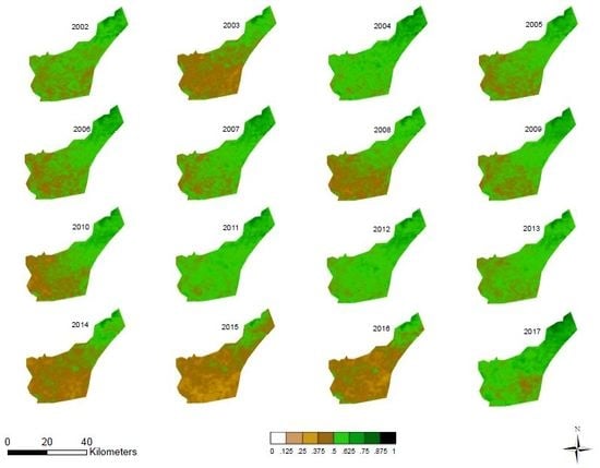
1. Introduction
Vegetation within protected areas such as game reserves provides wildlife and society with indispensable ecosystem goods and services [1] including food, medicinal resources, aesthetic value, and recreational opportunities [2]. However, inappropriate management and other disturbances affect the potential productivity and spatial extent of this resource [3]. Thus, any factor that poses a threat to vegetation and its associated benefits which could affect their productivity in the protected areas needs to be identified and monitored. One such threat is an increase in temperature above normal as well as a prolonged decline in precipitation and soil moisture, leading to extreme climatic events such as droughts, which severely affect vegetation productivity [4]. Drought-related impacts are becoming more multifaceted, as explained by their rapidly growing consequences in sectors such as recreation and tourism, agriculture, and energy [5].
The influence of drought on vegetation varies in the spatial and temporal scales, and these are projected to increase with climate change [6,7]. This behavior affects wildlife, particularly in semi-arid and arid environments where herbivory is strongly restricted by vegetation extent and water availability [8]. In the north-east part of KwaZulu-Natal, South Africa, for example, droughts are becoming a recurrent and prominent feature [9,10], affecting vegetation, water and wildlife resources notably in the Hluhluwe-iMfolozi Park (HiP), the oldest proclaimed game reserve in Africa, as reported in this paper. Furthermore, these impacts have potential consequences that could incapacitate this game reserve’s support of its specialist grazers such as rhinos [11].
Understanding the association between vegetation productivity and climatic variables such as precipitation and temperature has, therefore, become a high priority. To address this, spatiotemporal tools that can integrate climate data with other information of interest are required. Remotely sensed data provide the opportunity to monitor vegetation dynamics in a systematic manner [12]. They play a growing role in drought detection and management as they afford up-to-date information over various time and geographic scales and complement alternative techniques such as field surveys [4] and interviews [13]. Remote sensing’s systematic observation allows us to track vegetation conditions from the 1970s to the present [14] and provides the means to integrate the record with causal factors. This study investigates vegetative drought which is the vegetation stress as a function of moisture deficit [15].
Several drought studies based on satellite-derived measurements have exploited key indicators such as the (a) normalized difference vegetation index (NDVI), a ratio of the difference between the near-infrared and red bands of the spectrum over the sum of the near-infrared and red bands [16,17], which is a robust indicator of vegetation productivity [18]; (b) the normalized difference infrared index (NDII) which contain additional information on water availability in the soil for use by vegetation [19] as measured by the ratios of the near-infrared and short-wave infrared [20]; and (c) the evapotranspiration (ET) which includes both the loss of root zone soil water through transpiration (influenced by stomatal conductance), as well as evaporation from bare soil [21]. These studies have enhanced our understanding of how vegetation reacts to drought events over time [22,23,24,25].
Hitherto, numerous studies have explored vegetation changes using NDVI in response to climatic variability. Most have shown that vegetation is largely swayed by the El Niño/Southern Oscillation (ENSO) phenomenon and have been established to respond well to climatic variables [10,24,26,27]. These studies in different climatic regions have revealed climate-induced effects in key economic sectors such as agriculture [28] and forestry [24,29]. Most recently, Huang et al. [30] used MODIS-derived NDVI to demonstrate how vegetation responds to climate variation in the Ziya-Daqing basins of China. Their results showed that the trends of growing season NDVI were significant in the forest, grassland, and highlands of Taihang but insignificant in most plain drylands [27]. They also showed how grassland, as the primary vegetation on the Qinghai-Tibet Plateau, has been increasingly influenced by water availability due to droughts over the last decade.
Several factors make the HiP an ideal site for assessing the effects of drought on wildlife. First, Bond et al. [31] established that droughts largely influence the extent of grazing vegetation in the reserve. More recently, Xulu et al. [10] showed how the recent intense drought moderated the vegetation health of commercial plantations located ~70 km from the park. Second, the HiP is an important conservation area and ecotourism destination in South Africa [32], so the resultant socio-economic impacts of ecosystem changes are of great concern. In this study, therefore, we aim to evaluate the influence of climatic variability on vegetation in the game reserve over the period of 2002 to 2017. This is the first attempt to demonstrate the spatial dimension of the drought effects in the HiP using satellite data. We show how to construct a MODIS-derived NDVI time series in the GEE platform, and perform statistical tests to determine the causal influence of climatic variables in the reserve.
2. Materials and Methods
2.1. Study Area
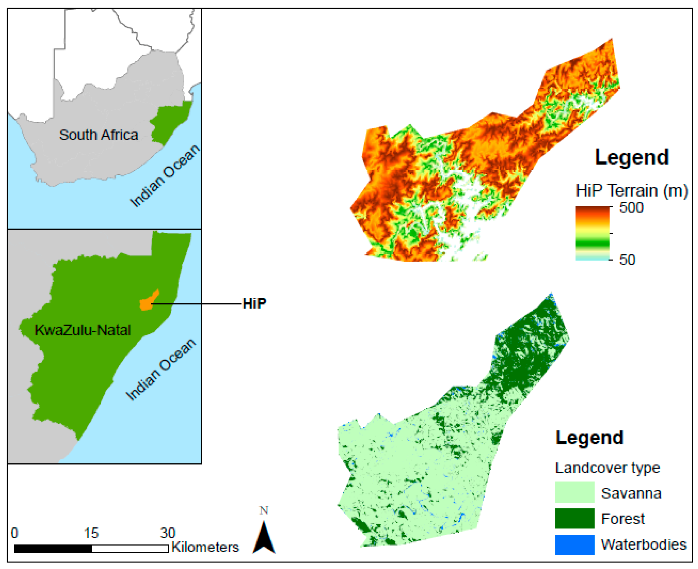
This study was conducted at the Hluhluwe-iMfolozi Park, which covers 900 km2 and extends between 28°00′ S and 28°26′ S, and 31°43′ E and 32°09′ E in the northern KwaZulu-Natal, South Africa (Figure 1). The reserve was established in 1895 and is managed by Ezemvelo KwaZulu-Natal Wildlife (EKZN Wildlife). The landscape undulates with an altitude ranging from approximately 50 to 500 m.a.s.l. and comprises a mixture of soil types resulting from topographic and climatic heterogeneity [33]. The terrain of the study area on the right side of Figure 1 was plotted using the Global Multi-resolution Terrain Elevation Data 2010 data set. The version of this data is the Breakline Emphasis, 7.5 arc-s, and is archived as USGS/GMTED2010 in the Google Earth Engine (GEE) JavaScript platform. Land cover classification was also performed in the GEE environment so as to show the types of vegetation cover in the HiP.
There are two main rivers that pass through this nature park, namely the Black and White Umfolozi. The entire area of the park is fenced and borders on populated rural communities. Vegetation varies from semi-deciduous forests in the north of Hluhluwe to open savanna woodlands in the southern iMfolozi. Much of the area is dominated by woodland savanna interspersed with shrub thicket [34]. The northern part of the park has hilly terrain and is dominated by forest. The climate is subtropical with summer rainfall. It receives a mean annual rainfall ranging from 700 to 985 mm, much of it occurring between October and March [35]. The park supports approximately 1200 plant species, including 300 tree and 150 grass species.
2.2. Data
In order to investigate the variability of vegetation in the HiP in response to climatic conditions as well as the recent intense drought of 2014–2016, we opted to use the monthly averaged MODIS Terra/Aqua 16-day datasets measured for the period from 2002 to 2017 (16 years). With its considerable time resolution (about for images per month) compared to other satellites, MODIS images were the most appropriate for this study because of the size of the geographic area. The MODIS data used here are archived in the GEE as image collection. This data product is generated from a MODIS/MCD43A4 version 6 surface reflectance composite. More details about the MCD43A4 MODIS/Terra and Aqua nadir BRDF-adjusted reflectance daily level 3 global 500 m SIN grid V006 data can be found in a study by Schaaf et al. [36]. The data were extracted and processed using the JavaScript code editor in the GEE platform (https://earthengine.google.com/, Mountain View, CA, USA) (see Appendix A), which provides possibilities of parallel computing and large data processing for even very large study areas. For the purpose of this investigation, our main parameter is the NDVI, but we also considered other vegetation indices such as the Enhanced Vegetation Index (EVI), the Burned Area Index (BAI), and Normalized Difference Infrared Index (NDII). The BAI was also included in order to determine the possible vegetation burning activity, which may have been triggered by drier conditions associated with an intense drought period. NDII has been recently proven to be a robust indicator for monitoring the moisture content in the root-zone from the observed moisture state of vegetation [19,21]. These spectral indices were calculated using the formulas:
where R, NIR, and SWIR1 are spectral bands in the blue (450–500 nm), red (600–700 nm), near-infrared (700–1300 nm), and shortwave infrared (1550–1750 nm) regions.
In this study, we derived the precipitation values averaged for the study area for the period from 2002 to 2017 using the Climate Engine Application (CEA, http://climateengine.org/, Moscow, ID, USA), while soil temperature monthly mean data was derived from the National Aeronautics and Space Administration (NASA, Washington, DC, USA): http://giovanni.gsfc.nasa.gov. Both the soil temperature and precipitation data are an output of the Modern Retrospective Analysis for the Research Application (MERRA-2) model [37]. The MERRA model is an American global reanalysis tool operating from 1979 onwards that is based on the NASA Goddard Earth Observation serving Data Assimilation System version 5 (GEOS-5). The MERRA-2 model data are given at a spatial resolution of 0.67° × 0.50° at 1-hourly to 6-hourly intervals.
There is always an expected variability of surface water content due to changes in both weather and climatic conditions. Therefore, in a study such as this one, it is essential to always investigate the water lost to the atmosphere through both evaporation and transpiration. This can be an important process as it could explain details about vegetation water stress. Given that the study area is a remote area which does not have evaporation and/transpiration measurements records, we opted to use the Global Land Data Assimilation System (GLDAS) evapotranspiration (ET) data. The GLDAS system was designed to generate optimal fields of land surface and fluxes, and it is also capable of generating quality controlled, spatially and temporally consistent, terrestrial hydrological data including ET and other related parameters [38].
The ENSO phenomenon influences rainfall and temperature conditions largely over southern Africa [39,40]. Previous studies have demonstrated how vegetation responds significantly to ENSO [40] and the DMI [41] index as a measure of climatic conditions [42,43,44] in some parts of southern Africa. Thus, in order to investigate changes in vegetation in the HiP due to variability in climatic conditions, it is important to consider these climate indices. In this study, we used the Niño3.4 monthly mean time series retrieved from the National Oceanic and Atmospheric Administration (NOAA) website (https://www.esrl.noaa.gov/psd/gcos_wgsp/Timeseries/, Washington, DC, USA). The Niño3.4 index is calculated by taking the area-averaged sea-surface temperature (SST) within the Niño3.4 region, which is at 5° N–5° S longitude and 120° W–170° W latitude in the Pacific Ocean. On the other hand, the DMI is calculated by taking the difference between the SST anomalies in the western (50° E–70° E; 10° S–10° N) and eastern (90° E–110° E), (10° S–0° N) sectors of the equatorial Indian Ocean [41]. The DMI data were downloaded from the website: http://www.jamstec.go.jp/frcgc/research/d1/iod/iod/dipole_mode_index.html. The relevant time series of Niño3.4 and DMI are shown in Figure 2.
2.3. Multiple-Linear Regression
One of the principal objectives of this study is to quantify the effects of temperature, precipitation, ET, soil moisture at root-zone (NDII), ENSO and DMI on the NDVI as a surrogate for vegetation in the study area. Multiple-linear regression analysis (MLR), which is commonly used to explain the relationship between one continuous dependent variable and two or more independent variables, was employed. The MLR model output of a number n observations can be represented as
where yi is the dependent variable (NDVI in this case), xip represents the independent variables (soil temperature, precipitation, Niño3.4, and DMI in this case), β0 is the intercept, and β1, β2, … βp are the coefficients of the x terms. The term εi represents the error term, which the model always tries to minimize.
2.4. Mann–Kendall Test
It is always useful to assess the monotonic trends in a time series of any geophysical data. In this study, the Mann–Kendall test [45,46,47] was used. This is a non-parametric rank-based test method, which is commonly used to identify monotonic trends in a time series of climate data, environmental data, or hydrological data. Non-parametric methods are known to be resilient to outliers [48], hence it is desirable to choose such methods. Based on a study by Kendall [47] and recently by Pohlert [49] and others, the Mann–Kendall test statistic is calculated from the following formula:
where
The average value of S is E[S] = 0, and the variance σ2 is given by the following equation:
where tj is the number of data points in the jth tied group, and p is the number of the tied group in the time series. It is important to mention that the summation operator in the above equation is applied only in the case of tied groups in the time series in order to reduce the influence of individual values in tied groups in the ranked statistics. On the assumption of random and independent time series, the statistic S is approximately normally distributed provided that the following z-transformation equation is used:
The value of the S statistic is associated with the Kendall
where
In regards to the z-transformation equation defined above, this study considered a 5% confidence level, where the null hypothesis of no trend was rejected if |z| > 1.96. Another important output of the Mann–Kendall statistic is the Kendall τ term, which is a measure of correlation which indicates the strength of the relationship between any two independent variables. In this study, the Mann–Kendall test system summarized above was applied to the NDVI data by writing a piece of code in R-project and following the instructions by Pohlert [49].
The Mann–Kendall trend method can be extended into a sequential version of the Mann–Kendall test statistic which is called the Sequential Mann–Kendall (SQ-MK). This method was proposed by Reference [50], and it is used to detect approximate potential trends turning points in long-term time series. This test method generates two time series, a forward/progressive one () and a backward/retrograde one (). In order to utilize the effectiveness of this trend detection method, it is required that both the progressive and the retrograde time series are plotted in the same figure. If they happen to cross each other and diverge beyond the specific threshold (±1.96 in this study), then there is a statistically significant trend. The region where they cross each other indicates the time period where the trend turning point begins [51]. Basically, this method is computed by using ranked values of of a given time series () in the analyses. The magnitudes of n) are compared with j − 1). At each comparison, the number of cases where are counted and then donated to . The statistic is thereafter defined by the following equation:
The mean and variance of the statistic are given by
and
Finally, the sequential values of statistic which are standardized are calculated using the following equation:
The above equation gives a forward sequential statistic which is normally called the progressive statistic. In order to calculate the backward/retrograde statistic values (), the same time series ) is used, but statistic values are computed by starting from the end of the time series. The combination of the forward and backward sequential statistic allows for the detection of the approximate beginning of a developing trend. Additionally, in this study, a 95% confidence level was considered, which means critical limit values are ±1.96. This method has been successfully utilized in studies of trends detection in temperature [52,53] and precipitation [51,53,54].
2.5. Wavelet Transforms and Wavelet Coherence
In this study, we opted to employ the wavelet transform analyses method [55] because of its ability to obtain a time–frequency representation of any continuous signal. Basically, the continuous wavelet transform (CWT) of a given geophysical (in this case) time series is given by transforming the time series into a time and frequency space. While there are several types of wavelets, the choice of the wavelet function is determined by the data series, of which, for geophysical data, the Morlet wavelet function has been shown to perform well [55,56,57]. Thus, the CWT [Wn (s)] for a given time series (xn, n = 1, 2, 3, …, N) with respect to wavelet Ψ0 (η) is defined as:
where s is the wavelet scale, n′ is the translated time index, n is the localized time index, and Ψ* is the complex conjugate of the normalized wavelet. δt is the uniform time step (which is months in this case). The wavelet power is calculated from |Wn (n)|2. In this study, the CWT statistical significance at a 95% confidence level was estimated against a red noise model [55,57]. Using a continuous wavelet transform analysis, it is also possible to quantify the relationship between two independent time series of the same time step δt. In this study, the aim was to quantify the relationship between NDVI averaged for the study area and selected climatic parameters. Following Grinsted et al. [57], for the two time series of X and Y, with different CWT and values, the cross-wavelet transform is given by
where “*” represents the complex conjugate of the Y time series. The output of the above equation can also assist in calculating the wavelet coherence. Basically, wavelet coherence is a measure of the intensity of the covariance of the two time series in a time–frequency domain. This is an important parameter because the cross-wavelet only gives a common power. Another important process is to calculate the phase difference between the two time series. Here, the procedure is to estimate the mean and confidence interval of the phase difference. Following a study by Grinsted et al. [57], we used the circular mean of the phase-over regions with relatively high statistical significance that are inside the cone of influence (COI) to quantify the phase relationship between any two independent time series. As defined in a study by Zar [58] and also later by Grinsted et al. [57], the mean circulation of a set of angles (ai, i = 1, 2, 3,…, n) can be defined by the following equation:
Following the studies by Torrence et al. [55,57], the wavelet coherence between two independent time series can be calculated using the following equation:
where the parameter S is the smoothing operator defined by S(Wn (s)) = Sscale (Stime (Wn(s))). The parameter Stime represents the smoothing in time. For further details about the theory of wavelet analyses, the reader is referred to [55,57,59].
3. Results and Discussion
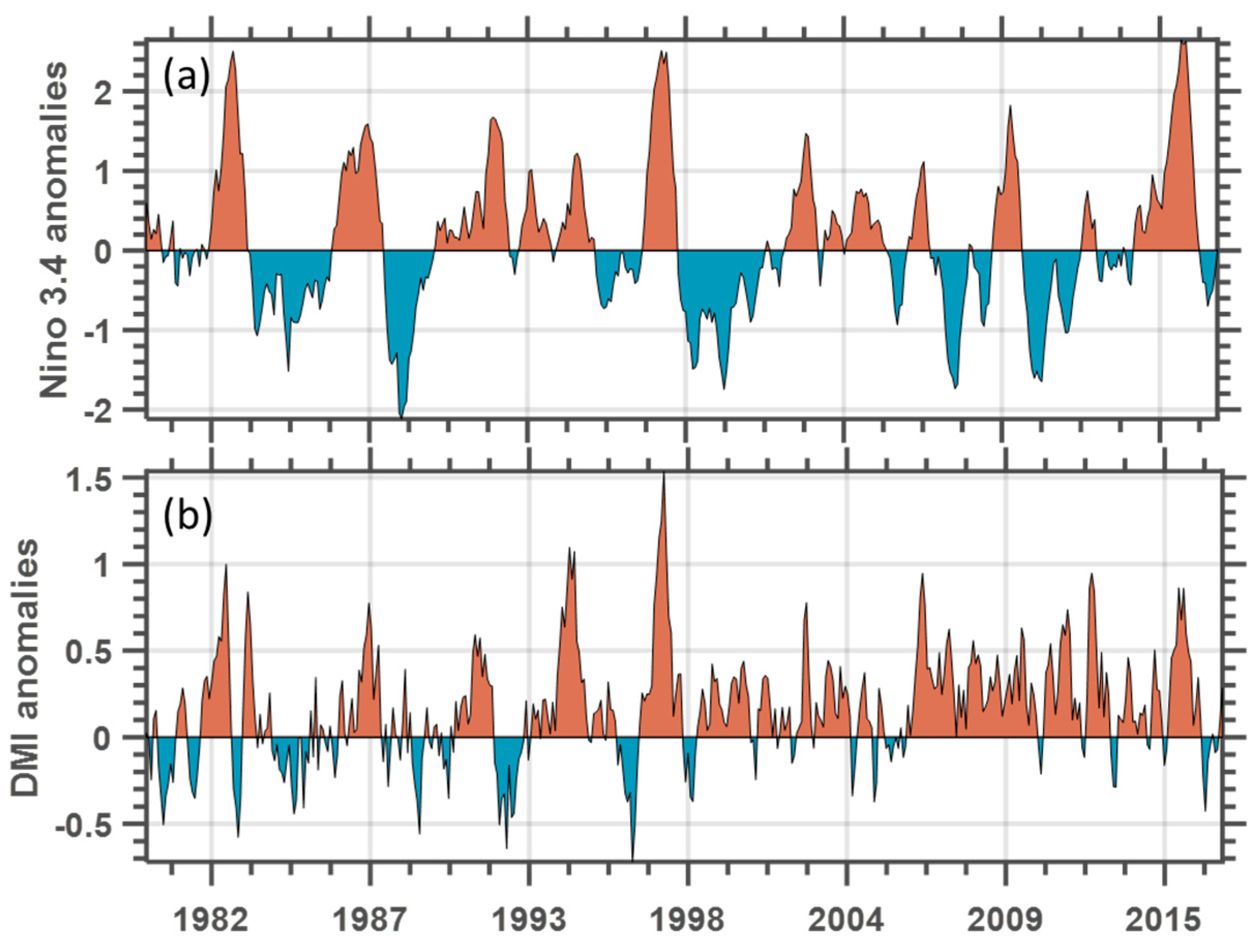
To investigate whether the El Niño event of 2014–2016 can be classified as a strong El Niño event, a time series for the period from the beginning of the satellite era (1980) to 2017 was plotted (see Figure 2a). We also considered the DMI index (Figure 2b) as a measure of climatic conditions of the eastern part of southern Africa [43]. A general classification of ENSO events should contain 5 consecutive overlapping 3-month periods with SST anomalies below −0.5 for the La Niña events and above +0.5 for the El Niño events.
In Figure 2a,b, both the El Niño events and positive DMI are shaded in red, whereas La Niña and negative DMI are indicated in blue. To identify the strength of the ENSO events, the threshold is further broken down to weak (0.5–0.9 SST anomaly), moderate (1.0–1.4 anomaly), and strong (≥1.5 anomaly) events. Figure 2a shows that the 2014–2016 El Niño was one of the strongest since the beginning of the record. Other notably strong El Niño occurrences were in 1982/1983, 1997/1998, and 2009/2010. On the other hand, there were many episodes of positive DMI, with one such event in the 2014–2016 period, which seems to be in phase with the recent strong El Niño of 2014–2016.
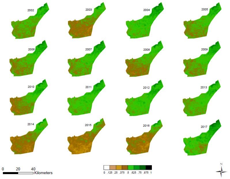
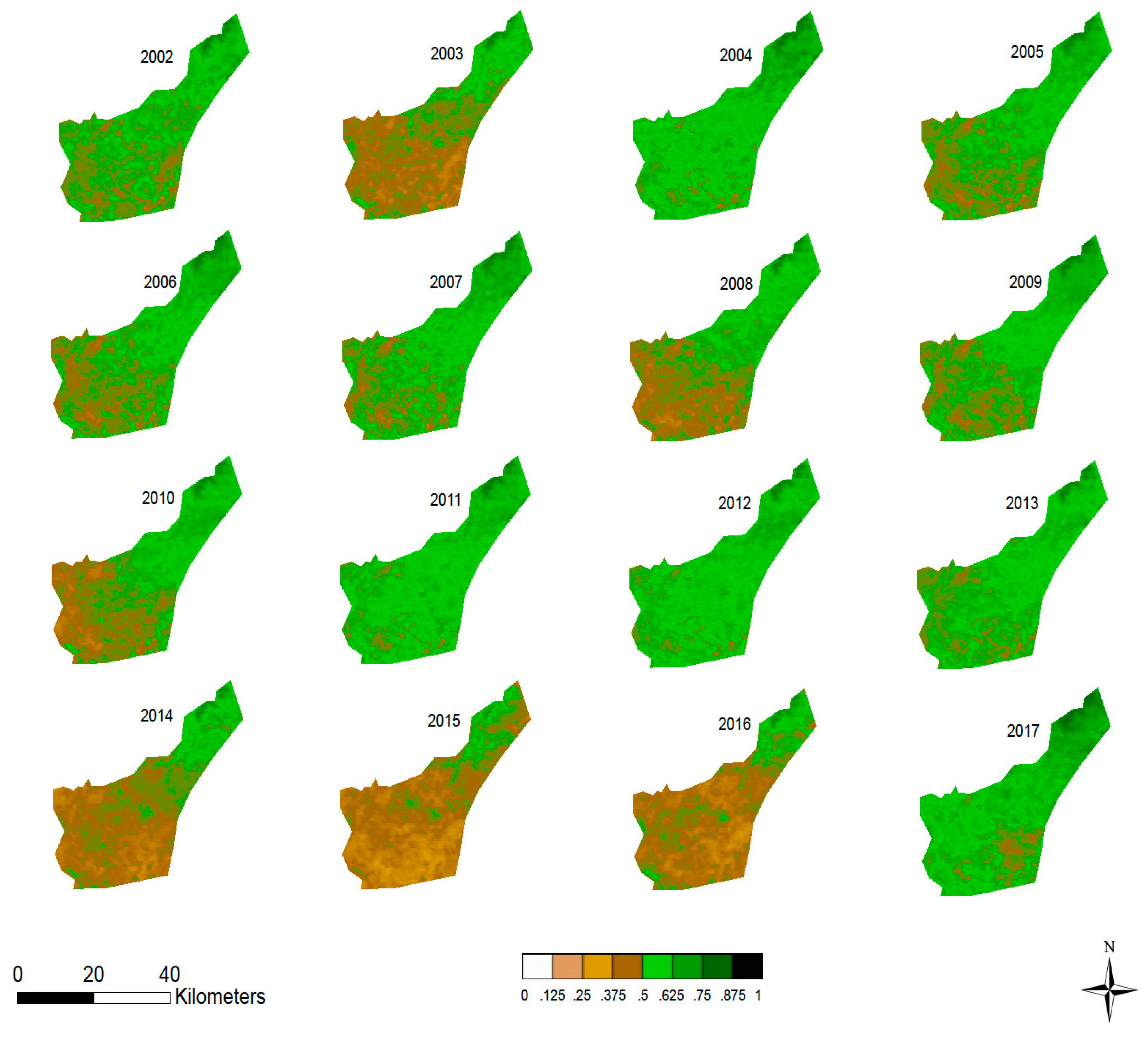
A composite of the NDVI index averaged for each year from 2002 to 2017 is shown in Figure 3. In this figure, regions where there are greener colors indicate higher NDVI values, whereas the brownish colors indicate low NDVI values. These results show that there seems to be a direct influence of the ENSO in the vegetation of the HiP, especially during strong El Niño years (2014–2016). It is evident that during El Niño years, there was a decline in NDVI values especially in the southern and western parts of the study area. This is presumably because the vegetation of the northern part of the HiP is dominated by a forest which is consist of indigenous trees which are believed to be drought resistant (see Figure 1). Additionally, the contributing factor could be that the eastern part of the HiP is benefiting from orographic lifting as it is situated in a high terrain (see Figure 1). The evidence of the influence of El Niño is more prominent during the strong El Niño years such as 2003 and the recent intense 2014–2016 drought period, as well as the 2008 non-ENSO drought period.
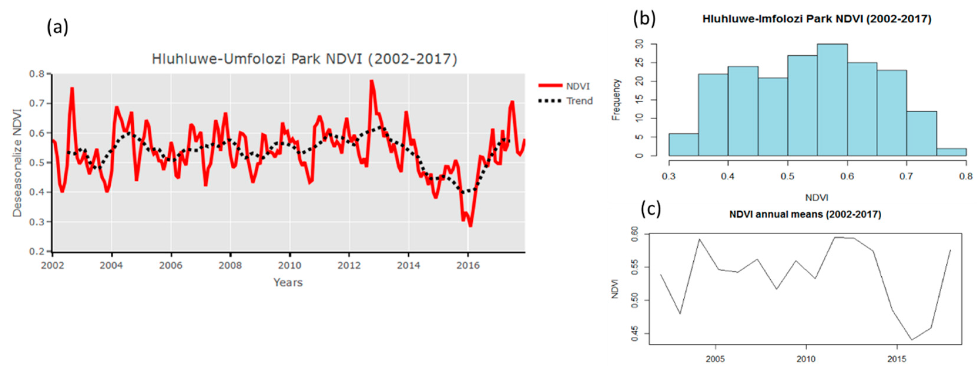
Figure 4a shows the deseasonalized monthly averaged MODIS NDVI time series for HiP from 2002 to 2017 (red line) plotted together with the 12 months running mean smooth trend (black dotted line). The monthly mean NDVI values plotted in Figure 4a were calculated by taking an averaged of MODIS images available in that month. In this study area, the MODIS satellite records four images per month. In general, there is a steady trend of NDVI measured at the HiP beside some anomalies observed in specific parts of the time series. This seems to be the case for southern Africa because other studies also indicated a steady trend for this region [10]. Remarkably, during the 2014–2016 period, a period that coincided with the recent intense El Niño, there was a sudden decrease in the NDVI values which reduced to the lowest minimum value of about 0.3 in November 2015. During this period, EVI values also decreased to minimum values of about 0.11 (results not shown here).
A study by Mberego and Gwenzi [60] investigated the temporal patterns of precipitation and vegetation variability over Zimbabwe during extreme dry and wet rainfall seasons using data covering the period 1981–2005. Their NDVI time series indicated a steady trend over this period. However, it seemed to be strongly affected by severe dry conditions, an observation which is consistent with the results presented here. In this study, the deseasonalized monthly mean NDVI time series in Figure 4a (red line) indicates the possible response that corresponds to both dry and wet years, especially during the most recent strong El Niño events of 2003 and 2014–2016. In relation to the strength of the influence of El Niño in the south-western part of southern Africa, a study by Manatsa et al. [61] analyzed agricultural drought in Zimbabwe using the standardized precipitation index (SPI). They reported the 1991–1992 period as the period which experienced the most extreme drought conditions. A little later, observations by Mberego and Gwenzi [60] reported the year 2002–2003 as the drought period with the most prolonged time of relatively low NDVI values in their time series. While our study does indicate a significant influence of the 2003 El Niño event in the HiP NDVI values, the observations presented here indicate that 2014–2016 was the longest period with low NDVI values. Thus, 2014–2016 could be regarded as the most recent intense El Niño period, with a maximum effect on vegetation in the HiP. The NDVI values dropped from a value ~0.65 in November 2013 to 0.3 in November 2015. This is also verified by a much smoother representation of the NDVI in Figure 4c in which a reduction in NDVI values is observed. This reduction coincides with the most recent strong El Niño. Additionally, a reduction which coincides with the El Niño of 2003 (see Figure 4c). Another significant feature is a strong peak, which reaches ~0.8 just after the Irina tropical storm, which occurred in early March 2012 (see Figure 4).
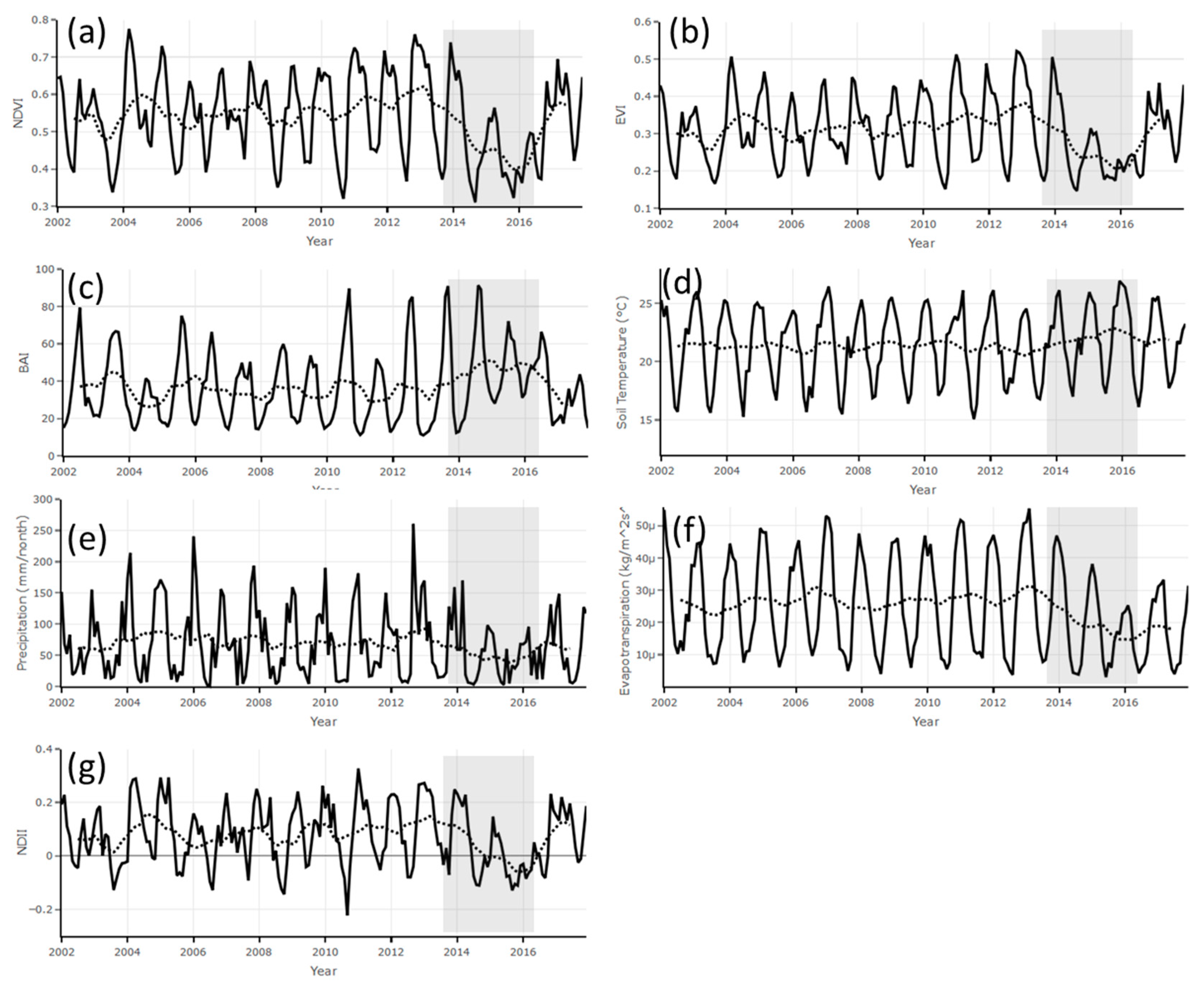
Figure 5 shows monthly mean time series values plotted together with their corresponding 12-month running-mean smooth trend for NDVI (Figure 5a), EVI (Figure 5b), BAI (Figure 5c), soil temperature (Figure 5d), precipitation (Figure 5e), evapotranspiration (Figure 5f), and NDII (Figure 5g). These monthly mean values are plotted together with their respective smooth trends, which were calculated using the Breaks For Additive Season and Trend (BFAST) method, which is described in details by Verbesselt et al. [62,63]. Basically, the BFAST method integrates the decomposition of time series seasonal, trend, and remainder components of any satellite image time series, and can be applied to any other type of time series in the geosciences that deals with seasonal or non-seasonal time series. The period of the most recent intense drought (2014–2016) is indicated by the grey shaded box in each figure. In general, all the parameters show a seasonal cycle in terms of monthly means.
There is an expected resemblance between the NDVI and EVI observations in both the monthly mean time series and the smooth trend, with a clear indication of the effect of the 2014–2016 drought period. These observations are consistent with a study by Xulu et al. [10], who investigated the response of commercial forestry to the recent strong and broad El Niño event in a region which is 70 km south-east of the HiP. In their study, Xulu et al. [10] reported a significant decline of NDVI values which corresponded to the 2014–2016 El Niño years [10]. Although the influence of the 2014–2016 El Niño in the HiP seems to be the strongest, it follows the same pattern as that reported by Anyamba et al. [40] in their study of the influence of both El Niño and La Niña in the vegetation status over eastern and southern Africa. Considering the level of browning of vegetation demonstrated in Figure 3 for the years 2014–2016, it is necessary to consider the possible fire activity given the relatively dry conditions in the HiP. Figure 5c indicates that during the period of the intense drought of 2014–2016 there was an increase in fire incidences in the HiP. This is revealed by a rise in the BAI values of the smooth trend to its maximum level of approximately 50 in November 2015. During the 2014–2016 period, the HiP experienced an unprecedented decline in the total precipitation per month (see Figure 5d). During the same period, the soil temperature increased to its highest maximum (see Figure 5e). The GLDAS monthly mean ET time series shown in Figure 5f indicates a declining trend during the period 2014–2016, which indicated a possible vegetation stress. In order to investigate the moisture content at root-zone, the NDII index was used. The NDII (Figure 5g) indicates a similar pattern to that of the NDVI and EVI time series. It is observed in Figure 5a that the NDII had a steady trend (0.10) during the period 2002–2013 which was followed by a sudden decrease which reached a minimum value of −0.06 in November 2015.
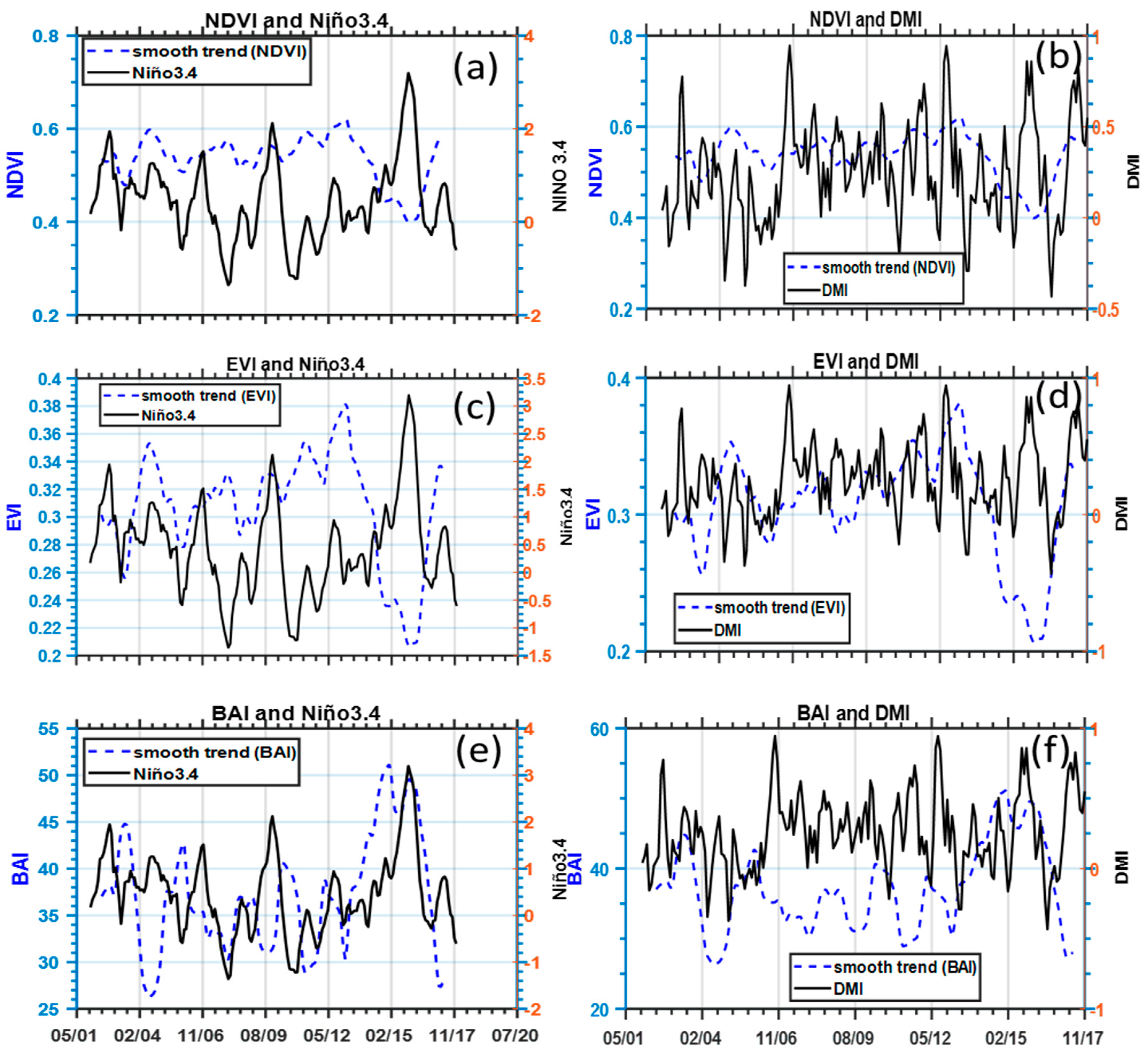
The 12-month running mean smooth trends extracted using the BFAST method for NDVI, EVI, and BAI plotted against anomalies of climatic forcers Niño3.4 and DMI are shown in Figure 6. This plot was constructed to investigate any possible 2-dimensional teleconnection between vegetation condition and the Niño3.4 and DMI climatic forcers, respectively. The panels on the left represent the vegetation indices versus Niño3.4, and the panels on the right show the vegetation indices versus DMI. Both the NDVI (Figure 6a) and EVI (Figure 6b) values show a fairly steady pattern for most parts of the time series, which vary between NDVI values of 0.50 and 0.60, and between EVI values of 0.28 and 0.34. However, both the NDVI and EVI values seem to be enhanced by the extreme amount of rainfall that was brought by the tropical cyclone Irina during early 2012 in the eastern part of southern Africa. In that year, NDVI values increased to a maximum value of approximately 0.62, whereas the more sensitive EVI index reached its maximum of approximately 0.38. The strong peaks that were observed during 2004 for both the NDVI and EVI time series correspond to the greening of vegetation in the HiP which was produced by heavy rainfall that was brought by tropical cyclone Elite in January 2004 [64]. NDVI values were observed to decrease sharply from late 2013 until they reached their minimum of approximately 0.40 in 2015 before beginning to recover to normal average conditions in 2017. This pattern is also depicted in the EVI time series and is directly linked to the stronger and more extensive 2014–2016 El Niño event. Similar results were also presented in a study by Xulu et al. [10], who investigated the influence of recent droughts on forest plantations in Zululand. The notable browning observed in Figure 3 for years 2014, 2015 and 2016, which was also revealed by the NDVI and EVI time series (Figure 5), seems to represent favorable conditions for biomass burning in the HiP. This is revealed by the unprecedented sudden increase of BAI values to its highest maximum of approximately 50, which coincides with the enhancement of Niño3.4 during 2014–2016 (Figure 6e).
The DMI was highly variable compared to the Niño3.4 climatic forcer throughout the study period, with several distinctive positive DMI values that reached a maximum of just below 1.0. Remarkably, there is a strong peak that extends up to approximately 0.8 during the period band corresponding to 2014–2016 that coincided with the decline in NDVI and EVI and the increase of the ENSO and BAI time series. We note here that the widespread browning observed during the 2014–2016 drought period could have been accelerated by the fact that the climatic forcers, which are known to influence the south-eastern part of southern Africa, may have been in phase during this period. This, of course, needs further investigation; and is discussed below.
3.1. Correlations Statistics and Mann–Kendall Test
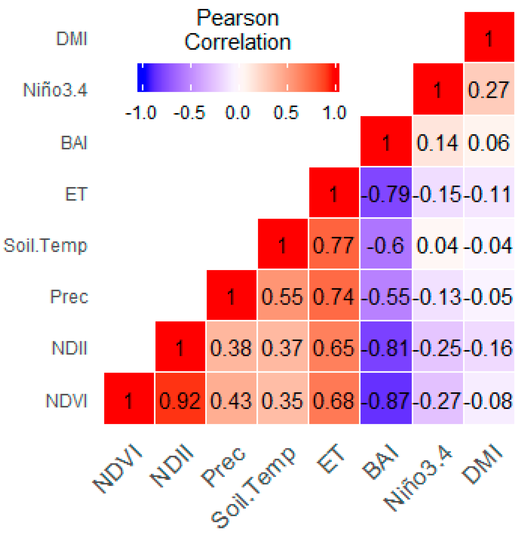
The Pearson correlation between NDVI and climatic variables used in this study for the whole study record was derived. Figure 7 shows the heat map which summarizes the linear relationships between all the parameters monitored in this study. In this figure, it is clear that there is a strong correlation between NDVI and Soil temperature (r = 0.35), precipitation (r = 0.43), ET (r = 0.68), and NDII (r = 0.92). On the other hand, there is a significance strong negative correlation between the NDVI and BAI, which is not surprising because greener vegetation reduces chances of biomass burning, while the possibility of the satellite detecting a charcoal signal from burnt vegetation during dry conditions is high. There is also a noteworthy negative (r = −0.27) correlation between NDVI and Niño3.4. The results shown in Figure 7 also reaffirm the strong relationship between soil temperature with a strong correlation coefficient of r = 0.77. Considering that Figure 2 indicates some episodes where a strong Niño3.4 peak is in phase with the DMI peaks, the noteworthy correlation of r = 0.28 between these two climatic indices seems to reaffirm this.
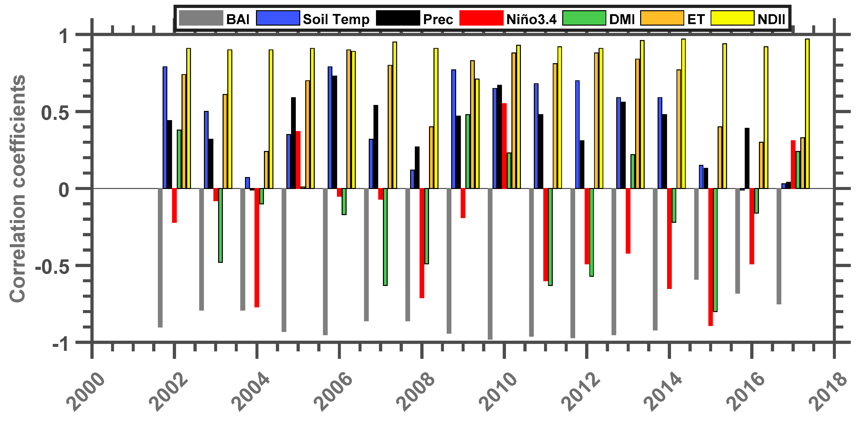
Figure 8 shows the inter-annual variability of the Pearson linear correlation between the HiP NDVI values and parameters such as BAI, Soil Temp, Prec, Niño3.4, DMI, ET, and NDII for the period from 2002 to 2017. The correlation between NDVI and EVI was not analyzed because the two parameters closely resemble each other. In general, NDVI is positively correlated to soil temperature, precipitation, ET and NDII through the study period. The NDVI–NDII correlation was the strongest positive correlation with an average value of r = 0.91. This reaffirms the strong relationship between vegetation water stress and soil moisture at the root-zone. The NDVI–ET correlation was observed to be steady at an average correlation coefficient value of r = 0.65 during the period from 2002–2013. However, this linear relationship decreased to r = 0.40 and r = 0.30 in 2015 and 2016, respectively. A study by [65] also used MODIS NDVI and GILDAS evapotranspiration data in order to investigate the relationship between NDVI and evapotranspiration. In their study, they reported a steady positive inter-annual variability of correlation coefficients with an average value of r = 0.58. As expected, the NDVI–Niño3.4 correlation is dominated by negative values which are observed to decrease during the periods corresponding to El Niño years. This is consistent with previous studies such as those of Xulu et al. [10,40] who reported a significant influence of ENSO on the vegetation of southern Africa, especially the north-eastern part. Moreover, a salient observation is that the greatest minimum correlation recorded was in 2015, a year with a particularly strong El Niño. The negative correlation between DMI and NDVI also seems to be greater during the recent intense drought period, which could indicate that Niño3.4 and DMI were in phase during this time. The correlation between NDVI and the BAI is expected to be strongly negative as greening is not conducive to biomass burning. However, the results presented in Figure 8 indicate that there was a sudden increase in correlation between NDVI and BAI in 2015 before it returned to its average position in 2016 and 2017. Overall, the inter-annual variation of almost all the study parameters indicates a noticeable change during El Niño events in the years 2003 and more prominently during the 2014–2016 period.
A comprehensive summary of the MLR analysis statistics encompassing NDVI, temperature, precipitation, Niño3.4, and DMI is shown in Table 1. It should be mentioned that the soil temperature, precipitation, ET, NDII, and Niño3.4 were used in this model because of their well-known possible influence on NDVI variability. The DMI climatic parameter was not used as an explanatory variable in the MLR model because of its weak correlation with the NDVI. The results in Table 1 reveal a statistically significant relationship between NDVI and soil temperature and between NDII and ET, with p-values of 0.000386, <2.00 × 10⁻¹⁶ and 0.000173, respectively. Both Precipitation and Niño3.4 indicate a statistically insignificant association with the NDVI because of p-values which are far greater than 0.05. A positive significant correlation between NDVI and Soil temperature, NDII, and ET, which is also represented as in Figure 7 and Figure 8, indicates that soil moisture, soil temperature, and evapotranspiration play a significant role in vegetation health in the HiP. The significant but negative correlation between Niño3.4 and NDVI confirms the notion that ENSO variability plays a role in the climatic conditions of southern Africa [35,52].
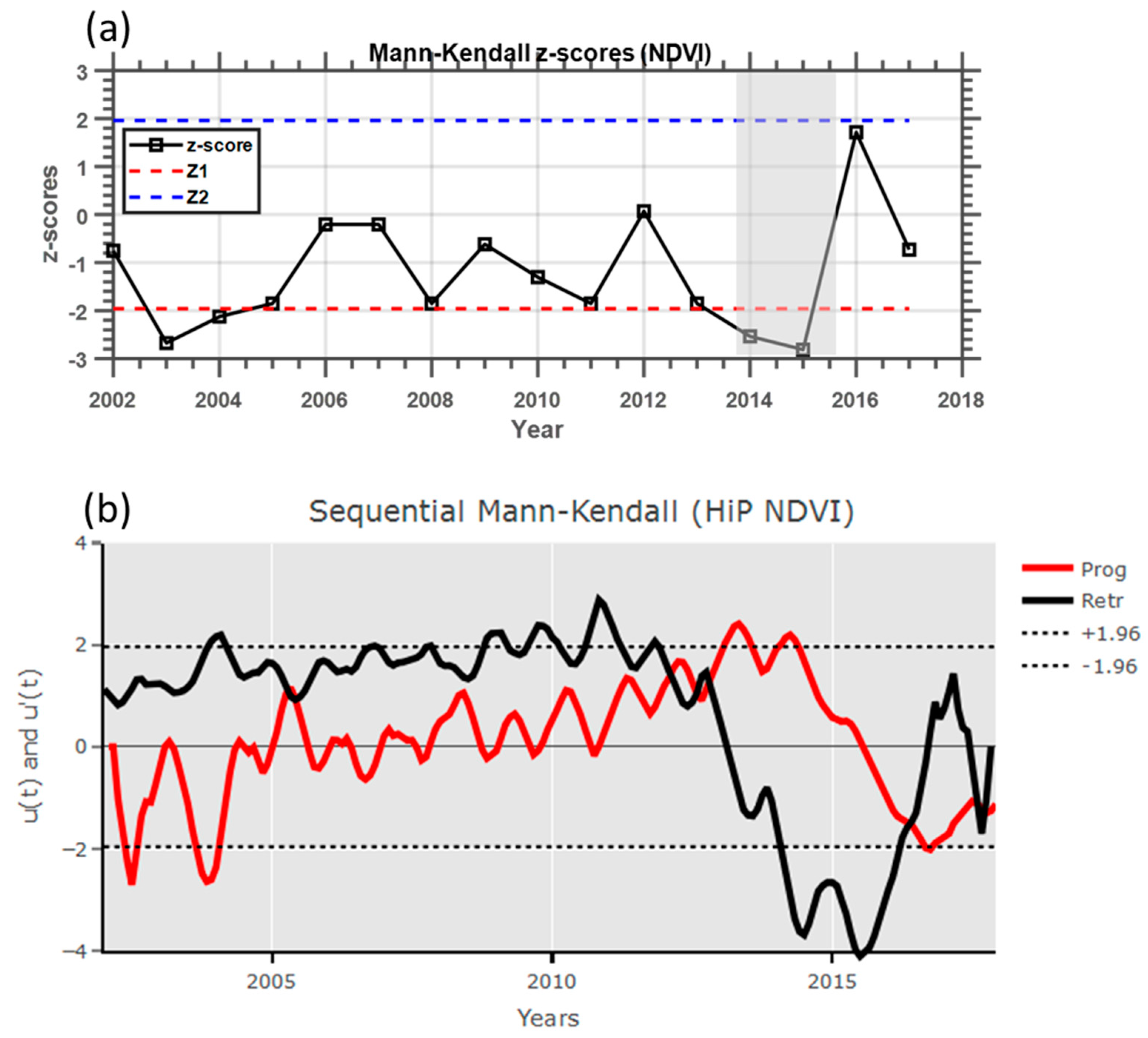
In this study, the Mann–Kendall trend test was used for the analysis of the trend in the HiP NDVI time series. The main advantage of this technique is that it provides a non-parametric test that does not require data to be normally distributed, and it is not dependent on the magnitude of data. Furthermore, this non-parametric test method has a low sensitivity to abrupt breaks in heterogeneous time series [66]. The Mann–Kendall test model was applied to the NDVI data, and the results are shown in Figure 9. In summary, the z-score and p-value for the entire NDVI time series period (2002–2017) were found to be −1.22 and 0.224, respectively. Both the z-score and the p-value seem to indicate that there was a downward but not significant trend in the NDVI data. The indication of an insignificant downward trend (negative z-score) presumably due to the unprecedented sudden reduction of the NDVI values which coincided with the 2014–2016 drought. In order to investigate the influence of drought conditions in the study area using the Mann–Kendall method, it is necessary to calculate the inter-annual variation of Mann–Kendall z-scores. These Mann–Kendall z-scores were calculated from monthly means for each year starting from 2002–2017.
Figure 9a shows the Mann–Kendall z-scores based on the 16 years of monthly average NDVI data for the game reserve. In general, it is expected that vegetation will respond to climate fluctuating conditions, and this is clearly depicted by significantly negative z-scores (less than Z1 = −1.96) during strong El Niño events (e.g., in 2003 and 2014/2015). The significant downward trend observed between 2014 to 2015 is the strongest such downward trend in the history of the MODIS NDVI data used in this study; it demonstrates a clear response of the vegetation of the reserve to the strong El Niño event of 2014–2016. Similar analysis and results comparable with those presented here were reported by Hou et al. [24] in their study on the inter-annual variability in growing-season NDVI and its correlation with climate variables in the south-western Karst region of China.
The sequential version of the Mann–Kendall test was applied to the NDVI monthly mean time series so as to determine the approximates time periods of the beginning of a significant trend. Figure 9b shows the sequential statistic values of forward/progressive (Prog) (solid red line) and retrograde (Retr) (black solid line) obtained by SQ-MK test for HiP monthly mean NDVI data for the period from 2002 to 2017. There is a noticeable statistically significant downward trend which seems to coincide with the 2003 and strongly the 2014–2016 strong El Niño event. These independent calculations are in agreement with the inter-annual variation of the Mann–Kendall z-scores results presented in Figure 9a. In the case that seems to be associated with the 2014–2016 strong El Niño events, there is an apparent downward trend (indicated by the retrograde) that begins in November 2012 and reaches the negative significant trend limit (−1.96) in April 2014. The retrograde statistic values stay in significant negative territories during the period from April 2014 to May 2016 before it starts to revert back to be within the 95% confidence level limits (±1.96). This trend is regarded as significant because the progressive and retrograde curves intersect each other (turning point) within the limits of the 95% confidence level. This significant trend turning point took place during November 2012. Another significant downward trend was observed in late 2003, with the significant trend turning point observed in June 2005.
The intensity of the 2014–2016 drought impact in the HiP has been identified to be identical to that of the early 1980s [11]. Some of the additional factors that reportedly intensified the impact of the 2014–2016 drought include the reduction in the grazing lawns, siltation of rivers, and the increasing number of carnivores [11]. The impact of the 2014–2016 drought did not only affect this natural protected area (HiP), but also the comical plantations which are situated at about 70 km southwest of the HiP [10], [67]. A study by Crous et al. [67] reported a large-scale dieback of Eucalyptus grandis × E. urophylla (SClone) in the Zululand coastal plain, KwaZulu-Natal, South Africa, during the recent intense drought. This was later supported by Xulu at al. [10], where they reported that the commercial forest of kwaMbonambi, northern Zululand suffered drought stress during 2015.
3.2. Wavelet Analyses
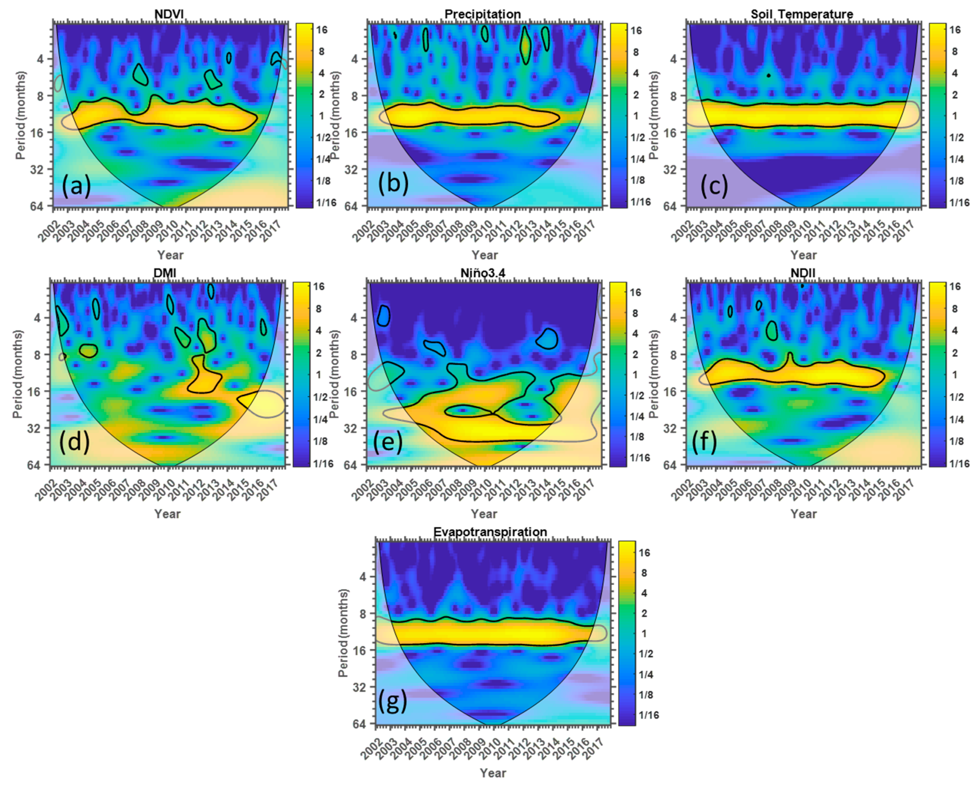
In order to analyze the localized variation of the spectral power within the time series, wavelet analyses, the most common tool for this purpose, was conducted. As mentioned earlier, the wavelet method assists by decomposing a time series into a time–frequency space, which makes it possible to determine the dominant modes of variability and how they vary in time. Figure 10 shows the normalized wavelet power spectra for the monthly mean NDVI, precipitation, soil temperature, DMI, Niño.3.4 NDII, and ET data. The results of the EVI wavelet analyses are not shown here because this time series is identical to that of the NDVI. In Figure 10, the blue color indicates low wavelet power, and the yellow color represents areas of high wavelet power. The horizontal axis is the time scale (in years) and the vertical axis is the period (in months). The thick black line represents the 95% confidence level. The areas of the wavelet power that are considered are those which are within the cone-of-influence (indicated by the solid “u” shaped line). The con-of-influence indicates areas where edge effects occur in the coherence data [55,57].
The NDVI of the HiP seems to follow the distinctive pattern of the seasonality of precipitation in the north-eastern part of South Africa. The region experiences rainfall during the summer period (December–February) and dry winter period (June–August). This is confirmed by a statistically significant peak observed at around the 12-month cycle (see Figure 10a), which seems to correspond with that of precipitation (Figure 10b). The wavelet power spectra of soil temperature (Figure 10c), NDII (Figure 10f) and ET (Figure 10g) also indicate a strong peak at around the 12-month cycle. This is plausible because wet seasons (summer in this case) lead to increased soil moisture and also create conditions of low evapotranspiration and thus accelerate the greening process in the HiP. It should also be noted that the NDVI wavelet power spectra have significant peaks showing the presence of the semi-annual oscillation (6 months), which is observed during the distinctive period from 2006–2007 to 2011–2012. The semi-annual oscillation observed during the 2006–2007 period is also apparent in the NDII wavelet power spectra. The results of the NDVI wavelet spectral presented here are remarkably similar to the findings of Azzali and Menenti [12], who used a Fourier transform-based technique and reported a substantial seasonal change in NDVI for southern Africa. The significant power of a period of 3–4 months that is observed during the distinctive period 2012–2013 and 2015–2016 in the precipitation power spectra is perhaps related to cyclone Irina in early 2012 and the most recent intense drought of 2014–2016. The wavelet power spectra of the DMI indicate a significant power peak of distinctive periods in the 3–20 months band primarily during the period between 2008 and 2013. On the other hand, the Niño3.4 power spectra exhibit significant power peaks in the 8–32 months band throughout the study period. It should be noted, however, that this frequency of occurrence of peaks observed in the Niño3.4 wavelet spectra is similar to that reported in the studies of Torrance and Compo [55] and also of Jevrejeva et al. [56], who used a much longer time series of the ENSO signal.
The wavelet coherence between NDVI–Niño3.4, NDVI–DMI, NDVI–precipitation, NDVI–soil temperature, NDVI–NDII, and NDVI–ET was investigated to determine whether NDVI significant wavelet spectra peaks observed at a given time correspond with those observed by the other parameters. Furthermore, the phase relationship between NDVI and the other parameters was calculated and superimposed graphically in Figure 11. The phase relationship is represented by arrows, where two cross-wavelet parameters are in phase if the arrows point to the right, anti-phase if the arrows point to the left, and NDVI leading or lagging if the arrows point upwards or downwards, respectively. The vectors were only plotted for areas where the squared coherence is greater or equal to 0.5. More details about these calculations can be found in References [56,57] and later by studies by Schulte et al. [59].
The local wavelet coherence spectra together with their distinctive cross-spectra phase for NDVI–Niño3.4, NDVI–DMI, NDVI-precipitation, NDVI–soil temperature, NDVI–NDII, and NDVI–ET are shown in Figure 11. In general, all the wavelet coherence spectra indicate that Niño3.4, DMI, precipitation, soil temperature, NDII, and ET do have some degree of coherence with the HiP NDVI in a variety of both periods and timescales. However, it should be mentioned that because statistically, the significant correlation between any two variables being investigated could occur by chance, a significant commonality in a wavelet coherence spectra analysis does not necessarily imply interconnection. Moreover, there is a possibility of smaller areas of wavelet coherence occurring by chance, which would not indicate interconnection, whereas larger areas of significance are improbable due to chance. For this reason, further investigation is required in regard to a possible teleconnection between any two-time series.
A study by Torrance and Compo [55] investigated the periodicities present in a much longer time series (1871–1996) of Niño3.4 using Morlet wavelets and reported the domination of periods greater than 12 months, with some episodes of shorter periods also present in their spectra. In this study, the wavelet coherence between NDVI and Niño3.4 indicates smaller or no areas of high power significance, which is understandable because the 16-year monthly mean NDVI time series is dominated by periodicities of less than 16 months (Figure 10a) whereas the Niño3.4 wavelet spectra are dominated by periodicities greater than 12 months. Remarkably, there is a significant power at a period band of 22–27 months from 2014 to 2017 with cross-spectra phase pointing at the leading position for Niño3.4, which indicates that the recent strong El Niño event may have started first before the response of NDVI months after the El Niño.
The wavelet coherence between NDVI and DMI is observed to delineate some areas that have high significant power at periods of 2–16 months. It is also important to mention that there are significant peaks which are within the cone of influence at the period band 32–48 months during 2005–2007 and 2013–2014, respectively. The cross-wavelet phase during the years 2013–2014 indicates that the DMI was leading the NDVI. This significant peak seems to be similar to that observed in the Niño3.4–NDVI wavelet coherence spectra, which indicates that it is possible that the DMI and Niño3.4 time series were in phase during this period. If so, their joint effect could have maximized the browning observed during 2014–2016. The wavelet coherence between NDVI and precipitation, soil temperature, and ET indicates high significant power during most parts of the study record. In general, these spectra vectors are observed to have an in-phase relationship especially during the period band 8–18 months. This pattern is also observed in the distinctive periods which are less than 8 months especially for the period band 2006–2013. The NDVI and soil temperature wavelet coherence spectra delineate distinctive high power significance with an anti-phase relationship in a 2–8 months band during 2006–2014. Apart from the two distinctive period bands of 2004–2006 and 2015–2017 of high significant power during which the NDVI time series led the temperature time series during the period band 9–14 months, the annual cycle is dominated by the in-phase relationship. Both these scenarios indicate the possible teleconnection between the two time series. The dominant in-phase relationship in the NDVI–precipitation, NDVI–soil temperature, and NDVI–ET suggests that these parameters are positively correlated to the NDVI. This also indicates that the NDVI of the HiP follows the seasonal cycle of precipitation and temperature that is experienced in this region of southern Africa. As expected, the NDVI–NDII coherence spectra indicate a significant coherence at periods greater than 3 months, with a dominant in-phase relationship which indicates a strong correlation between NDVI and NDII. This is in agreement with the Pearson correlation coefficient results presented in Figure 7 and Figure 8.
Overall, factors such as DMI, Niño3.4, precipitation, soil temperature, NDII, and ET are shown to influence NDVI at different distinctive periods and timescales. During the La Niña years, the relationship between NDVI and precipitation and temperature seemed to not indicate any alarming patterns. However, during strong El Niño years (especially broad and strong El Niño years such as the 2014–2016), intense droughts occur. This condition is associated with less humidity and cloud cover, which allows for more solar radiation reaching the ground and accelerated evapotranspiration, which impedes photosynthetic activity.
4. Conclusions
Time series analyses methods were employed in this study to investigate the basic structure variability and trend of the HiP NDVI and its response to the variability of climatic conditions. The results of this study indicate that drought stress reaction patterns of vegetation within HiP provide temporal responses to climate variability, suggesting a strong causal influence. Both the NDVI and EVI values, averaged over the study area, decreased suddenly during 2014–2016 to their greatest minima of approximately 0.28 and 0.11, respectively, in 2015. The linear relationship between climatic indices and NDVI indicated that precipitation soil temperature, soil moisture at root-zone (NDII), ET and to some extent ENSO play a significant role in the variability of vegetation health. The Pearson correlation r and MLR p-value for precipitation and ENSO were found to be 0.45 and 2.0 × 10⁻⁷, and 0.27 and 8.4 × 10⁻⁴, respectively. While some studies [17] reported temperature as the main meteorological parameter that influences vegetation, in this study, we conclude that the influence of precipitation on vegetation was more significant. Different areas of the HiP are affected differently by the strong El Niño signal because of the special variation of land cover. The southern part of the HiP was affected the most because it is dominated by savanna. On the other hand, the northern part of the HiP seems to not be affected presumably because land cover in this area is dominated by forests which are composed of trees which are drought resistant. Moreover, terrain appears to have additional influence on the state of vegetation in the reserve. For example, the lower NDVI values corresponded with the 2014–2016 drought period, particularly in the south-western (flat) part of the reserve, whereas the northern parts (hilly) seem to have benefited from orographic precipitation which promoted vegetation growth. Terrain is also assumed to restrict wildlife grazing in hilly parts of the reserve where stable NDVI are noticeable, placing more burden in flat areas that are accessible to most grazers.
The Mann–Kendall trend significance test and the sequential version of the Mann–Kendall test statistic revealed a significant decreasing pattern of NDVI during the extreme drought periods of 2003 and 2014–2016, with unprecedented lowest minimum values of NDVI detected in 2015. This study has also demonstrated how the wavelet coherence signal processing technique can serve in identifying periodicities in NDVI time series and can also help demonstrate the temporal response of vegetation status to environmental disturbances. The wavelet coherence power spectra indicate a strong influence of precipitation, soil temperature, soil moisture, and ET on the viability of NDVI. This was revealed by a dominant in-phase relationship between the climatic variables and NDVI, which suggests a positive correlation.
While the El Niño of 2014–2016 was both extended and strong, it is possible that its influence in the study area was also supported by a corresponding positive DMI peak which took place at the same time with the with the 2014–2016 El Niño period. It is, therefore, desirable to use the wavelet coherence technique and other methods to investigate the phase relationship between ENSO and DMI for determining the corresponding influence of rainfall in the north-eastern part of South Africa.
Finally, we conclude that the recent intense drought of 2014–2016 influenced the spatiotemporal pattern of the vegetation condition in the HiP. This holds more implications for the tourism potential of the HiP with attractive grazers such as white rhinos and buffalos that were reportedly affected by this event [11]. The results portend that the freely GEE-archived satellite data is a capable tool for monitoring droughts with a high temporal resolution across game reserves located in drought-prone areas of South Africa and other parts of the world.
Author Contributions
N.M. and S.X. designed the research. N.M. performed data analyses, visualization, and interpretation of results. N.M. and S.X. wrote the paper.
Funding
This research is funded by the National Research Foundation (NRF) of South Africa and the University of Zululand.
Acknowledgments
The authors would like to thank all personnel involved in the development of the Google Earth Engine system and climate engine. We also thank the providers of the important public data set in the Google Earth Engine, in particular, NASA, USGS, NOAA, EC/ESA, and MERRA-2 model developers.
Conflicts of Interest
The authors declare no conflict of interest.
Appendix A
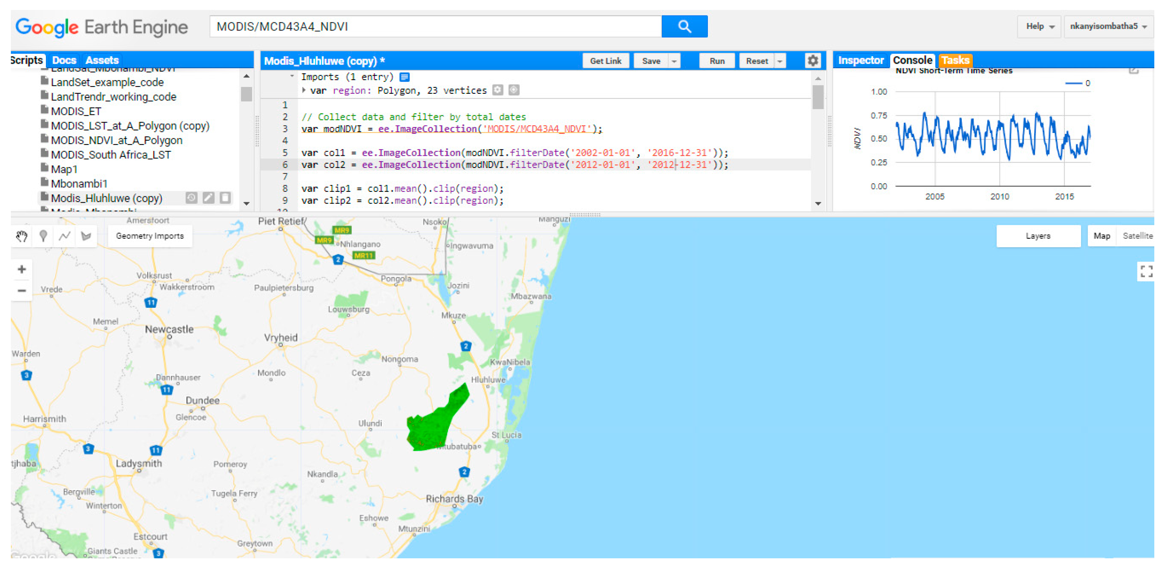
Here we show the Google Earth Engine interactive development environment. The dark green area indicates the location of the Hluhluwe-iMfolozi Park in north-eastern South Africa. The NDVI time series, which is averaged for the study area, is shown in the console part of the GEE interactive development environment.
Figure A1.
The Google Earth Engine interactive development environment.

References
- Stolton, S.; Dudley, N.; Avcıoğlu Çokçalışkan, B.; Hunter, D.; Ivanić, K.Z.; Kanga, E.; Kettunen, M.; Kumagai, Y.; Maxted, N.; Senior, J.; et al. Values and benefits of protected areas. In Protected Area Governance and Management; Worboys, G.L., Lockwood, M., Kothari, A., Feary, S., Pulsford, I., Eds.; ANU Press: Canberra, Australia, 2015; pp. 145–168. [Google Scholar]
- Kettunen, M.; ten Brink, P. Social and Economic Benefits of Protected Areas: An Assessment Guide; Routledge: Abingdon, UK, 2013. [Google Scholar]
- White, R.P.; Murray, S.; Rohweder, M.; Prince, S.D.; Thompson, K.M. Grassland Ecosystems; World Resources Institute: Washington, DC, USA, 2000. [Google Scholar]
- Sruthi, S.; Aslam, M.M. Agricultural drought analysis using the NDVI and land surface temperature data; a case study of Raichur district. Aquat. Procedia 2015, 4, 1258–1264. [Google Scholar] [CrossRef]
- Wilhite, D.A.; Svoboda, M.D.; Hayes, M.J. Understanding the complex impacts of drought: A key to enhancing drought mitigation and preparedness. Water Resour. Manag. 2007, 21, 763–774. [Google Scholar] [CrossRef] [Green Version]
- Myhre, G.; Shindell, D.; Bréon, F.M.; Collins, W.; Fuglestvedt, J.; Huang, J.; Koch, D.; Lamarque, J.F.; Lee, D.; Mendoza, B.; et al. Anthropogenic and Natural Radiative Forcing. In Climate Change 2013: The Physical Science Basis. Contribution of Working Group I to the Fifth Assessment Report of the Intergovernmental Panel on Climate Change; Tignor, K., Allen, M., Boschung, S.K., Nauels, J., Xia, Y., Bex, V., Midgley, P.M., Eds.; Cambridge University Press: Cambridge, UK; New York, NY, USA, 2013. [Google Scholar]
- Clark, P.U.; Shakun, J.D.; Marcott, S.A.; Mix, A.C.; Eby, M.; Kulp, S.; Levermann, A.; Milne, G.A.; Pfister, P.L.; Santer, B.D.; et al. Consequences of twenty-first-century policy for multi-millennial climate and sea-level change. Nat. Clim. Chang. 2016, 6, 360. [Google Scholar] [CrossRef]
- Duncan, J.M.; Biggs, E.M. Assessing the accuracy and applied use of satellite-derived precipitation estimates over Nepal. Appl. Geogr. 2012, 34, 626–638. [Google Scholar] [CrossRef]
- Dube, L.; Jury, M. The nature of climate variability and impacts of drought over KwaZulu-Natal, South Africa. S. Afr. Geogr. J. 2000, 82, 44–53. [Google Scholar] [CrossRef]
- Xulu, S.; Peerbhay, K.; Gebreslasie, M.; Ismail, R. Drought influence on forest plantations in Zululand, South Africa, using MODIS time series and climate data. Forests 2018, 9, 528. [Google Scholar] [CrossRef]
- Whateley, A. The Impact of Drought in the Hluhluwe Imfolozi Park (HiP) South Africa. 2017. Available online: http://theconservationimperative.com/?p=235 (accessed on 10 June 2018).
- Azzali, S.; Menenti, M. Mapping vegetation-soil-climate complexes in southern Africa using temporal Fourier analysis of NOAA-AVHRR NDVI data. Int. J. Remote Sens. 2000, 21, 973–996. [Google Scholar] [CrossRef]
- Hassan, M.H.; Hutchinson, C. Natural Resource and Environmental Information for Decision Making; The World Bank: Washington, DC, USA, 1992. [Google Scholar]
- Xie, Y.; Sha, Z.; Yu, M. Remote sensing imagery in vegetation mapping: A review. J. Plant Ecol. 2008, 1, 9–23. [Google Scholar] [CrossRef]
- Rulinda, C.M.; Dilo, A.; Bijker, W.; Stein, A. Characterizing and quantifying vegetative drought in East Africa using fuzzy modelling and NDVI data. J. Arid Environ. 2012, 78, 169–178. [Google Scholar] [CrossRef]
- Tucker, C.J. Red and photographic infrared linear combinations for monitoring vegetation. Remote Sens. Environ. 1979, 8, 127–150. [Google Scholar] [CrossRef] [Green Version]
- Poveda, G.; Salazar, L.F. Annual and interannual (ENSO) variability of spatial scaling properties of a vegetation index (NDVI) in Amazonia. Remote Sens. Environ. 2004, 93, 391–401. [Google Scholar] [CrossRef]
- Wang, J.; Rich, P.M.; Price, K.P.; Kettle, W.D. Relations between NDVI and tree productivity in the central Great Plains. Int. J. Remote Sens. 2004, 25, 3127–3138. [Google Scholar] [CrossRef] [Green Version]
- Sriwongsitanon, N.; Gao, H.; Savenije, H.H.G.; Maekan, E.; Saengsawan, S.; Thianpopirug, S. Comparing the Normalized Difference Infrared Index (NDII) with root zone storage in a lumped conceptual model. Hydrol. Earth Syst. Sci. 2016, 20, 3361–3377. [Google Scholar] [CrossRef]
- Sriwongsitanon, N.; Gao, H.; Savenije, H.H.G.; Maekan, E.; Saengsawan, S.; Thianpopirug, S. The Normalized Difference Infrared Index (NDII) as a proxy for soil moisture storage in hydrological modelling. Hydrol. Earth Syst. Sci. Discuss. 2015, 12, 8419–8457. [Google Scholar] [CrossRef]
- Joiner, J.; Yoshida, Y.; Anderson, M.; Holmes, T.; Hain, C.; Reichle, R.; Koster, R.; Middleton, E.; Zeng, F.W. Global relationships among traditional reflectance vegetation indices (NDVI and NDII), evapotranspiration (ET), and soil moisture variability on weekly timescales. Remote Sens. Environ. 2018, 219, 339–352. [Google Scholar] [CrossRef]
- Deshayes, M.; Guyon, D.; Jeanjean, H.; Stach, N.; Jolly, A.; Hagolle, O. The contribution of remote sensing to the assessment of drought effects in forest ecosystems. Ann. For. Sci. 2006, 63, 579–595. [Google Scholar] [CrossRef] [Green Version]
- Fensholt, R.; Rasmussen, K.; Nielsen, T.T.; Mbow, C. Evaluation of earth observation based long term vegetation trends—Intercomparing NDVI time series trend analysis consistency of Sahel from AVHRR GIMMS, Terra MODIS and SPOT VGT data. Remote Sens. Environ. 2009, 113, 1886–1898. [Google Scholar] [CrossRef]
- Hou, W.; Gao, J.; Wu, S.; Dai, E. Interannual variations in growing-season NDVI and its correlation with climate variables in the southwestern karst region of China. Remote Sens. 2015, 7, 11105–11124. [Google Scholar] [CrossRef]
- Xu, C.; Hantson, S.; Holmgren, M.; Nes, E.H.; Staal, A.; Scheffer, M. Remotely sensed canopy height reveals three pantropical ecosystem states. Ecology 2016, 97, 2518–2521. [Google Scholar] [CrossRef] [PubMed]
- Forkel, M.; Carvalhais, N.; Verbesselt, J.; Mahecha, M.D.; Neigh, C.S.; Reichstein, M. Trend change detection in NDVI time series: Effects of inter-annual variability and methodology. Remote Sens. 2013, 5, 2113–2144. [Google Scholar] [CrossRef]
- Liu, S.; Zhang, Y.; Cheng, F.; Hou, X.; Zhao, S. Response of grassland degradation to drought at different time-scales in Qinghai Province: Spatio-temporal characteristics, correlation, and implications. Remote Sens. 2017, 9, 1329. [Google Scholar]
- Jiang, L.; Shang, S.; Yang, Y.; Guan, H. Mapping interannual variability of maize cover in a large irrigation district using a vegetation index–phenological index classifier. Comput. Electron. Agric. 2016, 123, 351–361. [Google Scholar] [CrossRef]
- Cui, Y.P.; Liu, J.Y.; Hu, Y.F.; Kuang, W.H.; Xie, Z.L. An analysis of temporal evolution of NDVI in various vegetation-climate regions in Inner Mongolia, China. Procedia Environ. Sci. 2012, 13, 1989–1996. [Google Scholar] [CrossRef]
- Huang, F.; Mo, X.; Lin, Z.; Hu, S. Dynamics and responses of vegetation to climatic variations in Ziya-Daqing basins, China. Chin. Geogr. Sci. 2016, 26, 478–494. [Google Scholar] [CrossRef] [Green Version]
- Bond, W.J.; Archibald, S. Confronting complexity: Fire policy choices in South African savanna parks. Int. J. Wildl. Fire 2003, 12, 381–389. [Google Scholar] [CrossRef]
- Nsukwini, S.; Bob, U. The socio-economic impacts of ecotourism in rural areas: A case study of Nompondo and the Hluhluwe-iMfolozi Park (HiP). Afr. J. Hosp. Tour. Leis. 2016, 5, 1–15. [Google Scholar]
- Boundja, R.P.; Midgley, J.J. Patterns of elephant impact on woody plants in the Hluhluwe-imfolozi park, Kwazulu-Natal, South Africa. Afr. J. Ecol. 2010, 48, 206–214. [Google Scholar] [CrossRef]
- Trinkel, M.; Ferguson, N.; Reid, A.; Reid, C.; Somers, M.; Turelli, L.; Graf, J.; Szykman, M.; Cooper, D.; Haverman, P.; et al. Translocating lions into an inbred lion population in the Hluhluwe-iMfolozi Park, South Africa. Anim. Conserv. 2008, 11, 138–143. [Google Scholar] [CrossRef]
- Jolles, A.E.; Etienne, R.S.; Olff, H. Independent and competing disease risks: Implications for host populations in variable environments. Am. Nat. 2006, 167, 745–757. [Google Scholar] [CrossRef] [PubMed]
- Schaaf, C.B.; Gao, F.; Strahler, A.H.; Lucht, W.; Li, X.; Tsang, T.; Strugnell, N.C.; Zhang, X.; Jin, Y.; Muller, J.P. First operational BRDF, albedo nadir reflectance products from MODIS. Remote Sens. Environ. 2002, 83, 135–148. [Google Scholar] [CrossRef] [Green Version]
- Reinecker, M.M.; Suarez, M.J.; Gelaro, R.; Todling, R.; Bacmeister, J.; Liu, E.; Bosilovich, M.G.; Schubert, S.D.; Takacs, L.; Kim, G.K. MERRA: NASA’s modern-era retrospective analysis for research and applications. J. Clim. 2011, 24, 3624–3648. [Google Scholar] [CrossRef]
- Rodell, M.; Houser, P.R.; Jambor, U.E.A.; Gottschalck, J.; Mitchell, K.; Meng, C.J.; Arsenault, K.; Cosgrove, B.; Radakovich, J.; Bosilovich, M.; et al. The global land data assimilation system. Bull. Am. Meteorol. Soc. 2004, 85, 381–394. [Google Scholar] [CrossRef]
- Kruger, A. The influence of the decadal-scale variability of summer rainfall on the impact of El Niño and La Niña events in South Africa. Int. J. Climatol. 1999, 19, 59–68. [Google Scholar] [CrossRef] [Green Version]
- Anyamba, A.; Tucker, C.J.; Mahoney, R. From El Niño to La Niña: Vegetation response patterns over east and southern Africa during the 1997–2000 period. J. Clim. 2002, 15, 3096–3103. [Google Scholar] [CrossRef]
- Saji, N.H.; Goswami, B.N.; Vinayachandran, P.N.; Yamagata, T. A dipole mode in the tropical Indian Ocean. Nature 1999, 401, 360. [Google Scholar] [CrossRef] [PubMed]
- Reason, C.; Mulenga, H. Relationships between South African rainfall and SST anomalies in the southwest Indian Ocean. Int. J. Climatol. 1999, 19, 1651–1673. [Google Scholar] [CrossRef]
- Reason, C. Subtropical Indian Ocean SST dipole events and southern African rainfall. Geophys. Res. Lett. 2001, 28, 2225–2227. [Google Scholar] [CrossRef] [Green Version]
- Reason, C.; Rouault, M. ENSO-like decadal variability and South African rainfall. Geophys. Res. Lett. 2002, 29, 161–164. [Google Scholar] [CrossRef]
- Mann, H.B. Nonparametric tests against trend. Econometrica 1945, 1, 245–259. [Google Scholar] [CrossRef]
- Gilbert, R.O. Statistical Methods for Environmental Pollution Monitoring; John Wiley & Sons: Toronto, ON, Canada, 1987. [Google Scholar]
- Kendall, M.G. Rank Correlation Methods; Griffin: London, UK, 1975. [Google Scholar]
- Lanzante, J.R. Resistant, robust and non-parametric techniques for the analysis of climate data: Theory and examples, including applications to historical radiosonde station data. Int. J. Climatol. 1996, 16, 1197–1226. [Google Scholar] [CrossRef]
- Pohlert, T. Non-Parametric Trend Tests and Change-Point Detection. 2018. Available online: https://cran.r-project.org/web/packages/trend/trend.pdf (accessed on 27 July 2018).
- Sneyers, R. On the Statistical Analysis of Series of Observations; Technical Note No. 143, WMO No. 415; World Meteorological Organization: Geneva, Switzerland, 1991; p. 192. [Google Scholar]
- Mosmann, V.; Castro, A.; Fraile, R.; Dessens, J.; Sanchez, J.L. Detection of statistically significant trends in the summer precipitation of mainland Spain. Atmos. Res. 2004, 70, 43–53. [Google Scholar] [CrossRef]
- Chatterjee, S.; Bisai, D.; Khan, A. Detection of approximate potential trend turning points in temperature time series (1941–2010) for Asansol Weather Observation Station, West Bengal, India. India Atmos. Clim. Sci. 2014, 4, 64–69. [Google Scholar] [CrossRef]
- Zarenistanak, M.; Dhorde, A.G.; Kripalani, R.H. Trend analysis and change point detection of annual and seasonal precipitation and temperature series over southwest Iran. J. Earth Syst. Sci. 2014, 123, 281–295. [Google Scholar] [CrossRef]
- Soltani, M.; Rousta, I.; Taheri, S.S.M. Using Mann-Kendall and time series techniques for statistical analysis of long-term precipitation in Gorgan weather station. World Appl. Sci. J. 2013, 28, 902–908. [Google Scholar]
- Torrence, C.; Compo, G.P. A practical guide to wavelet analysis. Bull. Am. Meteorol. Soc. 1998, 79, 61–78. [Google Scholar] [CrossRef]
- Jevrejeva, S.; Moore, J.; Grinsted, A. Influence of the arctic oscillation and El Niño-Southern Oscillation (ENSO) on ice conditions in the Baltic Sea: The wavelet approach. J. Geophys. Res. Atmos. 2003, 108, 4677. [Google Scholar] [CrossRef]
- Grinsted, A.; Moore, J.C.; Jevrejeva, S. Application of the cross wavelet transform and wavelet coherence to geophysical time series. Nonlinear Proc. Geophys. 2004, 11, 561–566. [Google Scholar] [CrossRef] [Green Version]
- Zar, J.H. Biostatistical Analysis; Prentice Hall: Upper Saddle River, NJ, USA, 1999. [Google Scholar]
- Schulte, J.A.; Najjar, R.G.; Li, M. The influence of climate modes on streamflow in the Mid-Atlantic region of the United States. J. Hydrol. Reg. Stud. 2016, 5, 80–99. [Google Scholar] [CrossRef]
- Mberego, S.; Gwenzi, J. Temporal patterns of precipitation and vegetation variability over Zimbabwe during extreme dry and wet rainfall seasons. J. Appl. Meteorol. Climatol. 2014, 53, 2790–2804. [Google Scholar] [CrossRef]
- Manatsa, D.; Mukwada, G.; Siziba, E.; Chinyanganya, T. Analysis of multidimensional aspects of agricultural droughts in Zimbabwe using the standardized precipitation index (SPI). Theor. Appl. Climatol. 2010, 102, 287–305. [Google Scholar] [CrossRef]
- Verbesselt, J.; Hyndman, R.; Newnham, G.; Culvenor, D. Detecting trend and seasonal changes in satellite image time series. Remote Sens. Environ. 2010, 114, 106–115. [Google Scholar] [CrossRef]
- Verbesselt, J.; Hyndman, R.; Zeileis, A.; Culvenor, D. Phenological change detection while accounting for abrupt and gradual trends in satellite image time series. Remote Sens. Environ. 2010, 114, 2970–2980. [Google Scholar] [CrossRef] [Green Version]
- Fitchett, J.M.; Grab, S.W. A 66-year tropical cyclone record for south-east Africa: Temporal trends in a global context. Int. J. Climatol. 2014, 34, 3604–3615. [Google Scholar] [CrossRef]
- Islam, M.M.; Mamun, M.M.I. Variations of NDVI and its association with rainfall and evapotranspiration over Bangladesh. Rajshahi Univ. J. Sci. Eng. 2015, 43, 21–28. [Google Scholar] [CrossRef]
- Tabari, H.; Marofi, S.; Aeini, A.; Talaee, P.H.; Mohammadi, K. Trend analysis of reference evapotranspiration in the western half of Iran. Agric. For. Meteorol. 2011, 151, 128–136. [Google Scholar] [CrossRef]
- Crous, C.J.; Greyling, I.; Wingfield, M.J. Dissimilar stem and leaf hydraulic traits suggest varying drought tolerance among co-occurring Eucalyptus grandis × E. urophylla clones. South. For. J. For. Sci. 2018, 80, 175–184. [Google Scholar] [CrossRef]
Figure 1.
The study area showing the Hluhluwe-iMfolozi Park in the north-eastern part of South Africa.
Figure 1.
The study area showing the Hluhluwe-iMfolozi Park in the north-eastern part of South Africa.

Figure 2.
The standardized monthly Niño3.4 (a) and dipole mode index (DMI) (b) time series for the period from 1980 to 2017.
Figure 2.
The standardized monthly Niño3.4 (a) and dipole mode index (DMI) (b) time series for the period from 1980 to 2017.

Figure 3.
The spatiotemporal variability of normalized difference vegetation index (NDVI) at the Hluhluwe-iMfolozi Park for the period from 2002 to 2017. The scale represents the range of NDVI values from 0 to 1.
Figure 3.
The spatiotemporal variability of normalized difference vegetation index (NDVI) at the Hluhluwe-iMfolozi Park for the period from 2002 to 2017. The scale represents the range of NDVI values from 0 to 1.

Figure 4.
(a) The deseasonalized monthly mean NDVI time series for HiP. The continuous red line indicates the trend estimate and the dashed red lines show the 95% confidence interval for the trend based on resampling methods. (b,c) show the histogram and yearly mean time series, respectively.
Figure 4.
(a) The deseasonalized monthly mean NDVI time series for HiP. The continuous red line indicates the trend estimate and the dashed red lines show the 95% confidence interval for the trend based on resampling methods. (b,c) show the histogram and yearly mean time series, respectively.

Figure 5.
The monthly mean time series values of (a) NDVI, (b) Enhanced Vegetation Index (EVI), (c) Burned Area (BAI), and Modern Retrospective Analysis for the Research Application (MERRA-2) model soil temperature (d) and precipitation (e), Global Land Data Assimilation System (GILDAS) evapotranspiration (f) and Normalized Difference Infrared Index (NDII) (g). The dotted lines represent the 12-month smooth trends.

Figure 6.
The (a,b) NDVI, (c,d) EVI and (e,f) BAI (blue dashed line) 12-month smooth trends versus Niño3.4 (left panels) and DMI (right panels) for the period from 2002 to 2017 for the HiP.
Figure 6.
The (a,b) NDVI, (c,d) EVI and (e,f) BAI (blue dashed line) 12-month smooth trends versus Niño3.4 (left panels) and DMI (right panels) for the period from 2002 to 2017 for the HiP.

Figure 7.
The heat map of Pearson correlation coefficients for NDVI, NDII, precipitation (Prec), soil temperature (Soil.Temo), ET, BAI, Niño3.4, and DMI.
Figure 7.
The heat map of Pearson correlation coefficients for NDVI, NDII, precipitation (Prec), soil temperature (Soil.Temo), ET, BAI, Niño3.4, and DMI.

Figure 8.
The inter-annual variability of linear correlations between NDVI and BAI, Soil Temp, Prec, Niño3.4, DMI, ET, and NDII for the period 2002 to 2017.
Figure 8.
The inter-annual variability of linear correlations between NDVI and BAI, Soil Temp, Prec, Niño3.4, DMI, ET, and NDII for the period 2002 to 2017.

Figure 9.
(a) The inter-annual variation of Mann–Kendall z-scores (α = 0.05, Z1 = –1.96, Z2 = 1.96) for the HiP from 2002 to 2017. (b) Sequential statistics values of progressive (Prog) (solid red line) and retrograde (black solid line) obtained by Sequential Mann-Kendall (SQ-MK) test for HiP monthly mean NDVI data for the period from 2002 to 2017.

Figure 10.
The normalized wavelet power spectra of monthly mean (a) NDVI, (b) precipitation, (c) Soil temperature, (d) DMI, (e) Niño3, (f) NDII, and (g) ET, plotted for the period from 2002 to 2017. The black lines which encircle the yellowish colors indicate the areas of significance at the 95% confidence level using the red noise model.

Figure 11.
The squared cross-wavelet power spectra for NDVI–Niño3.4, NDVI–DMI, NDVI-precipitation, NDVI–soil temperature, NDVI–NDII, and NDVI–ET. The continuous black lines demarcate the areas of significance at the 95% confidence level using the red noise model. The arrows are vectors indicating the phase difference between the cross-wavelet parameters (see the legend in the bottom left corner).


Table 1.
The output of the Multiple Linear Regression (MLR) model in which Normalized Difference Vegetation Index (NDVI) is a dependent variable and soil temperature, precipitation (Soil Temp), Niño3.4, Normalized Difference Infrared Index (NDII), Dipole Model Index (DMI), and Evapotranspiration (ET) are independent variables.
| Variable | Estimate | Std. Error | t-Value | p-Value | Sig |
|---|---|---|---|---|---|
| Soil. Temp | −1.23 × 10−02 | 3.39 × 10−03 | −3.615 | 0.000386 | *** |
| Prec | 7.35 × 10−05 | 1.72 × 10−04 | 0.427 | 0.669736 | |
| Niño3.4 | −6.44 × 10−03 | 7.62 × 10−03 | −0.845 | 0.399427 | |
| NDII | 1.46 × 10+00 | 7.60 × 10−02 | 19.214 | <2.00 × 10⁻¹⁶ | *** |
| ET | 4.03 × 10+03 | 1.05 × 10+03 | 3.833 | 0.000173 | *** |
Significance codes: 0 ‘***’ 0.001 ‘**’ 0.01 ‘*’ 0.05 ‘.’ 0.1 ‘ ’ 1.
© 2018 by the authors. Licensee MDPI, Basel, Switzerland. This article is an open access article distributed under the terms and conditions of the Creative Commons Attribution (CC BY) license (http://creativecommons.org/licenses/by/4.0/).
Share and Cite
MDPI and ACS Style
Mbatha, N.; Xulu, S. Time Series Analysis of MODIS-Derived NDVI for the Hluhluwe-Imfolozi Park, South Africa: Impact of Recent Intense Drought. Climate 2018, 6, 95. https://0-doi-org.brum.beds.ac.uk/10.3390/cli6040095
AMA Style
Mbatha N, Xulu S. Time Series Analysis of MODIS-Derived NDVI for the Hluhluwe-Imfolozi Park, South Africa: Impact of Recent Intense Drought. Climate. 2018; 6(4):95. https://0-doi-org.brum.beds.ac.uk/10.3390/cli6040095
Chicago/Turabian StyleMbatha, Nkanyiso, and Sifiso Xulu. 2018. "Time Series Analysis of MODIS-Derived NDVI for the Hluhluwe-Imfolozi Park, South Africa: Impact of Recent Intense Drought" Climate 6, no. 4: 95. https://0-doi-org.brum.beds.ac.uk/10.3390/cli6040095
Note that from the first issue of 2016, this journal uses article numbers instead of page numbers. See further details here.