The 10-Year Return Levels of Maximum Wind Speeds under Frozen and Unfrozen Soil Forest Conditions in Finland


1
Weather and Climate Change Impact Research, Meteorological and Marine Research Programme, Finnish Meteorological Institute, P.O. Box 503, FI-00101 Helsinki, Finland
2
School of Forest Sciences, Faculty of Science and Forestry, University of Eastern Finland, Yliopistonkatu 7, FI-80101 Joensuu, Finland
*
Author to whom correspondence should be addressed.
Climate 2019, 7(5), 62; https://0-doi-org.brum.beds.ac.uk/10.3390/cli7050062
Submission received: 8 March 2019
/
Revised: 25 April 2019
/
Accepted: 29 April 2019
/
Published: 30 April 2019
(This article belongs to the Special Issue Climate Variability and Change in the 21th Century)
Abstract
:Reliable high spatial resolution information on the variation of extreme wind speeds under frozen and unfrozen soil conditions can enhance wind damage risk management in forestry. In this study, we aimed to produce spatially detailed estimates for the 10-year return level of maximum wind speeds for frozen (>20 cm frost depth) and unfrozen soil conditions for dense Norway spruce stands on clay or silt soil, Scots pine stands on sandy soil and Scots pine stands on drained peatland throughout Finland. For this purpose, the coarse resolution estimates of the 10-year return levels of maximum wind speeds based on 1979–2014 ERA-Interim reanalysis were downscaled to 20 m grid by using the wind multiplier approach, taking into account the effect of topography and surface roughness. The soil frost depth was estimated using a soil frost model. Results showed that due to a large variability in the timing of annual maximum wind speed, differences in the 10-year return levels of maximum wind speeds between the frozen and unfrozen soil seasons are generally rather small. Larger differences in this study are mostly found in peatlands, where soil frost seasons are notably shorter than in mineral soils. Also, the high resolution of wind multiplier downscaling and consideration of wind direction revealed some larger local scale differences around topographic features like hills and ridgelines.
1. Introduction
In the last few decades, wind storms have caused the most damage and economic losses in European forests, compared to all abiotic and biotic damage agents [1,2,3,4]. So far, winter storms have caused the most destructive damage in Western and Central Europe [3,5,6], e.g., storms like Vivian in 1990 (over 100 million m3 of timber), Lothar and Martin in 1999 (over 175 million m3), Kyrill in 2007 (54 million m3) and Klaus in 2009 (50 million m3), respectively. Damages have increased in recent years also in northern Europe [4,6,7], where in 2015 Gudrun damaged 70 million m3 and in 2007 Per damaged 12 million m3 of timber, mainly in Sweden. In Finland, over 25 million m3 of timber has been damaged during storms since 2000, the most in autumn storms in 2001 (Pyry and Janika, 7.3 million m3) and in summer storm in 2010 (Asta, Veera, Lahja and Sylvi, 8 million m3), respectively. The increasing amount of damages in European forests may at least partially be explained by increasing volume of growing stock and changes in forest structure (e.g., age, tree species) related to changes in forest management practices [1,5,8,9]. Forest disturbances may also amplify or even cancel out the expected increase in productivity of forests under changing climate [4,10].
Some recent studies indicate increased storminess for some regions in Europe (see e.g., review by [11]). However, the majority of studies point towards decadal variation in storminess without any clear trend for a direction or another [12,13,14,15]. In Finland, slight weakening of annual mean (−0.09 ms−1 decade−1) and maximum (−0.32 ms−1 decade−1) wind speeds across 33 weather stations have been observed in the period of 1959–2015 [16], which is in accordance with widespread weakening of terrestrial near-surface wind speeds [17,18]. For future projections, the change in the extreme wind speed during the coming decades is still a somewhat unsolved issue and the outcome is largely dependent on the climate model used for the simulation [11,19,20].
However, the risk of wind damage to forests may still increase in Northern Europe under climate change even if the frequency and severity of wind storms do not increase. This is due to the shortening of the frozen soil period, which improves tree anchorage during the windiest season of the year from late autumn to early spring [21,22,23,24]. Moreover, storms may be accompanied by heavier rainfall, leading to more saturated soils and increased risk of wind damage [5]. When estimating the forest wind damage risk it is thus essential to know whether the extreme wind speeds occur during the frozen or unfrozen soil conditions. Typically, the windiest season in Finland is from October to March [25] and soil frost season starts in October–November and ends in April–May [26]. However, there is large year-to-year and regional variation in soil frost duration.
Even a 20 cm thick frozen soil increases the anchorage of trees and reduces substantially the risk of uprooting [27,28]. According to tree-pulling experiments in Finland, under frozen soil the type of failure was stem breakage, whereas under unfrozen soil conditions, about 80% of trees uprooted, respectively [28]. From the three economically and ecologically most important boreal tree species in Finland, Norway spruce (Picea abies) with the shallow rooting is the most vulnerable to uprooting, followed by Silver and Downy birches (Betula pendula and Betula pubescens), and Scots pine (Pinus sylvestris), respectively [27,28]. However, from late autumn to early spring, birches (without leaves) are not vulnerable to wind damage and therefore excluded from this study.
For snow free surfaces, the soil frost modelling can be done using cold season frost sum and soil characteristics alone [29]. The presence of snow and vegetation complicates the modelling, and requires a more sophisticated approach including the modelling of heat and water transfer [23]. An example of a relatively simple approach accounting for the main controlling factors was published by [30]. It was further developed and tested in the Finnish conditions by [31] for the calculation of soil temperatures in three common combinations of soil and forest types in Finland, i.e., dense Norway spruce stands on clay or silt soil, Scots pine stands on sandy soil, and Scots pine stands on drained peatlands. Soil frost conditions can vary a lot, even up to few months in mean duration, depending on soil type. Peat is effective insulator compared to mineral soils, therefore having shorter soil frost periods in similar climatic conditions [31].
The estimation of the return levels of maximum wind speed values (extreme winds) can be done using observational data representing conditions at the observing station location or using reanalyzed data like ERA-Interim [32], representing a larger area’s averaged value, respectively. When studying the high-resolution spatial variation of extreme winds, the data has to be either downscaled from the reanalyzed coarse grid to a local value or upscaled from station point observations to areas located between the stations. Downscaling can be done by applying various spatial statistical tools, e.g., [33,34], or complex airflow models like e.g., WAsP [35], which are typically applied for wind power potential predictions. GIS-based methods for mapping the areas having highest wind damage risk have also been introduced, e.g., [36,37,38]. One computationally feasible approach for the estimation of the return levels of extreme wind speeds for large geographical areas with very high spatial resolution is the wind multiplier approach [39,40,41]. In this method, return levels obtained, e.g., from the reanalysed data, are downscaled to local wind speeds with help of land cover (roughness) and topography data. By applying GIS-tools such as ArcGIS, QGIS or R, it is rather straightforward to produce the required multipliers.
The reliable high-resolution information on the spatial variation of extreme wind speeds can enhance wind damage risk management in forest planning and forestry. In the above context, the objective of this study was to produce spatially detailed estimates (maps) of the 10-year return level maximum wind speed under current climate for unfrozen and frozen soil conditions in some of the most common combinations of forest and soil types in Finland. By utilizing soil frost calculations of [31] to determine the duration of soil frost seasons, the wind speed return level calculations were done for dense Norway spruce stands on clay or silt soil, Scots pine stands on sandy soil, and Scots pine stands on drained peatland. The coarse resolution estimates of the 10-year return level of maximum wind speed were based on 1979–2014 ERA-Interim dataset [32]. Downscaling to a 20 m grid was done by applying the wind multiplier approach [41].
2. Materials and Methods
2.1. Soil Frost Modelling
Soil frost conditions were modelled by using an extended version of the original soil temperature model [30]. It was derived from the law of conservation of energy and mass assuming constant water content in the soil. Model was further developed to take into account the heat flow below soil layer of consideration [42]. Following [42], soil temperature at depth ZS (m) can be calculated as follows:
where (°C) is the soil temperature on a previous day, TAIR (°C) is the air temperature, Δt is the length of a time step (s), KT (W m−1 °C−1) is the thermal conductivity of the soil above ZS, CS (J m−3 °C−1) is the specific heat capacity of the soil above ZS, CICE (J m−3 °C−1) is the specific heat capacity due to freezing and thawing, fS (m−1) is an empirical damping parameter due to snow cover, DS (m) is snow depth, KT,LOW (W m−1 °C−1) is the thermal conductivity of the soil below ZS, CS,LOW (J m−3 °C−1) is specific heat capacity of the soil below ZS, and TLOW (°C) is soil temperature at the depth of Zl. Following to [31], Zl was set to 6.8 m.
By using soil temperature observations from several stations across Finland, the soil temperature model was parametrized for three different soil types: clay or silt soil, sandy soil, and peatlands [31]. Between the depths of 20 and 100 cm, the parametrized model explained approximately 90–99% of the observed variability in soil temperatures.
In a study by [31], also a snow depth model (based largely on the work of [43]) was used to simulate the snow depth, using daily temperature and precipitation observations [44], for different forest conditions in addition to open areas. In this study, we used the soil frost data calculated by [31] for different combinations of forest and soil types, based on combined use of soil temperature and snow depth model. The soil frost data in 0.1° × 0.2° grid has been calculated for dense spruce stands on clay or silt soil (hereafter CSS), pine stands on sandy soil (hereafter SP) and pine stands on peatlands (hereafter PP), respectively. Calculations for each of the forest and soil types were performed on every grid cell. The soil was assumed to be frozen and provide sufficient anchorage for trees when the modelled soil frost extended at least to a depth of 20 cm continuously from the surface and unfrozen otherwise. The expectation of the sufficient anchorage was based on the typical rooting depth of main boreal tree species, see e.g., [21,24,27,28].
2.2. Estimation of the 10-Year Return Levels of Wind Speed
The 10-year return levels, corresponding to an annual probability of exceeding the 90th percentile, of maximum wind speeds were calculated using the ERA-Interim dataset [32] covering years 1979–2014 and the generalized extreme value method (GEV) [45]. We used the block maxima approach, in this case for seasonal maximum wind speeds of both frozen and unfrozen soil season, with the maximum-likelihood fitting of GEV distribution [46,47]. We analysed 10-minute instantaneous wind speeds available at 6-hour intervals given as grid box averages, each covering an area of 0.75° × 0.75°.
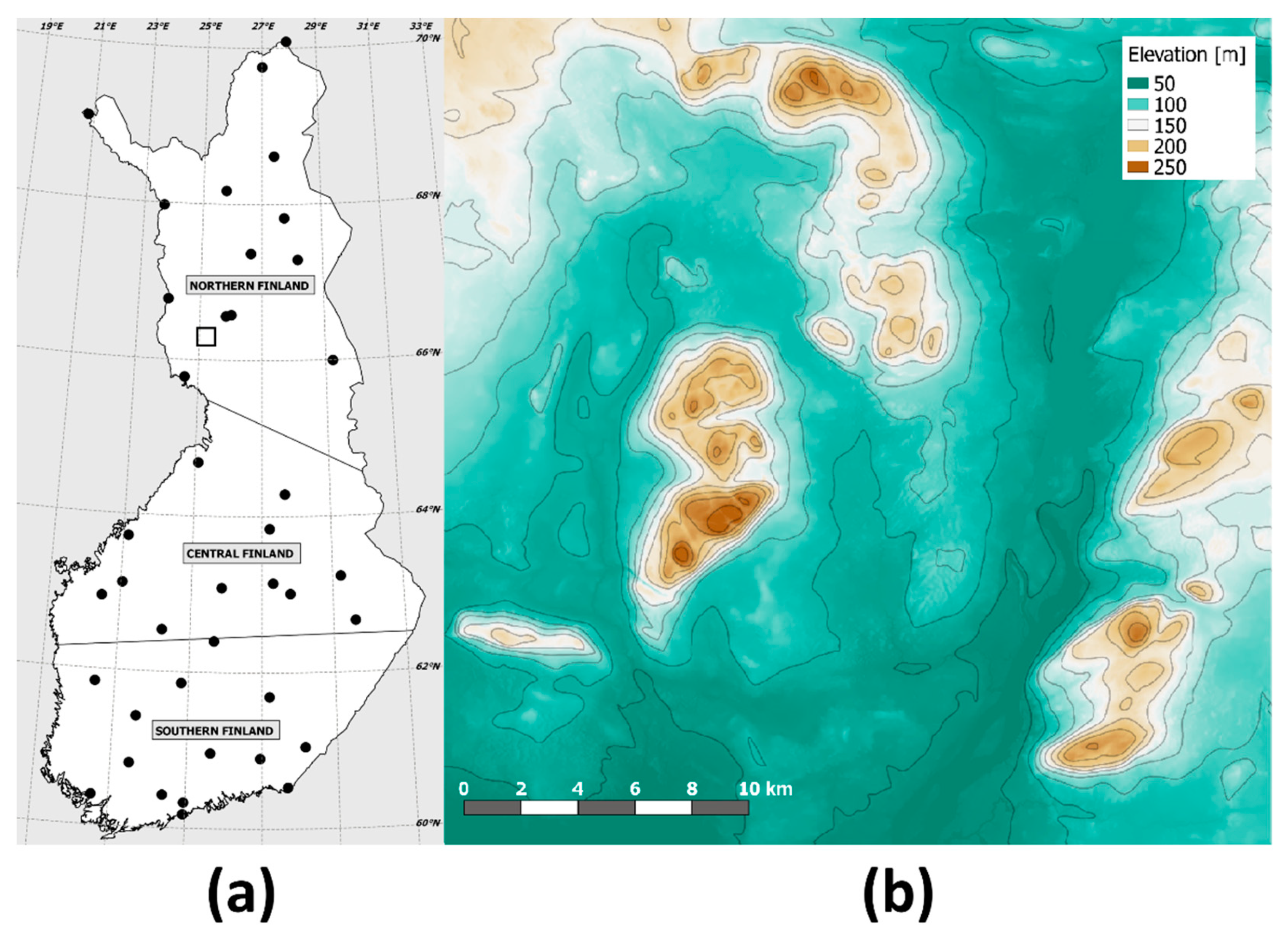
The maximum wind speed dependence on wind direction was estimated by making the calculations wind direction wise, i.e., the 10-year return levels were estimated separately for cardinal and intercardinal wind direction sectors. For comparison and validation purposes, 10-year return levels were also calculated for 40 weather stations (Figure 1a) across Finland (on mainland) using wind speed observations covering the same period of 1979–2014 as in the ERA-Interim dataset. Observational data consisted of synoptic observations of 10-minute average wind speed with 3-hour measurement interval.
Compared to our data period of 1979–2014, the 10-year return level estimates can be expected to be quite robust. Estimated 10-year return level, i.e., wind speed equalled or exceeded on average once every 10 years, is relatively short period compared to our data period of 35 years. However, in coastal regions of southern and southwestern Finland, uncertainties related to the statistical estimation of return level is somewhat increased. This applies particularly for PP as, based on soil frost calculations by [31], mild winters with no soil frost, or at least not exceeding 20 cm in depth, are quite common (not shown). In these cases, the dataset from which soil frost season return levels are calculated is smaller, leading to a wider return level estimate confidence intervals. Also, regions with only short soil frost period, when the window for seasons maximum wind speed can often be only e.g., 1–2 months, have larger variability in the used dataset for return level estimation, therefore increasing uncertainty even if totally frost-free years are rare.
Considering normal approximation 95% confidence intervals of calculated 10-year return level estimates for weather stations, range is on average +/−1 m/s over all 1920 return level calculations consisting of 40 stations, eight wind directions, three forest soil types, and distinction between frozen and unfrozen soil season, respectively.
2.3. Downscaling of the 10-Year Return Levels of Wind Speed
The impact of local terrain features on maximum wind speed cannot fully be taken into account in the relatively coarse 0.75° × 0.75° grid of ERA-Interim, because for example, hills, lakes, and changes in land-use are not considered in detail. For this reason, in order to downscale the wind speed return level from the coarse grid to a high-resolution grid we used a wind multiplier approach tested recently by [41] for boreal forest conditions. In this study, only topographic and terrain (surface roughness) properties are taken into account when assessing local maximum wind speeds (and their return levels) separately for the eight cardinal and intercardinal wind directions. For the application in forested landscapes, the shielding factor, i.e., the effect of upwind buildings providing cover to the place of interest and only relevant in urban areas, was not considered. The wind multiplier method has been presented earlier in [40,48] for more details.
Following the study by [41], the return level of regional maximum wind speed (UR) in an open terrain at a 10-m height is downscaled into site-specific return level (Usite) by applying two multipliers, i.e., terrain multiplier (Mz), and topographic (hill-shape) multiplier (Mh):
We used a 20 × 20-m grid, which is in line with the CORINE Land Cover 2012 dataset [49] providing the information on land cover and land use that enabled the calculation of terrain multiplier. When defining the terrain multiplier (Mz), we used a 500 m fetch length and weighted the grid points close to place of interest more than the further upwind grid points.
The topographic (hill-shape) multiplier (Mh) was calculated by taking into account the variations and change of elevation 1000 m upwind from the place of interest. As well, the elevation of the place of interest was taken into account. Development of the Mz and Mh multipliers used in this study were described more elaborately in the Sections 2.3 and 2.4 of [41]. According to [41], for areas with no extreme variations of elevation, the wind multiplier approach was a feasible method to identify at a high spatial resolution locations having the highest forest wind damage risks.
2.4. Comparison of Return Levels Derived from Point Observations, Reanalysed Data, and Wind Multiplier Downscaled Data
The 10-year return levels of maximum wind speeds calculated from the observations (OBS) of 40 weather stations (Figure 1a) were compared to corresponding return levels calculated from the original ERA-Interim reanalysed data (ERA) and return levels downscaled with wind multiplier approach (WM). Weather station location coordinates were used to derive data from ERA and WM gridded datasets.
Besides general visual scatterplot comparison of ERA and WM values to OBS values, also the coefficient of determination R2, D statistic of two-sample Kolmogorov–Smirnov test, and mean differences were used to analyse the performance of ERA and WM to produce return level values similar to OBS. These statistics were also analysed at the station level. Comparisons were considered more at a qualitative than quantitative level, i.e., are return level values produced with WM approach improvement to original ERA values when considering similarity to values derived from weather station observations.
The D statistic of the two-sample Kolmogorov–Smirnov test was used as a measure of similarity of ERA and WM to OBS. Smaller values of D are considered as a good result, i.e., EDF (empirical distribution function) of WM is more similar than EDF of ERA compared to EDF of OBS. Mean difference statistic used was simply the mean of differences between ERA and WM to OBS at station level, over all the combinations of eight wind directions, three soil types, and distinction between frozen and unfrozen soil. Again, smaller values were considered as a good result as a difference between WM and OBS is smaller than a difference between ERA and OBS. R2 was used as a goodness of fit of a simple linear regression between OBS and ERA or WM. Here, increasing R2 was considered as an improvement when comparing a regression of OBS and WM to a regression of OBS and ERA.
2.5. Structure and Restrictions of Data Analyses
For deeper understanding of results for calculated return levels of maximum wind speeds and their differences between frozen and unfrozen soil, we first considered independently underlying soil frost conditions (e.g., number of soil frost days and duration of soil frost) and wind conditions (e.g., timing of maximum wind speeds throughout year and between frozen and unfrozen seasons), respectively.
We also restricted our analysis to mainland Finland (see Figure 1a). The reasoning for this is the lack of years with soil frost in the archipelago, leading to increased uncertainty in the calculation of wind speed return levels. Also, the insufficient performance of wind multiplier method for the small Baltic Sea islands found by [41] supports our decision.
The territory of Finland was moreover divided into three sub-regions in the analysis of results. The three sub-regions were based roughly on the mean annual growing degree day sum (GDD) calculated using the threshold of 5 °C. The limits are GDD > 1200 °C days for southern, 1000 °C days < GDD ≤ 1200 °C days for central and GDD ≤ 1000 °C days for northern sub-regions, following also roughly the borders of boreal subzones.
Also, one smaller area (30 × 30 km) from northern Finland (Figure 1a) with a more complex topography (Figure 1b) was used to examine and present the more local scale behavior and influences of wind multiplier downscaling to 10-year return levels of wind speeds and differences between frozen and unfrozen soil seasons.
3. Results
3.1. Soil Frost Conditions
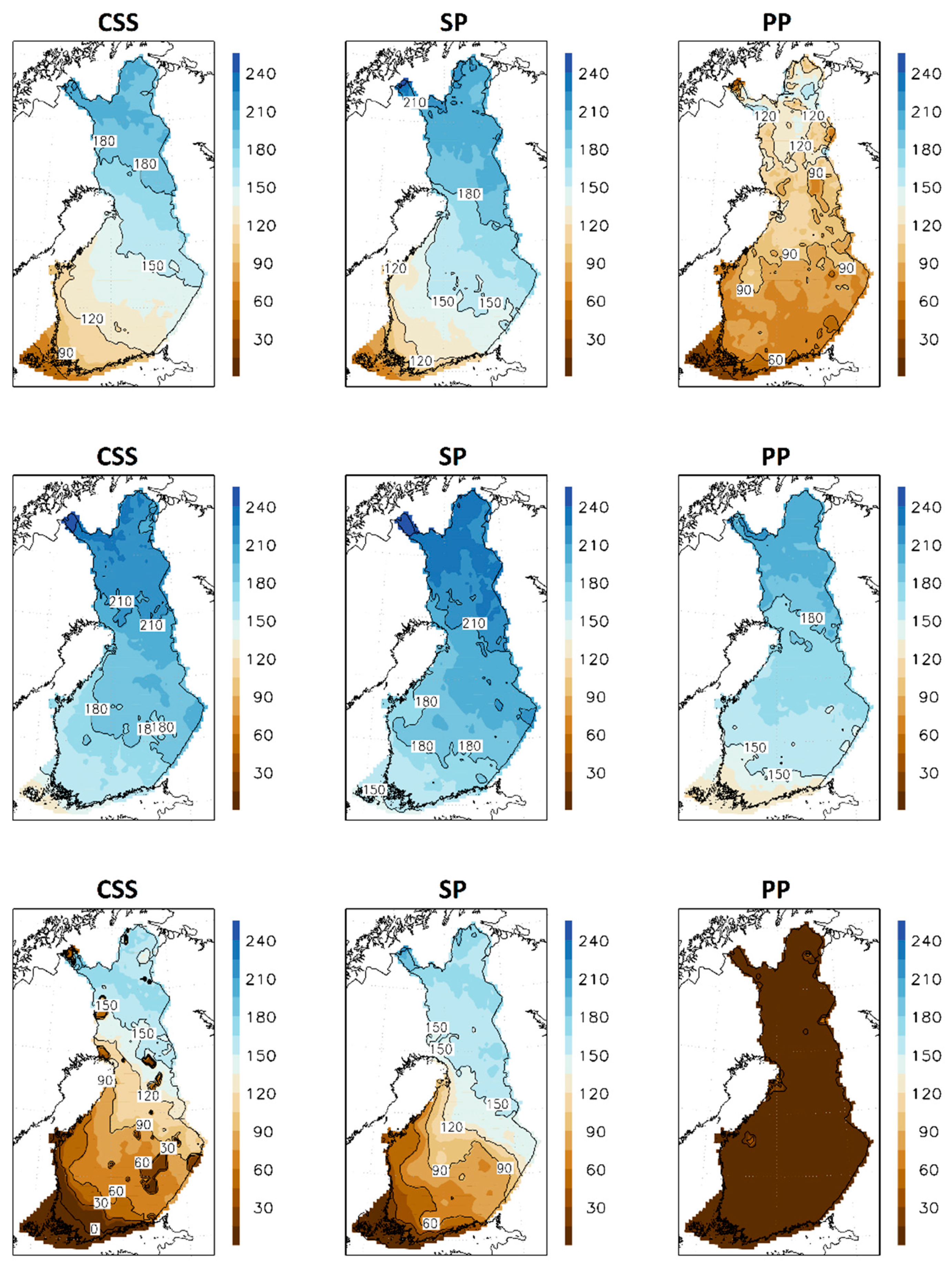
Figure 2 presents the modelled annual mean, minimum and maximum number of soil frost days for three different forest and soil-type combinations in the period 1979–2014. In general, upland forests on sandy soil had the most soil frost days and forests on drained peatlands least. Duration of soil frost season in northern Finland was on average approximately 5–7 months for dense spruce stands on clay or silt soil (CSS) and pine stands on sandy soil (SP). For pine stands on peatlands (PP) soil frost season was considerably shorter, 3–5 months, with large spatial variability. In the central parts of the country, the season lasts on average about 3–4 months for PP and roughly 4–6 months for SP and CSS. Length of the average soil frost season in southern Finland range from less than two months in the coastal areas for PP up to five months for SP in the northern part of southern Finland.
However, especially for PP, frost-free seasons are possible almost everywhere in Finland. For SP, soil frost season can also be as short as about a month in southern and southwestern coastal areas. Conversely for SP, soil frost season is at least 5 months long in the whole northern part of Finland. The maximum length of soil frost season differs less from the average than the minimum. Here CSS and SP are quite similar, the maximum length of frost season ranging from about 5 months even at the coast to over 8 months in the most northwestern part of Finland. For PP, the longest soil frost periods are roughly a month shorter.
Years with zero soil frost days are virtually nonexistent in CSS and SP, but in PP there are rather large areas with roughly one-third of the 36-year study period with no soil frost (not shown). These areas are mainly in the southern part of Finland, but also in the northern parts, respectively. Years with less than 60 soil frost days are rare in CSS and SP apart from the southwestern part of Finland, where especially in coastal areas about every third year is this kind. Again, PP is substantially different with some areas having a majority of years with soil frost season less than 60 days.
3.2. Wind Conditions
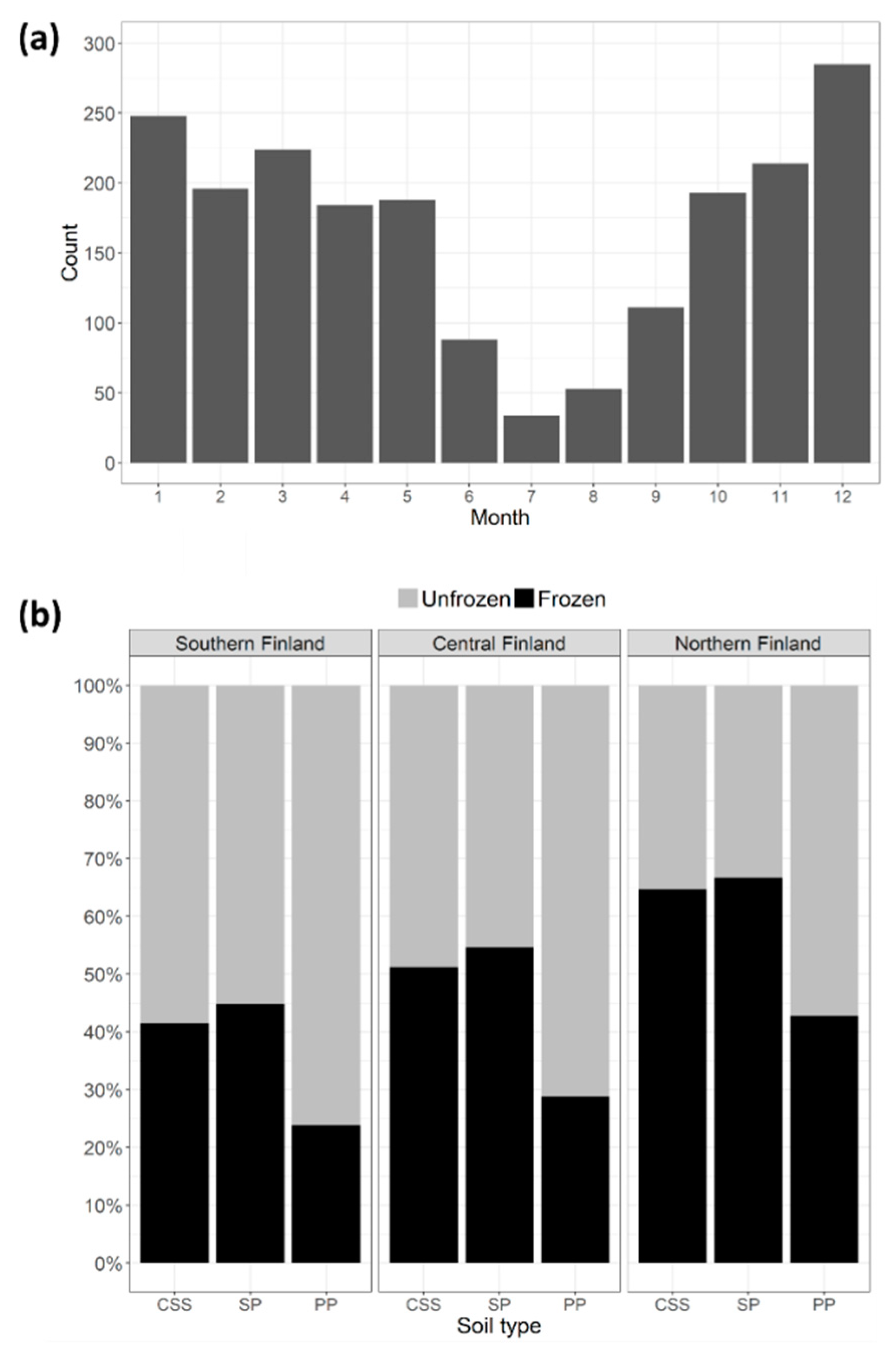
We found large year-to-year variability in the timing of the annual maximum wind speed in the period 1979–2014. Among all 40 stations, the most common month for annual maximum wind speed was December (Figure 3a). However, also months from October to May are rather common for annual maximum wind speeds. Direction wise the annual maximum wind speeds from N, NE, and E were most commonly observed during spring and early summer (April–June), whereas for rest of the directions it was usually observed from October to March (not shown).
It was rather common that the annual maximum wind speed was observed multiple times during a year, partly driven by wind observations having no digits in the first part of the study period. About 25% of all the years among 40 stations had annual maximum wind speeds observed on more than one month of that year. 49% for PP, 59% for CSS, and 62% for SP of these years were ones with similar maximums during frozen and unfrozen seasons (not shown).
Figure 3b presents how observed annual maximum wind speed was split up between frozen and unfrozen seasons on different forest and soil type combinations in southern (14 stations), central (12 stations), and northern (14 stations) Finland. The annual maximum wind speed was observed rather evenly in both seasons in the case of CSS and SP, occurring slightly more often during unfrozen season in southern Finland and frozen season in northern Finland, respectively. For PP the difference was more pronounced, especially in southern and central Finland where annual maximum wind speed was clearly more often observed during unfrozen season.
We also further compared the underlying distributions of seasonal maximum wind speeds, from where return level estimates for 40 stations were calculated, using two-sample Kolmogorov–Smirnov tests to determine if there was statistically significant (p < 0.05) difference between frozen and unfrozen soil seasons. For CSS, difference was statistically significant in southern and northern, and non-significant in central Finland. For SP, significant in central and northern, and non-significant in southern Finland. And for PP, significant in southern and central, and non-significant in northern Finland, respectively.
3.3. The 10-Year Return Levels of Maximum Wind Speed for Frozen vs. Unfrozen Soil
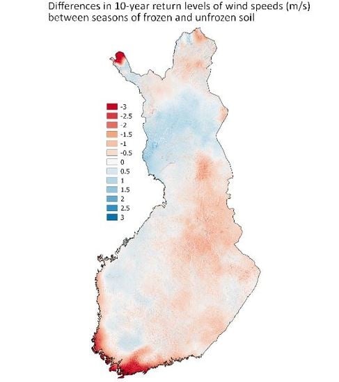
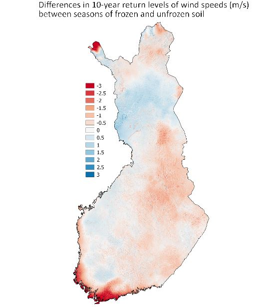
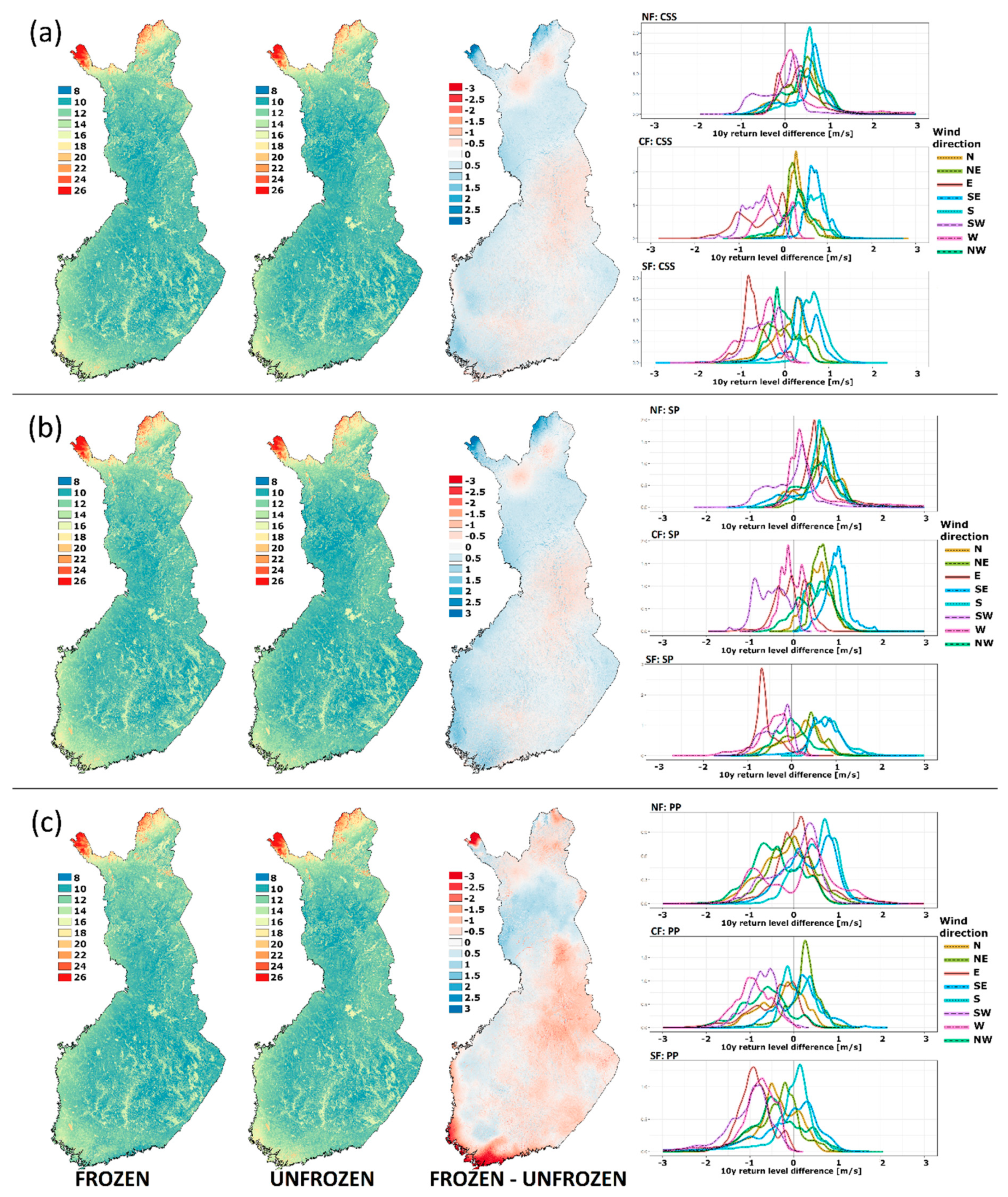
Generally differences in maximum 10-year return level of wind speed between seasons of frozen and unfrozen soil are rather small (difference +/−1 m/s) in large part of Finland. Small differences were observed especially for CSS (Figure 4a maps) and SP (Figure 4b maps), of which results as a whole resemble each other closely with similar spatial patterns and direction of differences. On large scale, larger differences were observed for CSS and SP only in parts of northernmost Finland and in the coastal are of southwestern Finland, i.e., maximum 10-year return level of wind speed was about 1–2 m/s larger in soil frost season. Differences larger than +/−1 m/s were a bit more common for PP (Figure 4c maps). Areas with stronger winds during the unfrozen season were found across coastal areas, parts of eastern Finland, and northernmost Finland, respectively. Noteworthy, compared to CSS and SP, sign of the difference is opposite in the coastal areas and in the most northwestern part of Finland. Notable positive differences in PP restricts to western and central parts of Lapland.
There were also some quite notable differences direction wise whether the bulk/peak of the distribution of differences was over or below zero (Figure 4a–c distributions). The effect of wind direction on distribution of differences was smallest in northern Finland, regardless of combination of forest and soil type. In southern Finland, for S and SE wind directions return level of wind speeds were stronger during soil frost season. Conversely, winds from W, SW, and E were characterized by stronger winds during unfrozen soil season, whereas for the rest of the directions, differences were more or less evenly distributed around zero. In central Finland, dependence on wind direction was similar for CSS and SP, with N, NE, SE, S, and NW directions having dominantly stronger winds during frozen soil season and W, SW, and E directions were characterized by stronger winds during unfrozen soil season or the differences were distributed rather evenly. For PP, more directions were characterized by stronger winds during unfrozen soil season, namely N, E, SW, W, and NW. Only NE, SE, and S directions had stronger winds mainly during frozen soil season.
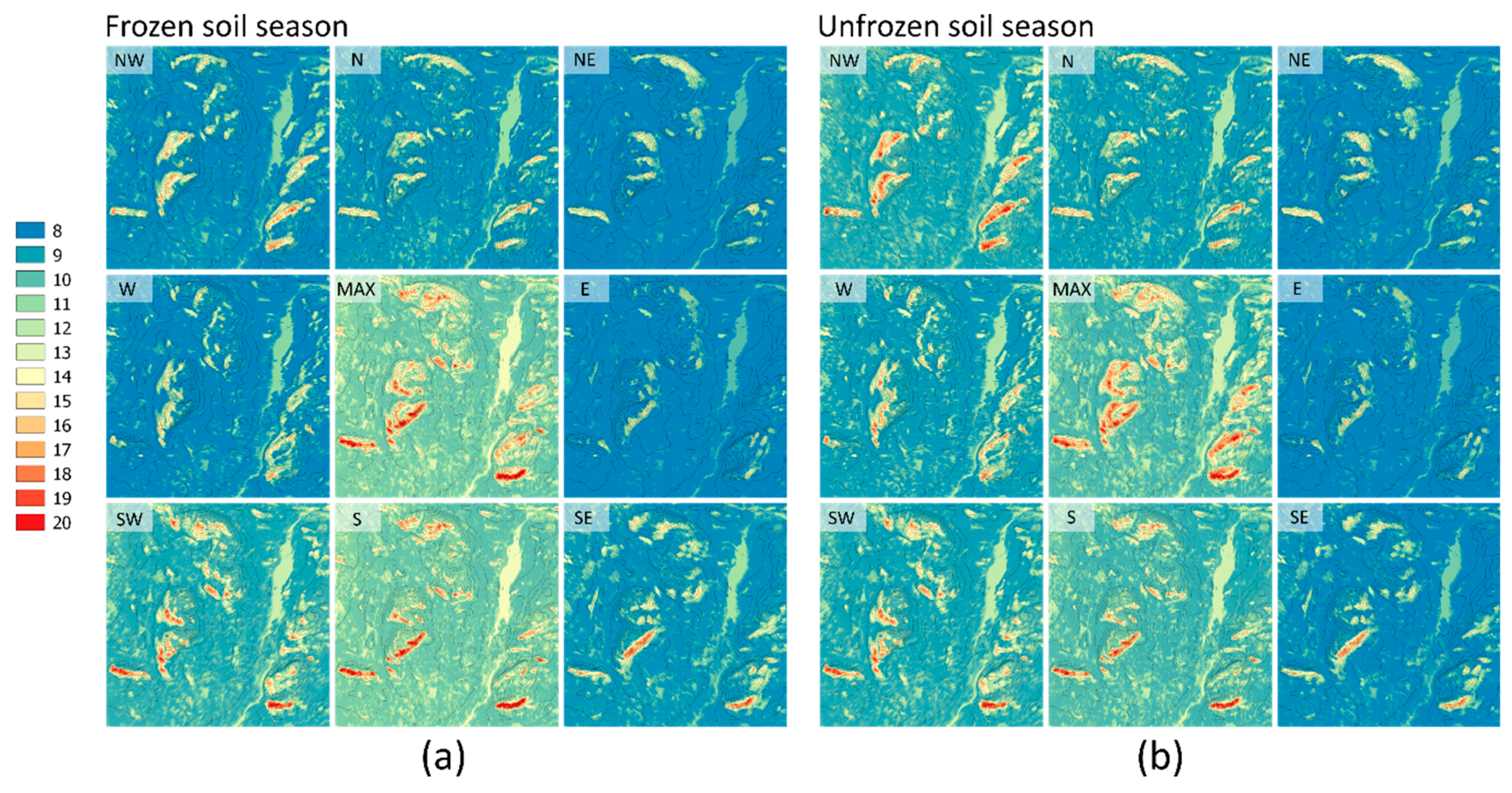
All in all, large-scale differences were in general quite subtle and/or restricted to few areas. On the other hand, small-scale features were visible in the maps over the whole Finland (Figure 4). In detail, these local scale nuances in the behavior of wind multiplier downscaled return levels of 10-year maximum wind speeds are demonstrated, only for PP in this study, on 30 × 30 km area from northern Finland with more complex topography (Figure 1b) including multiple hills/fells with elevation changing between 40 and 270 m above sea level.
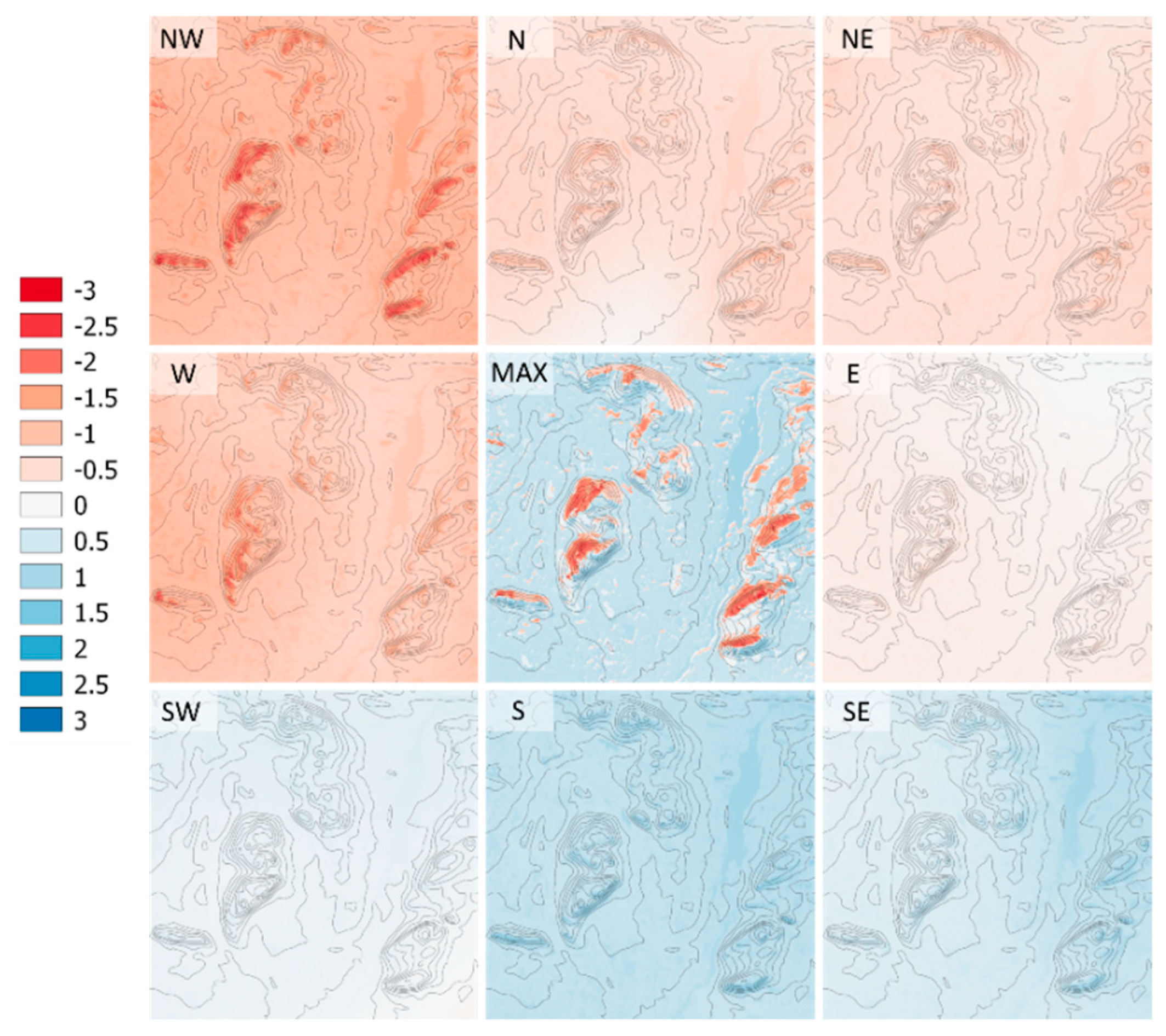
In the example area (Figure 1) used for more detailed analysis about the effects of wind multiplier downscaling, the strongest winds were from the south (Figure 5). This dictates the general large-scale characteristics of aggregated differences (Figure 6, middle), i.e., difference was positive on the majority of the study area. However, generally weaker winds from NW (Figure 5) also had a significant role when the effect of topography was taken into account via wind multipliers. As winds from NW were conversely stronger during unfrozen soil season, this together with relatively strong topographical forcing created isolated areas on hillsides where wind speed return level characteristics are deviating quite a lot from the general conditions of the area (Figure 6, middle). In this example case, stronger winds occurred during soil frost season, but there were also areas, mainly northwestern hillsides, where the situation was opposite.
3.4. Comparison of the 10-Year Return levels of Maximum Wind Speed between OBS vs. ERA and WM
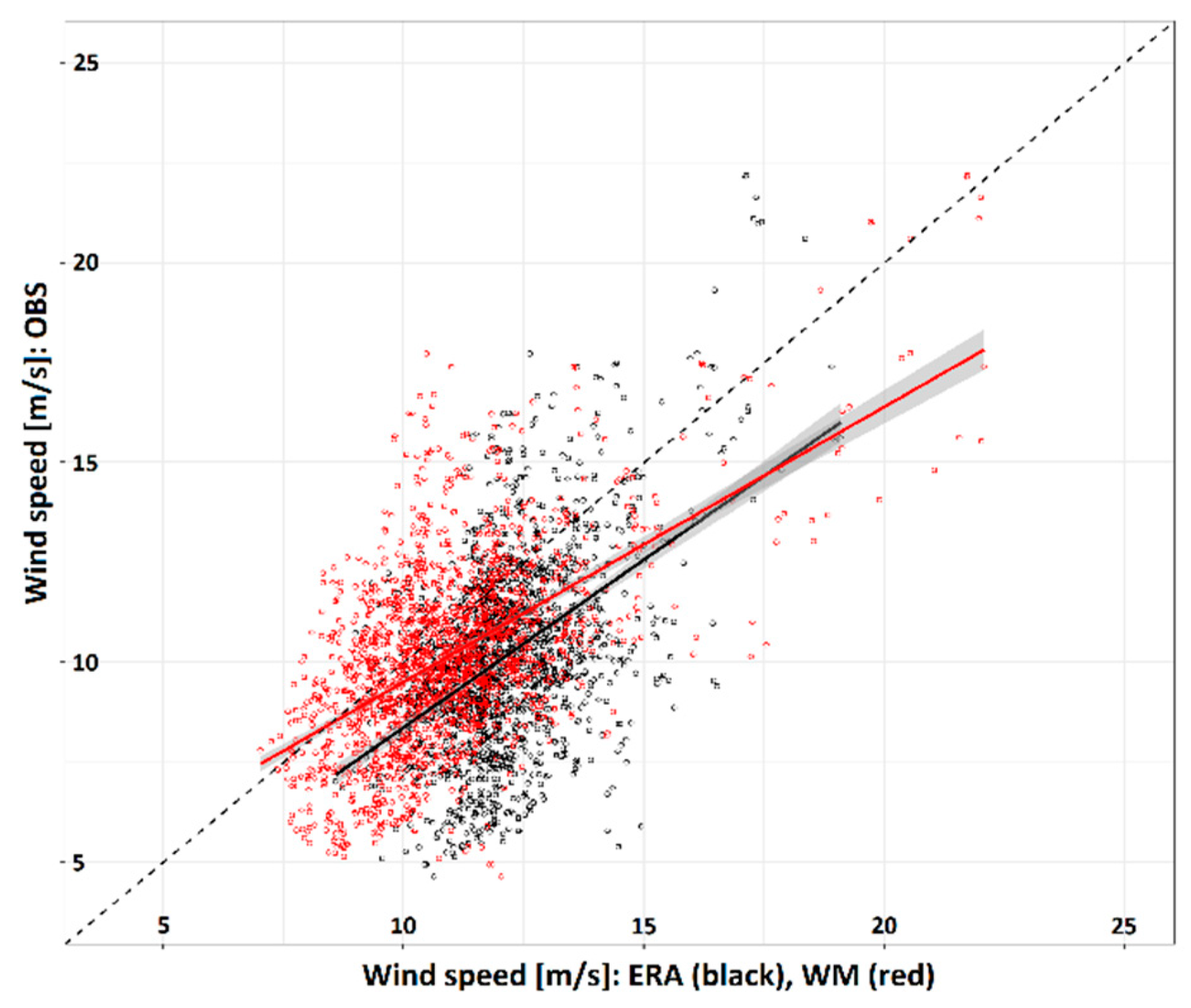
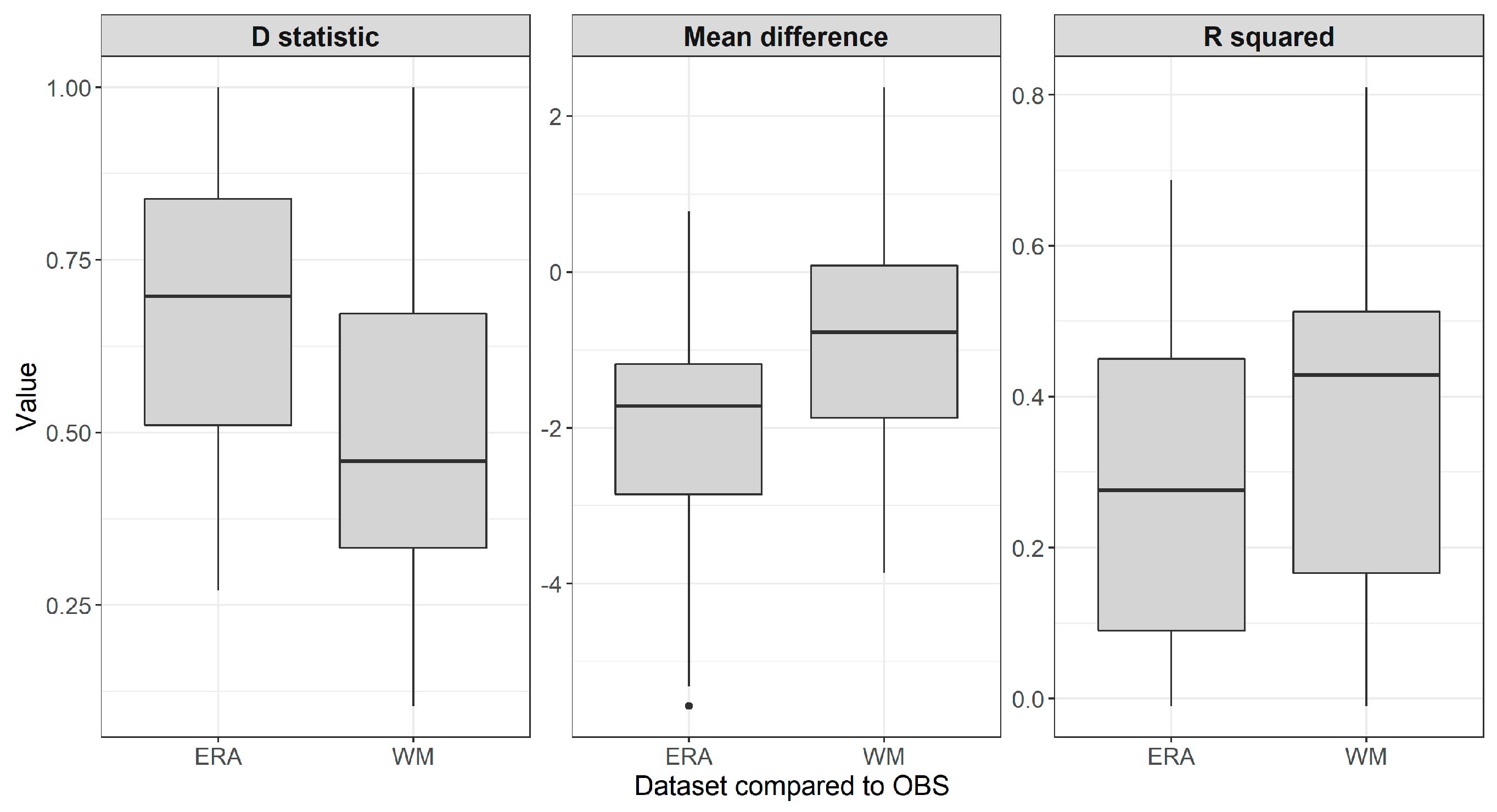
Figure 7 show that even if there is still large variability and some systematic biases, the majority of the OBS and WM comparisons are closer to 1:1 line than the corresponding OBS and ERA comparisons. Also in Figure 8, all three statistics show improvement when comparing differences between OBS and WM to differences between OBS and ERA. Taken over all the comparisons, the D statistic of two-sample Kolmogorov–Smirnov test is decreasing from 0.543 to 0.195, R2 of the linear regression increasing from 0.228 (95% confidence interval 0.196–0.262) to 0.320 (95% confidence interval 0.286–0.355), and the mean difference decreasing from −1.96 to −0.77 (Mann–Whitney U-test p < 2.2e-16).
At some station locations, the application of wind multipliers led to more biased return levels compared to ones derived straight from the ERA-Interim. When considering all the 40 stations and each of three comparison statistic, 23% of the cases showed deterioration of results. However, for only three of the 40 stations, all three comparisons statistics were worsening (not shown).
A majority of the most pronounced overestimations of WM compared to OBS above return levels of 15 m/s (Figure 7) were from a single station at relatively high altitude combined with a large lake in the direction of the largest overestimations. There was also some similarity in the stations characterized by restricted openness, for which wind multipliers overestimated return levels around 10 m/s. For example, the station producing largest overestimations around return levels of 12–13 m/s was located in the residential area on the top of a hill.
4. Discussion
4.1. Main Findings
In this study, we produced high-resolution results (dataset) of 10-year return levels of maximum wind speed, separately for seasons of frozen and unfrozen soil. This was done by utilizing wind speed data from ERA-Interim reanalysis, modelled soil frost data, and surface roughness and topography-based wind multiplier downscaling. Differences in wind speed return levels between seasons of frozen and unfrozen soil are of interest for practical forestry as frozen soil reduces wind damage risk in terms of uprooting of trees due to stronger tree anchorage, in opposite to unfrozen soil during strong winds. Mapping of the most exposed areas to wind damage risk could also provide support for risk management in forest planning and forestry.
Relatively small differences found in this study between the 10-year return levels of maximum wind speeds during the frozen and unfrozen soil conditions can mainly be explained by the large year-to-year variability in the part of year when the annual maximum wind speeds are occurring. In Finland, maximum annual wind speed is only rarely observed during the warmest season from June to September, and those cases are typically connected to more isolated convective weather events. The period from October to December is characterized by frequent large-scale wind storms, however, in most of Finland, the soil can still be unfrozen. During the coldest season from January onwards, the possibility to have soil frost is largest and the occurrence of high wind speeds is almost as frequent as in October to December period. As a result, datasets from where wind speed return levels were derived for both frozen and unfrozen soil seasons were rather similar in the end, especially for spruce stands on clay or silt soil (CSS) and pine stands on sandy soil (SP). Peat is an efficient insulator and it takes longer cold periods before soil frost penetrates deeper into the soil, explaining the higher return levels of maximum wind speed for the unfrozen period in the case of pine stands on peatlands (PP).
The high resolution of wind multiplier downscaling produces also some fine local scale spatial variation in differences between seasons of soil frost. These differences can be quite large and have different sign in the opposing sides of topographic features like hills, ridgelines etc. Our results revealed that taking into account the impact of terrain variability and wind direction, the occurrence of maximum wind speed can change from frozen to unfrozen soil season.
4.2. Strengths and Limitations of Study Approaches
There are multiple sources of uncertainty in our work due to the combination of results from several modelled datasets, use of statistical estimation approaches and aim to produce high-resolution information for the whole of Finland apart from the archipelago. Uncertainties related to return level estimation are somewhat increased in coastal areas. This applies especially for PP as some of the years have no frost at all, and therefore smaller dataset for return level estimation of wind speed in soil frost season. Generally, uncertainty related to 10-year wind speed return level estimates can be considered to be small (+/−1 m/s).
Also, the use of a single threshold of 20 cm for needed soil frost depth to provide sufficient support for anchorage of trees is a rather large simplification in our approach. In reality, needed soil frost depth is affected by various factors, like e.g., soil type, soil wetness, and tree species and other tree and stand characteristics. Furthermore, in the used soil frost model soil water content is assumed to be constant, therefore not representing the extreme cases of very wet or dry conditions. One rather unnecessary source of uncertainty is our use of modelled snow depth, especially as we restricted our work to the observed climate, with the possibility to use gridded observational datasets presumably having smaller uncertainties. However, our approach is justified as we are planning to take projected climate change into account in future work. In the end, [31] concluded that despite many uncertainties in soil frost modelling; their results were, in general, reasonable.
Unfortunately, point observations from operational weather stations do not provide the best possible basis for the validation of wind multiplier downscaled return levels of maximum wind speeds. Operational weather stations are usually founded on locations representing regional climatic conditions or for practicality reasons on specific locations. E.g., 17 out of 40 stations used here are located within flat and open airports and airfields for purposes of aviation. This, compared to the objective of wind multiplier downscaling, i.e., to take into account the influence of small-scale topographic and surface roughness derived variations in wind speed, does not provide an ideal starting point for validation of our results. This applies especially to our application in forestry, where the interest is focused more on areas where wind damage risk is increased. In fact, considering all 40 stations and each of eight wind directions, wind multiplier values are over 1.0, i.e., increasing the wind speed return level estimate derived from ERA-Interim reanalysis, in only 15% of the cases. More detailed and accurate validation would need a more specified measurement campaign in a more complex terrain, which would also make possible the fine tuning of the wind multiplier method. Still, our validation results indicated that wind multipliers improve the wind speed return levels derived straight from ERA-Interim reanalysis by producing return levels less biased as a whole.
The high-resolution wind speed return levels, taking into account the upwind surface roughness and topography, produced in this study may provide a valuable support for wind damage risk assessment. In wind damage risk assessment it is first calculated the critical wind speed (CWS) needed for wind damage of trees to occur based on different tree and stand properties and forest configurations [27,50,51,52,53], and further on estimated the probability of wind damage and the amount of damage, respectively, based on the probability of CWS see e.g., [52]. Our results could be used e.g., when probabilities of exceeding CWSs are assessed and how these probabilities are affected by the soil frost season.
Despite differences in wind speed return levels between soil frost seasons are small, even statistically non-significant for some forest-soil type combinations and parts of Finland when station level estimates are considered, it should be kept in mind that strong winds occurring during soil frost season are excluded from unfrozen soil season. As there was such a large year-to-year variability in the timing of annual maximum wind speeds, divided surprisingly evenly between soil frost seasons found in this study, return level estimates for both seasons are therefore smaller than ones estimated from annual maximum wind speeds. In this context, differences are expected to increase in the future climate of Finland, as according to [30], the ongoing climate change is expected to reduce frozen soil conditions by several weeks until the end of this century in Finland. This might also lead to more pronounced differences of wind damage risk between different parts of Finland.
5. Conclusions
In this study, we found in general small differences in the 10-year return levels of maximum wind speeds under frozen and unfrozen soil, associated with large variability in the timing of annual maximum wind speeds. On the other hand, larger differences can be expected in the warmer climate. When the soil frost period gets even shorter, there is also a shorter window, and thus smaller probability, for strongest winds to occur in the time of frozen soil.
Further validation of used wind multiplier method could benefit from wind observations measured in a more variable topography compared to observations at operational weather stations used in this study. However, the wind multiplier approach is a pragmatic and computationally feasible way to produce extensive high-resolution dataset to identify local scale areas with elevated wind damage risk compared to regional characteristics. Data produced here is made openly available to promote its further use as a part of a more comprehensive wind damage risk assessment in forest planning and forestry.
Author Contributions
Conceptualization, A.V. and M.L.; methodology, M.L., I.L. and A.V.; software, M.L. and I.L.; formal analysis, M.L. and I.L.; writing—original draft preparation, M.L.; writing—review and editing, M.L., A.V., H.M.P. and I.L.; visualization, M.L. and I.L.; supervision, A.V.; project administration, A.V.; funding acquisition, H.M.P. and A.V.
Funding
This research was supported by the Strategic Research Council of the Academy of Finland (FORBIO project, grant number 314224).
Acknowledgments
We thank Pentti Pirinen for technical support with wind multipliers. We also thank anonymous reviewers for their constructive comments on the manuscript.
Conflicts of Interest
The authors declare no conflict of interest. The funders had no role in the design of the study; in the collection, analyses, or interpretation of data; in the writing of the manuscript, or in the decision to publish the results.
References
- Schelhaas, M.-J.; Nabuurs, G.-J.; Schuck, A. Natural disturbances in the European forests in the 19th and 20th centuries. Glob. Chang. Biol. 2003, 9, 1620–1633. [Google Scholar] [CrossRef]
- Schelhaas, M.-J. Impacts of Natural Disturbances on the Development of European Forest Resources: Application of Model Approaches from Tree and Stand Levels to Large-Scale Scenarios. 2008. Available online: http://edepot.wur.nl/146827 (accessed on 29 April 2019).
- Seidl, R.; Schelhaas, M.-J.; Rammer, W.; Verkerk, P.J. Increasing forest disturbances in Europe and their impact on carbon storage. Nat. Clim. Chang. 2014, 4, 806–810. [Google Scholar] [CrossRef]
- Reyer, C.P.O.; Bathgate, S.; Blennow, K.; Borges, J.G.; Bugmann, H.; Delzon, S.; Faias, S.P.; Garcia-Gonzalo, J.; Gardiner, B.; Gonzalez-Olabarria, J.R.; et al. Are forest disturbances amplifying or canceling out climate change-induced productivity changes in European forests? Environ. Res. Lett. 2017, 12, 034027. [Google Scholar] [CrossRef] [PubMed]
- Gardiner, B.; Blennow, K.; Carnus, J.M.; Fleischner, P.; Ingemarson, F.; Landmann, G.; Lindner, M.; Marzano, M.; Nicoll, B.; Orazio, C.; et al. Destructive Storms in European Forests: Past and Forthcoming Impacts. Final Report to European Commission-DG Environment; European Forestry Institute: Joensuu, Finland, 2010. [Google Scholar]
- Schuck, A.; Schelhaas, M.-J. Storm damage in Europe—An overview. In Living with Storm Damage to Forests; What Science Can Tell Us 3; Gardiner, B., Schuck, A., Schelhaas, M.-J., Orazio, C., Blennow, K., Nicoll, B., Eds.; European Forestry Institute: Joensuu, Finland, 2013; pp. 15–23. [Google Scholar]
- Gregow, H.; Laaksonen, A.; Alper, M.E. Increasing large scale windstorm damage in Western, Central and Northern European forests, 1951–2010. Sci. Rep. 2017, 7, 46397. [Google Scholar] [CrossRef]
- Schelhaas, M.-J.; Hengeveld, G.; Moriondo, M.; Reinds, G.J.; Kundzewicz, Z.W.; ter Maat, H.; Bindi, M. Assessing risk and adaptation options to fires and windstorms in European forestry. Mitig. Adapt. Strateg. Glob. Chang. 2010, 15, 681–701. [Google Scholar] [CrossRef]
- Thom, D.; Seidl, R. Natural disturbance impacts on ecosystem services and biodiversity in temperate and boreal forests. Biol. Rev. 2016, 91, 760–781. [Google Scholar] [CrossRef]
- Kellomäki, S.; Peltola, H.; Nuutinen, T.; Korhonen, K.T.; Strandman, H. Sensitivity of managed boreal forests in Finland to climate change, with implications for adaptive management. Philos. Trans. R. Soc. B 2008, 363, 2341–2351. [Google Scholar] [CrossRef] [PubMed]
- Feser, F.; Barcikowska, M.; Krueger, O.; Schenk, F.; Weisse, R.; Xia, L. Storminess over the North Atlantic and northwestern Europe—A review. Q. J. R. Meteorol. Soc. 2015, 141, 350–382. [Google Scholar] [CrossRef]
- Bärring, L.; von Storch, H. Scandinavian storminess since about 1800. Geophys. Res. Lett. 2004, 31, L20202. [Google Scholar] [CrossRef]
- Bärring, L.; Fortuniak, K. Multi-indices analysis of southern Scandinavian storminess 1780-2005 and links to interdecadal variations in the NW Europe-North Sea region. Int. J. Climatol. 2009, 29, 373–384. [Google Scholar] [CrossRef]
- Brönnimann, S.; Martius, O.; von Waldow, H.; Welker, C.; Luterbacher, J.; Compo, G.P.; Sardeshmukh, P.D.; Usbeck, T. Extreme winds at northern mid-latitudes since 1871. Meteorol. Z. 2012, 21, 13–27. [Google Scholar] [CrossRef]
- Dawkins, L.C.; Stephenson, D.B.; Lockwood, J.F.; Maisey, P.E. The 21st century decline in damaging European windstorms. Nat. Hazards Earth Syst. Sci. 2016, 16, 1999–2007. [Google Scholar] [CrossRef]
- Laapas, M.; Venäläinen, A. Homogenization and trend analysis of monthly mean and maximum wind speed time series in Finland, 1959–2015. Int. J. Climatol. 2017, 37, 4803–4813. [Google Scholar] [CrossRef]
- Vautard, R.; Cattiaux, J.; Yiou, P.; Thépaut, J.-N.; Ciais, P. Northern Hemisphere atmospheric stilling partly attributed to an increase in surface roughness. Nat. Geosci. 2010, 3, 756–761. [Google Scholar] [CrossRef]
- McVicar, T.R.; Roderick, M.L.; Donohue, R.J.; Li, L.T.; Van Niel, T.G.; Thomas, A.; Grieser, J.; Jhajharia, D.; Himri, Y.; Mahowald, N.M.; et al. Global review and synthesis of trends in observed terrestrial near-surface wind speeds: Implications for evaporation. J. Hydrol. 2012, 416–417, 182–205. [Google Scholar] [CrossRef]
- Nikulin, G.; Kjellström, E.; Hansson, U.; Strandberg, G.; Ullerstig, A. Evaluation and future projections of temperature, precipitation and wind extremes over Europe in an ensemble of regional climate simulations. Tellus A 2011, 63, 41–55. [Google Scholar] [CrossRef]
- Pryor, S.C.; Barthelmie, R.J.; Clausen, N.E.; Drews, M.; MacKellar, N.; Kjellström, E. Analyses of possible changes in intense and extreme wind speeds over northern Europe under climate change scenarios. Clim. Dyn. 2012, 38, 189–208. [Google Scholar] [CrossRef]
- Peltola, H.; Kellomäki, S.; Väisänen, H. Model computations of the impact of climatic change on the windthrow risk of trees. Clim. Chang. 1999, 41, 17–36. [Google Scholar] [CrossRef]
- Venäläinen, A.; Tuomenvirta, H.; Heikinheimo, M.; Kellomäki, S.; Peltola, H.; Strandman, H.; Väisänen, H. Impact of climate change on soil frost under snow cover in a forested landscape. Clim. Res. 2001, 17, 63–72. [Google Scholar] [CrossRef]
- Kellomäki, S.; Maajärvi, M.; Strandman, H.; Kilpeläinen, A.; Peltola, H. Change Effects on Snow Cover, Soil Moisture and Soil Frost in the Boreal Conditions over Finland. Silva Fenn. 2010, 44, 213–234. [Google Scholar] [CrossRef]
- Gregow, H.; Peltola, H.; Laapas, M.; Saku, S.; Venäläinen, A. Combined occurrence of wind, snow loading and soil frost with implications for risks to forestry in Finland under the current and changing climatic conditions. Silva Fenn. 2011, 45, 35–54. [Google Scholar] [CrossRef]
- Pirinen, P.; Simola, H.; Aalto, J.; Kaukoranta, J.-P.; Karlsson, P.; Ruuhela, R. Tilastoja suomen Ilmastosta 1981–2010 (Climatological Statistics of Finland 1981–2010); Reports 2012:1; Finnish Meteorological Institute: Helsinki, Finland, 2012. Available online: https://helda.helsinki.fi/handle/10138/35880 (accessed on 28 February 2019).
- Korhonen, J.; Haavanlammi, E. Hydrological Yearbook 2006–2010; Finnish Environment Institute: Helsinki, Finland, 2012. Available online: https://helda.helsinki.fi/handle/10138/38812 (accessed on 28 February 2019).
- Peltola, H.; Kellomäki, S.; Väisänen, H.; Ikonen, V. A mechanistic model for assessing the risk of wind and snow damage to single trees and stands of Scots pine, Norway spruce, and birch. Can. J. For. Res. 1999, 29, 647–661. [Google Scholar] [CrossRef]
- Peltola, H.; Kellomäki, S.; Hassinen, A.; Granander, M. Mechanical stability of Scots pine, Norway spruce and birch: An analysis of tree-pulling experiments in Finland. For. Ecol. Manag. 2000, 135, 143–153. [Google Scholar] [CrossRef]
- Venäläinen, A.; Tuomenvirta, H.; Lahtinen, R.; Heikinheimo, M. The influence of climate warming on soil frost on snow-free surfaces in Finland. Clim. Chang. 2001, 50, 111–128. [Google Scholar] [CrossRef]
- Rankinen, K.; Karvonen, T.; Butterfield, D. A simple model for predicting soil temperature in snow-covered and seasonally frozen soil: Model description and testing. Hydrol. Earth Syst. Sci. 2004, 8, 706–716. [Google Scholar] [CrossRef]
- Lehtonen, I.; Venäläinen, A.; Kämäräinen, M.; Asikainen, A.; Laitila, J.; Anttila, P.; Peltola, H. Projected decrease in wintertime bearing capacity on different forest and soil types in Finland under a warming climate. Hydrol. Earth Syst. Sci. 2019, 23, 1611–1631. [Google Scholar] [CrossRef]
- Dee, D.P.; Uppala, S.M.; Simmons, A.J.; Berrisford, P.; Poli, P.; Kobayashi, S.; Andrae, U.; Balmaseda, M.A.; Balsamo, G.; Bauer, P.; et al. The ERA-Interim reanalysis: Configuration and performance of the data assimilation system. Q. J. R. Meteorol. Soc. 2011, 137, 553–597. [Google Scholar] [CrossRef]
- Etienne, C.; Lehmann, A.; Goyette, S.; Lopez-Moreno, J.-I.; Beniston, M. Spatial Predictions of Extreme Wind Speeds over Switzerland Using Generalized Additive Models. J. Appl. Meteor. Climatol. 2010, 49, 1956–1970. [Google Scholar] [CrossRef]
- Jung, C.; Schindler, D. Statistical Modeling of Near-surface Wind Speed: A Case Study from Baden-Wuerttemberg (Southwest Germany). Austin J. Earth Sci. 2015, 2, 1–11. [Google Scholar]
- Mortensen, N.G. Wind Resource Assessment Using the WAsP Software (DTU Wind Energy E-0135); DTU Wind Energy: Roskilde, Denmark, 2016; Available online: http://orbit.dtu.dk/en/publications/wind-resource-assessment-using-the-wasp-software-dtu-wind-energy-e0135(259e26f3-1828-4e3f-9c37-17de375cd057).html (accessed on 28 February 2019).
- Talkkari, A.; Peltola, H.; Kellomäki, S.; Strandman, H. Integration of component models from the tree, stand and regional levels to assess the risk of wind damage at forest margins. For. Ecol. Manag. 2000, 135, 303–313. [Google Scholar] [CrossRef]
- Zeng, H.; Talkkari, A.; Peltola, H.; Kellomäki, S. A GIS-based decision support system for risk assessment of wind damage in forest management. Environ. Model. Softw. 2007, 22, 1240–1249. [Google Scholar] [CrossRef]
- Schindler, D.; Grebhan, K.; Albrecht, A.; Schönborn, J.; Kohnle, U. GIS-based estimation of the winter storm damage probability in forests: A case study from Baden-Wuerttemberg (Southwest Germany). Int. J. Biometeorol. 2012, 56, 57–69. [Google Scholar] [CrossRef] [PubMed]
- Cechet, R.; Sanabria, L.A.; Divi, C.B.; Thomas, C.; Yang, T.; Arthur, W.C.; Dunford, M.; Nadimpalli, K.; Power, L.; White, C.J.; et al. Climate Futures for Tasmania: Severe wind Hazard and Risk Technical Report; Record 2012/43; Geoscience Australia: Canberra, Australia, 2012.
- Yang, T.; Nadimpalli, K.; Cechet, B. Local Wind Assessment in Australia: Computation Methodology for Wind Multipliers; Record 2014/033; Geoscience Australia: Canberra, Australia, 2014. [CrossRef]
- Venäläinen, A.; Laapas, M.; Pirinen, P.; Horttanainen, M.; Hyvönen, R.; Lehtonen, I.; Junila, P.; Hou, M.; Peltola, H.M. Estimation of the high-spatial-resolution variability in extreme wind speeds for forestry applications. Earth Syst. Dyn. 2017, 8, 529–545. [Google Scholar] [CrossRef]
- Jungqvist, G.; Oni, S.K.; Teutschbein, C.; Futter, M.N. Effect of climate change on soil temperature in Swedish boreal forests. PLoS ONE 2014, 9, e93957. [Google Scholar] [CrossRef] [PubMed]
- Vehviläinen, B. Snow Cover Models in Operational Watershed Forecasting; Publication of the Water and Environment Research Institute 11; National Board of Waters and the Environment: Helsinki, Finland, 1992. Available online: https://helda.helsinki.fi/handle/10138/25706 (accessed on 28 February 2019).
- Aalto, J.; Pirinen, P.; Jylhä, K. New gridded daily climatology of Finland: Permutation-based uncertainty estimates and temporal trends in climate. J. Geophys. Res. Atmos. 2016, 121, 3807–3823. [Google Scholar] [CrossRef]
- Coles, S. An Introduction to Statistical Modeling of Extreme Values; Springer Series in Statistics; Springer: London, UK, 2001. [Google Scholar] [CrossRef]
- Stephenson, A.G. EVD: Extreme Value Distributions. R News 2002, 2, 31–32. [Google Scholar]
- Gilleland, E.; Katz, R.W. extRemes 2.0: An Extreme Value Analysis Package in R. J. Stat. Softw. 2016, 72, 1–39. [Google Scholar] [CrossRef]
- AS/NZS 1170.2: Structural Design Actions, Part 2: Wind Actions, 2nd ed.; Standards Australia International/Standards New Zealand: Sydney, Australia; Wellington, New Zealand, 2011.
- Büttner, G.; Soukup, T.; Kosztra, B. CLC2012: Addendum to CLC2006 Technical Guidelines. 2014. Available online: https://land.copernicus.eu/user-corner/technical-library (accessed on 28 February 2019).
- Peltola, H.; Ikonen, V.; Gregow, H.; Strandman, H.; Kilpeläinen, A.; Venäläinen, A.; Kellomäki, S. Impacts of climate change on timber production and regional risks of wind-induced damage to forests in Finland. For. Ecol. Manag. 2010, 260, 833–845. [Google Scholar] [CrossRef]
- Dupont, S.; Ikonen, V.-P.; Väisänen, H.; Peltola, H. Predicting tree damage in fragmented landscapes using a wind risk model coupled with an airflow model. Can. J. For. Res. 2015, 45, 1065–1076. [Google Scholar] [CrossRef]
- Ikonen, V.-P.; Kilpeläinen, A.; Zubizarreta-Gerendiain, A.; Strandman, H.; Asikainen, A.; Venäläinen, A.; Kaurola, J.; Kangas, J.; Peltola, H. Regional risks of wind damage in Boreal forests under changing management and climate projections. Can. J. For. Res. 2017, 47, 1–45. [Google Scholar] [CrossRef]
- Suvanto, S.; Henttonen, H.M.; Nöjd, P.; Mäkinen, H. High-resolution topographical information improves tree-level storm damage models. Can. J. For. Res. 2018, 48, 721–728. [Google Scholar] [CrossRef]
Figure 1.
(a) Locations of 40 weather stations (black dots), division of the Finland into three parts, and location of detailed study area (square with black borders). (b) Topography and elevation (meters above sea level) of detailed study area.
Figure 1.
(a) Locations of 40 weather stations (black dots), division of the Finland into three parts, and location of detailed study area (square with black borders). (b) Topography and elevation (meters above sea level) of detailed study area.

Figure 2.
Annual mean (top row), maximum (middle row), and minimum (bottom row) number of modelled soil frost days over the period 1979–2014 in three forest and soil types. CSS (spruce on clay/silt), SP (pine on sand), PP (pine on peat).
Figure 2.
Annual mean (top row), maximum (middle row), and minimum (bottom row) number of modelled soil frost days over the period 1979–2014 in three forest and soil types. CSS (spruce on clay/silt), SP (pine on sand), PP (pine on peat).

Figure 3.
(a) Distribution of annual maximum wind speed observation months over 40 weather stations and period 1979–2014. (b) Proportion of annual maximum wind speed (1979–2014) observed either during frozen (black) or unfrozen (grey) soil frost season at weather stations located in southern, central, and northern Finland. CSS (spruce on clay/silt), SP (pine on sand), PP (pine on peat).

Figure 4.
Aggregated maps presenting the maximum of 10-year return level of maximum wind speed [m/s] from cardinal and intercardinal wind directions during season of frozen (left) and unfrozen (middle) soil on: (a) soil type CSS (spruce on clay/silt), (b) SP (pine on sand), and (c) PP (pine on peat). Map on right presents the difference between two seasons (m/s). Distributions present the differences in 10-year return levels between frozen and unfrozen soil seasons wind direction wise, divided into northern (NF, top), central (CF, middle), and southern (SF, bottom) Finland.

Figure 5.
Ten-year return levels of wind speed [m/s] for PP (pine on peat) (a) frozen soil season and (b) unfrozen soil season in the detailed study area of northern Finland (location and topography, see Figure 1). The aggregated maximum values are in the middle, surrounded by the return levels of wind speeds from each of the cardinal and intercardinal directions.

Figure 6.
Differences of values presented in the Figure 5a,b. Positive values correspond to stronger winds during frozen soil season.
Figure 6.
Differences of values presented in the Figure 5a,b. Positive values correspond to stronger winds during frozen soil season.

Figure 7.
Scatterplot comparisons of 10-year return levels of wind speed between OBS and ERA (black) and between OBS and WM (red) at the station locations of 40 weather stations, including eight wind directions, three soil types, and two states of soil frost. OBS stands for return levels derived from observed weather station data, ERA for return levels derived straight from ERA-Interim reanalysis, and WM for ERA-Interim derived return levels downscaled with wind multiplier approach.

Figure 8.
Boxplots of 40 station level comparisons of D statistic of two-sample Kolmogorov–Smirnov test (left), mean differences (middle), and coefficient of determination R2 (right) between return levels derived from observations and ERA-Interim reanalysis (ERA) and between observations and wind multiplier downscaling (WM).

© 2019 by the authors. Licensee MDPI, Basel, Switzerland. This article is an open access article distributed under the terms and conditions of the Creative Commons Attribution (CC BY) license (http://creativecommons.org/licenses/by/4.0/).
Share and Cite
MDPI and ACS Style
Laapas, M.; Lehtonen, I.; Venäläinen, A.; Peltola, H.M. The 10-Year Return Levels of Maximum Wind Speeds under Frozen and Unfrozen Soil Forest Conditions in Finland. Climate 2019, 7, 62. https://0-doi-org.brum.beds.ac.uk/10.3390/cli7050062
AMA Style
Laapas M, Lehtonen I, Venäläinen A, Peltola HM. The 10-Year Return Levels of Maximum Wind Speeds under Frozen and Unfrozen Soil Forest Conditions in Finland. Climate. 2019; 7(5):62. https://0-doi-org.brum.beds.ac.uk/10.3390/cli7050062
Chicago/Turabian StyleLaapas, Mikko, Ilari Lehtonen, Ari Venäläinen, and Heli M. Peltola. 2019. "The 10-Year Return Levels of Maximum Wind Speeds under Frozen and Unfrozen Soil Forest Conditions in Finland" Climate 7, no. 5: 62. https://0-doi-org.brum.beds.ac.uk/10.3390/cli7050062
Note that from the first issue of 2016, this journal uses article numbers instead of page numbers. See further details here.