Determining the Most Sensitive Socioeconomic Parameters for Quantitative Risk Assessment

 ,
,
Abstract
:
1. Introduction and Statement of Problem
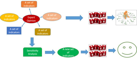
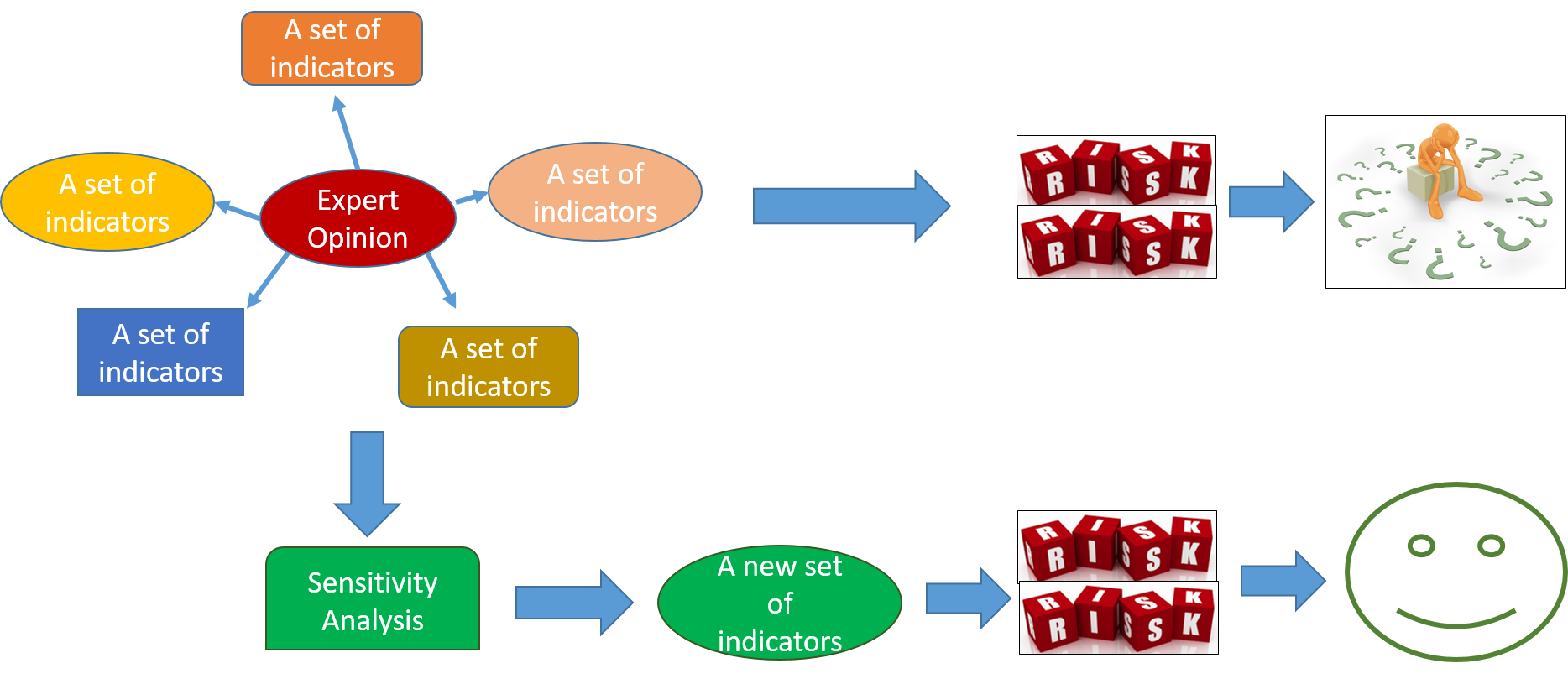
1.1. Overview of the Research
1.2. Research Gap, Research Objectives, and Significance
2. Method
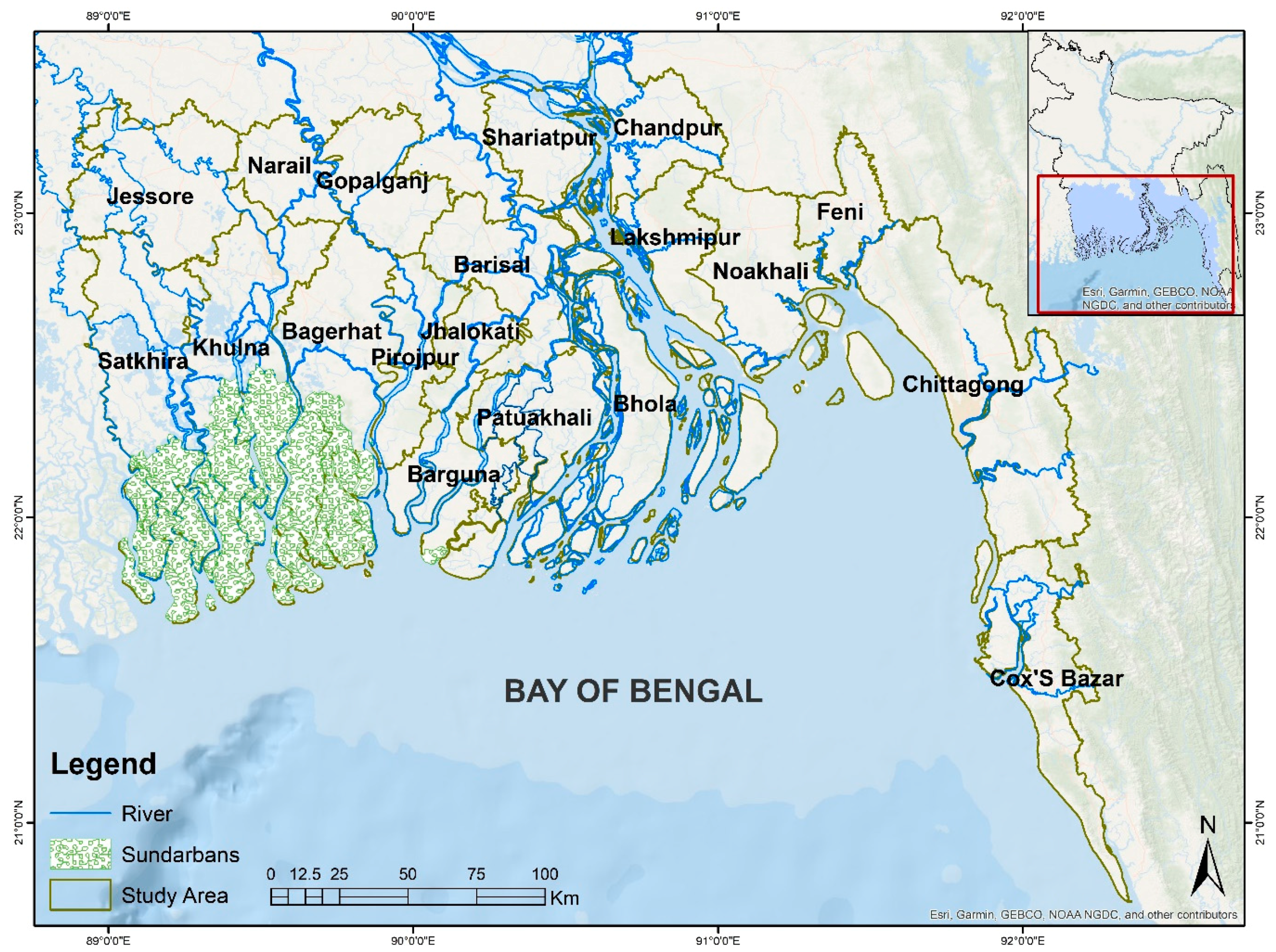
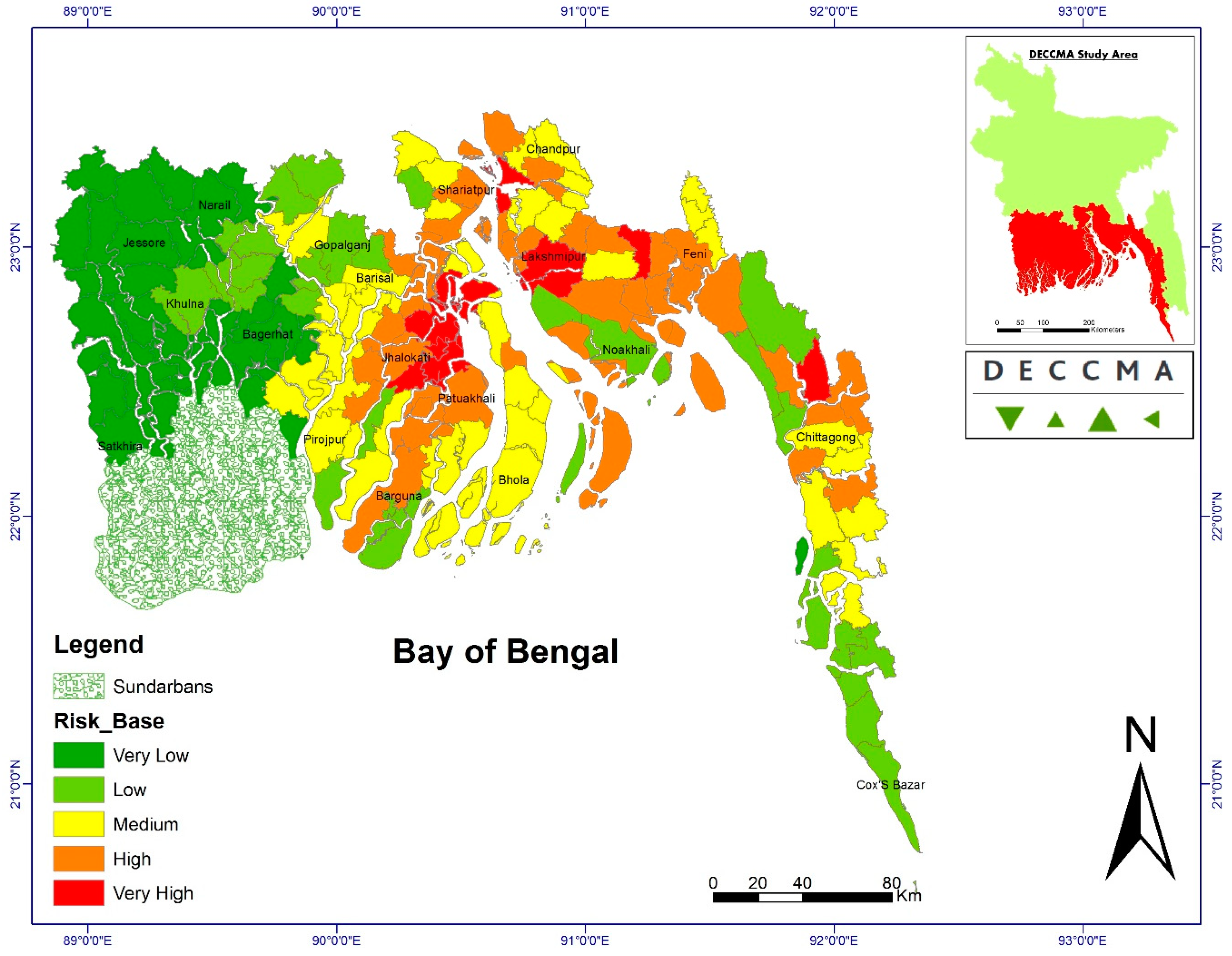
2.1. Study Area Selection
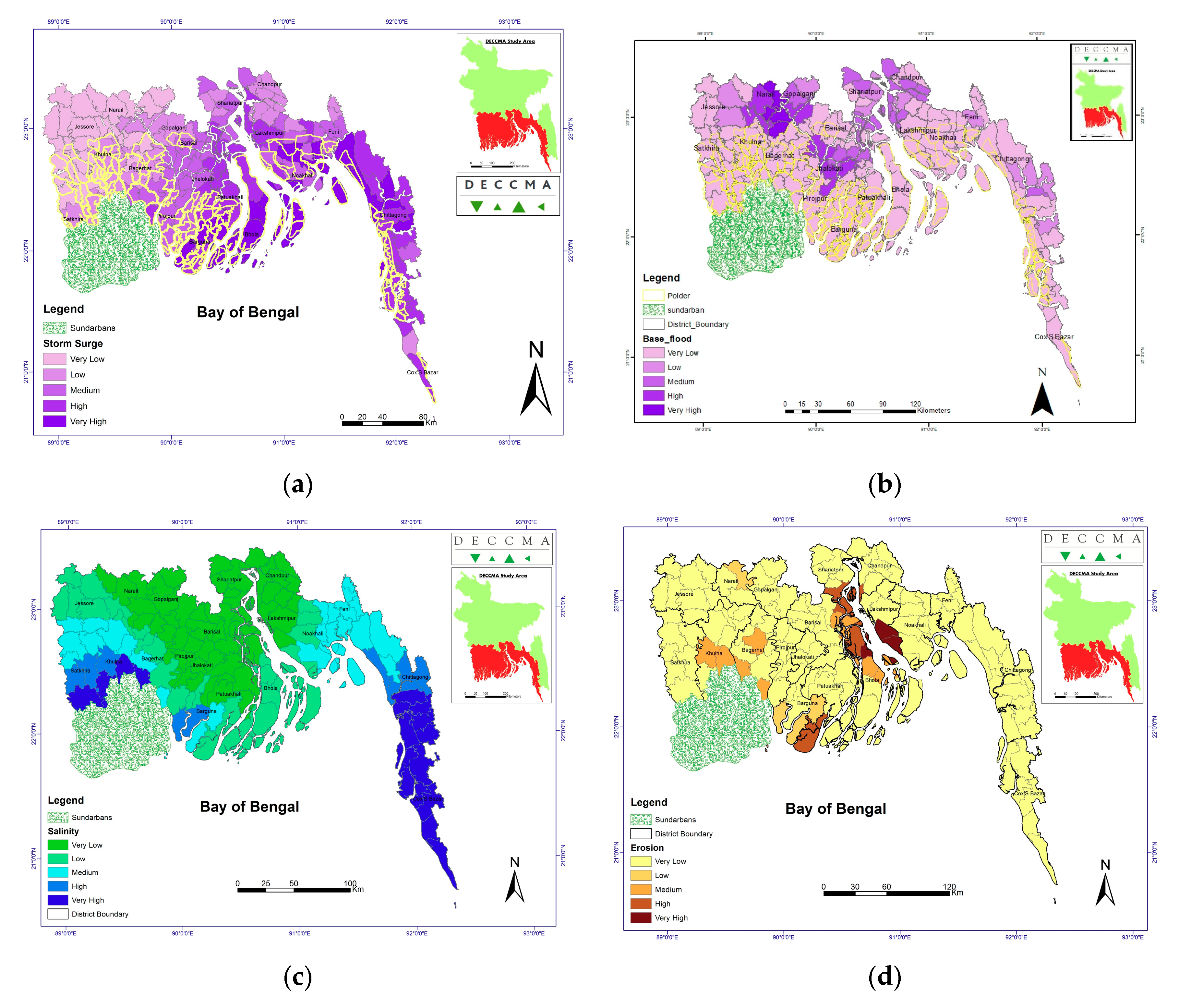
2.2. Hazards in the Study Area
2.3. Available Socioeconomic Indicators to Assess Risk in the Study Area
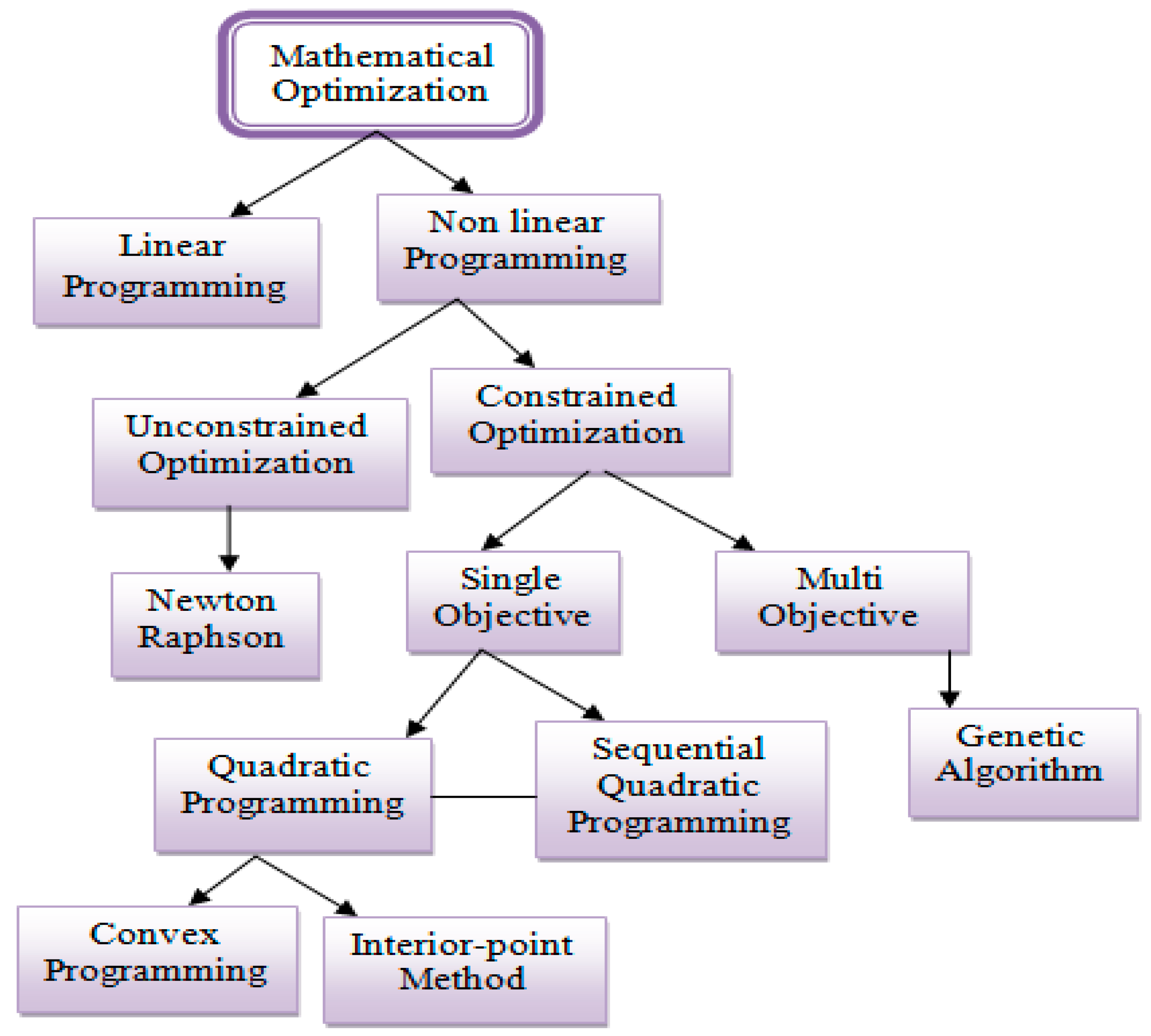
2.4. Non-Linear Programming to Determine the Most Sensitive Indicators
2.4.1. Unconstrained Non-Linear Programming
2.4.2. Constrained Non-Linear Programming
2.5. Development of Non-Linear Programming System
2.6. Solution of Non-Linear Programming System with Karush-Kuhn-Tucker (KKT) Conditions
- (1)
- f(y) is to be feasible to apply the above constraints (iv) and (v).
- (2)
- Gradients of (iii), (iv), and (v) improve objectives and satisfies the following equations:
- (3)
- It satisfies to the positive Lagrangian multiplier .
2.7. Statistical Analysis to Detect Significant Change
3. Results and Discussion
3.1. Selection of the Most Significant Indicators
3.2. Implication of the Most Sensitive Indicators
4. Conclusions and Recommendations
Author Contributions
Funding
Acknowledgments
Conflicts of Interest
References
- UNFCCC. Climate change: Impacts, Vulnerabilities and Adaptation in Developing Countries. Available online: http://unfccc.int/resource/docs/publications/impacts.pdf (accessed on 18 August 2019).
- Krishnamurthy, P.P.; Lewis, K.; Choularton, R.J. A methodological framework for rapidly assessing the impacts of climate risk on national-level food security through a vulnerability index. Glob. Environ. Chang. 2014, 25, 121–132. [Google Scholar] [CrossRef]
- Hahn, M.M.; Riederer, A.A.; Foster, S.S. The livelihood vulnerability index: Apragmatic approach to assessing risks from climate variability and change—A case study in mozambique. Glob. Environ. Chang. 2009, 19, 74–88. [Google Scholar] [CrossRef]
- Bapista, S.R. Design and Use of Composite Indices in Assessments of Climate Change Vulnerability and Resilience; USAID: Washington DC, USA, 2014; Available online: http://www.ciesin.org/documents/Design_Use_of_Composite_Indices.pdf (accessed on 18 August 2019).
- Sullivan, C.; Meigh, J. Targeting attention on local vulnerabilities using an integrated index approach: The example of the climate vulnerability index. Water Sci. Technol. J. Int. Assoc. Water Pollut. Res. 2005, 51, 69–78. [Google Scholar] [CrossRef]
- Smit, B.; Wandel, J. Adaptation, adaptive capacity and vulnerability. Glob. Environ. Chang. 2006, 16, 282–292. [Google Scholar] [CrossRef]
- Cruz, R.R.; Harasawa, H.; Lal, M.; Wu, S.S.A.; Punsalmaa, B.; Honda, Y.; Jafari, M.; Li, C.; Huu Ninh, N. Asia. Climate Change 2007: Impacts, adaptation and vulnerability. In Contribution of Working Group II to the Fourth Assessment Report of the Intergovernmental Panel on Climate Change; van der Linden, P., Parry, M., Canziani, O., Palutikof, J., Hanson, C., Eds.; Cambridge University Press: Cambridge, UK, 2007; pp. 469–506. [Google Scholar]
- Gallopín, G.G. Environmental and sustainability indicators and the concept ofsituational indicators. A system approach. Environ. Model. Assess. 1996, 1, 101–117. [Google Scholar] [CrossRef]
- Downing, T.E.; Butterfield, R.E.; Cohen, S.; Huq, S.; Moss, R.; Raham, A.; Sokona, Y.; Strphen, L. Vulnerability Indices: Climate Change Impacts and Adaptation; Policy Series, 3; UNEP: Nairobi, Kenya, 2001. [Google Scholar]
- Adger, W.N.N.; Brooks, G.; Agnew, B.A.; Eriksen, S. New Indicators of Vulnerability and Adaptive Capacity; Technical Report 7; Tyndall Centre for Climate Change Research: Norwich, UK, 2005. [Google Scholar]
- Brooks, N.; Adger, W.N.; Kelly, P.M. The determinants of vulnerability and adaptive capacity at the national level and the implications for adaptation. Glob. Environ. Chang. 2004, 15, 151–163. [Google Scholar] [CrossRef]
- Vincent, K. Uncertainty in adaptive capacity and the importance of scale. Glob. Environ. Chang. 2007, 17, 12–24. [Google Scholar] [CrossRef]
- Gizachew, L.; Shimelis, A. Analysis and mapping of climate change risk and vulnerability in Central Rift Valley of Ethiopia. Afr. Crop. Sci. J. 2014, 22, 807–818. [Google Scholar]
- Žurovec, O.; Čadro, S.; Sitaula, B.K. Quantitative assessment of vulnerability to climate change in rural municipalities of Bosnia and Herzegovina. Sustainability 2017, 9, 1208. [Google Scholar] [CrossRef]
- Wiréhn, L. Climate Vulnerability Assessment Methodology: Agriculture under Climate Change in the Nordic Region; Linköping University Electronic Press: Linköping, Sweden, 2017; Volume 732. [Google Scholar]
- Eakin, H.; Luers, A.A. Assessing the vulnerability of social-environmental systems. Annu. Rev. Environ. Resour. 2006, 31, 365–394. [Google Scholar] [CrossRef]
- Kocur-Bera, K. Sensitivity Analysis of the Index of a Rural Municipality’s Vulnerability to Losses Resulting from Extreme Weather Events. In Proceedings of the “Environmental Engineering” 10th International Conference, Vilnius Gediminas Technical University, Vilnius, Lithuania, 27–28 April 2017. [Google Scholar]
- Krawczyk, E.; Wrzesińska, J. The use of sensitiveness analysis to the effectiveness’ risk of building and implementation of the cadastre communications system, Zeszyty Naukowe SGGW w Warszawie. Ekonomika i Organizacja Gospo-darki Zywno-ściowej 2009, 74, 111–121. [Google Scholar]
- Tate, E. Social vulnerability indices: A comparative assessment using uncertainty and sensitivity analysis. Nat. Hazards 2012, 63, 325–347. [Google Scholar] [CrossRef]
- Fronzek, S.; Carter, T.T.; Räisänen, J.; Ruokolainen, L.; Luoto, M. Applying probabilistic projections of climate change with impact models: A case study for sub-arctic palsa mires in Fennoscandia. Clim. Chang. 2010, 99, 515–534. [Google Scholar] [CrossRef]
- Saltelli, A.; Nardo, M.; Saisana, M.; Tarantola, S. Composite indicators: the controversy and the way forward. In Statistics, Knowledge and Policy Key Indicators to Inform Decision Making: Key Indicators to Inform Decision Making; OECD Publishing: Paris, France, 2005; pp. 359–372. [Google Scholar]
- Dessai, S.; Hulme, M. Assessing the robustness of adaptation decisions to climate change uncertainties: a case study on water resources management in the East of England. Glob. Environ. Chang. 2007, 17, 59–72. [Google Scholar] [CrossRef]
- Baker, S.; Ponniah, D.; Smith, S. Survey of Risk Management in Major UK Companies. J. Prof. Issues Eng. Educ. Pract. 1999, 125, 94–102. [Google Scholar] [CrossRef]
- Cullen, A.C.; Frey, H.C. Probabilistic Techniques in Exposure Assessment; Plenum Press: New York, NY, USA, 1999. [Google Scholar]
- Nguyen, A.T.; Reiter, S. A performance comparison of sensitivity analysis methods for building energy models. Build. Simul. 2015, 8, 651–664. [Google Scholar] [CrossRef]
- Fiacco, A.V. Sensitivity analysis for nonlinear programming using penalty methods. Math. Program. 1976, 10, 287–311. [Google Scholar] [CrossRef]
- IPCC. Impacts, Adaptation and Vulnerability. Contribution of Working Group II to the Fourth Assessment Report of the Intergovernmental Panel on Climate Change; Canziani, M.L., Palutikof, O.F., van der Linden, J.P., Hanson, P.J., Eds.; Cambridge University Press: Cambridge, UK, 2007; pp. 7–22. [Google Scholar]
- Islam, R. Pre and post tsunami coastal planning and land use policies and issues in Bangladesh. In Proceedings of the Workshop on Coastal Area Planning and Management in Asian Tsunami-Affected Countries, Bangkok, Thailand, 27–29 September 2006. [Google Scholar]
- Bangladesh Bureau of Statistics (BBS). Community Series 2011, Planning Division, Ministry of Planning; Government of the People’s Republic of Bangladesh: Dhaka, Bangladesh, 2011.
- World Bank. Implications of Climate Change on Fresh Groundwater Resources in Coastal Aquifers in Bangladesh. In Agriculture and Rural Development Unit, Sustainable Development Department, South Asia; World Bank: Washington, DC, USA, 2009. [Google Scholar]
- GoB (Government of Bangladesh). State of the Coast; Integrated Coastal Zone Management Program; Ministry of Water Resources and Water Resources Planning Organization: Dhaka, Bangladesh, 2006.
- Dasgupta, S.; Kamal, F.A.; Khan, Z.H.; Choudhury, S.; Nishat, A. River Salinity and Climate Change: Evidence from Coastal Bangladesh, Policy Research Working Paper 6817; World Bank: Washington, DC, USA, 2014. [Google Scholar]
- Bangladesh Bureau of Statistics (BBS), World Bank and World Food Programme. Updating Poverty Maps of Bangladesh; BBS: Dhaka, Bangladesh, 2009.
- Guariguata, M.R.; Cornelius, J.P.; Locatelli, B.; Forner, C.; Sánchez-Azofeifa, G.A. Mitigation needs adaptation: Tropical forestry and climate change. Mitig. Adapt. Strateg. Glob. Chang. 2008, 13, 793–808. [Google Scholar] [CrossRef] [Green Version]
- Holand, I.S. Lifeline Issue in Social Vulnerability Indexing: A Review of Indicators and Discussion of Indicator Application. Nat. Hazards Rev. 2015, 16. [Google Scholar] [CrossRef]
- Haque, A.; Kay, S.; Nichols, R.J. Present and future fluvial, tidal and storm surge flooding in coastal Bangladesh. In Ecosystem Services for Well-Being in Deltas; Nicholls, R.J., Hutton, C.W., Adger, W.N., Hanson, S.E., Rahman, M.M., Eds.; Palgrave Macmillan: London, UK, 2018. [Google Scholar]
- Shamsuddoha, M.; Chowdhury, R.K. Climate Change Impact and Disaster Vulnerabilities in the Coastal Areas of Bangladesh; COAST Trust: Dhaka, Bangladesh, 2007. [Google Scholar]
- Haque, A.; Nichols, R.J. Floods and the Ganges-Brahmaputra-Meghna delta. In Ecosystem Services for Well-Being in Deltas; Nicholls, R.J., Hutton, C.W., Adger, W.N., Hanson, S.E., Rahman, M.M., Eds.; Palgrave Macmillan: London, UK, 2018. [Google Scholar]
- Hiremath, D.B.; Shiyani, R.L. Analysis of Vulnerability Indices in Various Agro-Climatic Zones of Gujarat. Indian J. Agric. Econ. 2013, 68, 122–137. [Google Scholar]
- Wu, J.; Lin, X.; Wang, M.; Peng, J.; Tu, Y. Assessing Agricultural Drought Vulnerability by a VSD Model: A Case Study in Yunnan Province, China. Sustainability 2017, 9, 918. [Google Scholar] [CrossRef]
- Akter, M.; Jahan, M.; Kabir, R.; Karim, D.S.; Haque, A.; Rahman, M. Risk Assessment based on Fuzzy Synthetic Evaluation along Bangladesh Coast. Sci. Total Environ. (Elsevier) 2018, 658, 818–829. [Google Scholar] [CrossRef] [PubMed]
- Soil Resource Development Institute (SRDI). Reconnaissance Soil Survey Reports; Ministry of Agriculture, Government of People’s Republic of Bangladesh: Dhaka, Bangladesh, 2008.
- Armas, I.; Gavris, A. Social vulnerability assessment using spatial multi-criteria analysis (SEVI model) and the Social Vulnerability Index (SoVI model)—A case study for Bucharest, Romania. Nat. Hazards Earth Syst. Sci. 2013, 13, 1481–1499. [Google Scholar] [CrossRef]
- Kabir, R. Determination of critical risk due to storm surges in the coastal zone of Bangladesh. Master’s Thesis, Institute of Water and Flood Management, Bangladesh University of Engineering and Technology, Dhaka, Bangladesh, November 2017. [Google Scholar]
- World Bank. Economics of Adaptation to Climate Change. 2011. Available online: http://www.worldbank.org/en/news/feature/2011/06/06/economics-adaptation-climate-change (accessed on 18 August 2019).
- Toufiqu, K.A.; Mohammad, Y. Vulnerability of Livelihoods in the Coastal Districts of Bangladesh. Bangladesh Dev. Stud. 2013, XXXVI, 95–120. [Google Scholar]
- Hemingway, L.; Priestley, M. Natural hazards, human vulnerability and disabling societies: a disaster for disabled people? Rev. Disabil. Stud. Int. J. 2014, 2. Available online: http://hdl.handle.net/10125/58270 (accessed on 21 August 2019).
- Satterthwaite, D. Climate change and urbanization: Effects and implications for urban governance. In Proceedings of the United Nations Expert Group Meeting on Population Distribution, Urbanization, Internal Migration and Development, DESA, New York, NY, USA, 21–23 January 2008; pp. 21–23. [Google Scholar]
- Nakhooda, S.; Watson, C. Adaptation Finance and the Infrastructure Agenda; Working Paper 437; Overseas Development Institute: London, UK, 2016. [Google Scholar]
- DECCMA. DEltas Vulnerability and Climate Change. 2018. Available online: http://generic.wordpress.soton.ac.uk/deccma/ wp-content/uploads/sites/181/2017/02/online-version_small_Climate-Change-Migration-and-Adaptation-in-DeltasKey-findings-from-the-DECCMA-project.pdf (accessed on 1 January 2019).
- Zanetti, V.B.; Junior, W.; Freitas, D. A Climate Change Vulnerability Index and Case Study in a Brazilian Coastal City. Sustainability 2016, 8, 811. [Google Scholar] [CrossRef]
- CEGIS. Report on Cyclone Shelter Information for Management of Tsunami and Cyclone Preparedness, Centre for Environmental and Geographic Information Services (CEGIS); Ministry of Food and Disaster Management: Dhaka, Bangladesh, 2009.
- Cutter, S.L.; Bryan, J.B.; Lynn, S.W. Social vulnerability to environmental hazards. Soc. Sci. Q. 2003, 84, 242–261. [Google Scholar] [CrossRef]
- Xenarios, S.; Nemes, A.; Golam, W.S.; Sekhar, N.U. Assessing vulnerability to climate change: are communities in flood prone areas in Bangladesh more vulnerable than those in drought-prone areas? Water Resour. Rural Dev. 2017, 7, 19. [Google Scholar] [CrossRef]
- Bruijn, K. Resilience indicators for flood risk management systems of lowland rivers. Int. J. River Basin Manag. 2004, 2, 199–210. [Google Scholar] [CrossRef]
- World Bank. Agriculture Finance & Agriculture Insurance. 2018. Available online: http://www.worldbank.org/en/topic/financialsector/brief/agriculture-finance (accessed on 18 August 2019).
- Paterson, J.; Berry, P.; Ebi, K.; Varangu, L. Health care facilities resilient to climate change impacts. Int. J. Environ. Res. Public Health 2014, 11, 13097–13116. [Google Scholar] [CrossRef]
- Jeong, D.H.; Ziemkiewicz, C.; Ribarsky, W.; Chang, R.; Center, C.V. Understanding Principal Component Analysis Using a Visual Analytics Tool; Charlotte Visualization Center, UNC Charlotte: Charlotte, NC, USA, 2009. [Google Scholar]
- Ruszczyński, A. Nonlinear Optimization; Princeton University Press: Princeton, NJ, USA, 2006; ISBN 978-0691119151. [Google Scholar]
- Emil, G. Optimality Conditions. 2013. Available online: http://www.eng.newcastle.edu.au/eecs/cdsc/books/cce/Slides/ OptimalityConditions.pdf (accessed on 18 August 2019).
- Zuzana, N. The Karush-Kuhn-Tucker Conditions. 2015. Available online: https://www.cs.cmu.edu/~ggordon/10725-F12/slides/16-kkt.pdf (accessed on 18 August 2019).
- Chakravarti, I.M.; Laha, R.G.; Roy, J. Handbook of Methods of Applied Statistics; John Wiley and Sons: Hoboken, NJ, USA, 1967; Volume I, pp. 392–394. [Google Scholar]
- John, C.; Cleveland, W.; Kleiner, B.; Tukey, P. Graphical Methods for Data Analysis; Wadsworth, Inc.: Wadsworth, OH, USA, 1983. [Google Scholar]
- Chatfield, C. The Analysis of Time Series: An. Introduction, 4th ed.; Chapman & Hall: New York, NY, USA, 1989. [Google Scholar]
- Cleveland, W. Elements of Graphing Data; Wadsworth, Inc.: Wadsworth, OH, USA, 1985. [Google Scholar]


| Domain | Indicators | Impact on Risk | Data Source and Data Unit |
|---|---|---|---|
| Exposure | Cropped Area | Negative impact on risk due to its exposure to hazard [39,40]. | Data source: [41]. Data unit: Percentage of Cropped Area per unit of administrative area. |
| Number of Household | Increased number of households causes increased risk [42,43]. | Data source: [29]. Data unit: Percentage of Number of Household per unit of administrative area. | |
| Population Density | Increased population density increases exposed population to risk [43,44]. | Data source: [29]. Data unit: Total number of population per unit of administrative area. | |
| Sensitivity | Female to Male Ratio | Female population are more sensitive to risk than male population. Increased number of female populations increases risk. | Data source: [29]. Data unit: Ratio of female to male population. |
| Poverty Rate | Poor people are sensitive to hazards. So, higher poverty rates are indicative of higher risk due to same hazard. | Data source: [29]. Data unit: Percentage of extreme poor lies below poverty line. | |
| Dependent Population | Dependent population in an area are the women, children, and elderly people. These group of population are considered as less able to adaptation against risk [42,44,45]. | Data source: [29]. Data unit: Percentage of summation of women, children and elderly population to the total population of an administrative unit. | |
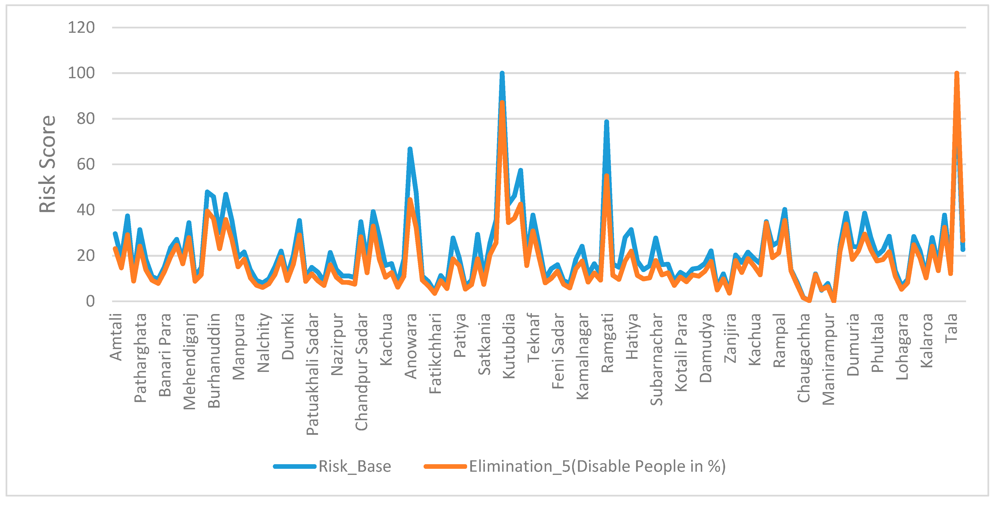
| Disabled People | Physically and mentally disabled people are more sensitive to hazard because of their inability and slow response during a hazard event [46]. | Data source: [29]. Data unit: Percentage of total disabled people to total number of population in an administrative unit. | |
| Unemployed Population | Unemployment decreases the coping capacity and increases the sensitivity and susceptibility to risk [47]. | Data source: [29]. Data unit: Percentage of total unemployed population to total population in an administrative unit. | |
| Adaptive Capacity | Growth center | Growth center is an economic indicator. Increased number of this indicator indicates better economic strength and better adaptive capacity against vulnerability [48]. | Data source: [29]. Data unit: Number of growth center per 5000 of population in an administrative unit. |
| Plantation | Plantation is considered as a buffer against storm surge hazard that reduces the initial thrust of the hazard. Reduction of hazard means reduction of risk [49]. | Data source: [34]. Data unit: Forest area (natural and artificial) per unit of administrative area. | |
| Aquaculture | Shrimp cultivation is the dominant aquaculture in the study area. Aquaculture is considered as an alternative livelihood to adapt against salinity hazard. | Data Source: [34]. Data unit: Shrimp cultivated area per unit of administrative area. | |
| Cyclone shelter | Cyclone shelter is a structural adaptive measure against storm surge hazard. Increased number of cyclone shelter reduces number of human casualty and thus reduces storm surge risk [43,50]. | Data source: [51]. Data unit: Number of cyclone shelter per unit of administrative area. | |
| Cropping intensity | Cropping intensity is an indicator of agricultural activity. Increased cropping intensity means increased adaptive capacity that reduces risk against hazard [39,40,52] | Data source: [41]. Data unit: Percentage of gross cropped area per net cropped area in an administrative unit. | |
| GDP | Gross Domestic Product (GDP) is an economic indicator. Higher GDP means better ability to recover from loss and reduce risk from hazard [53]. | Data source: [29]. Data unit: Gross Domestic Product per capita. | |
| Irrigation Equipment | Shallow tube-well (Stw), Deep tube-well (Dtw), and Low Lift Pump (LLP) are known irrigation equipment in the study area. Increased number of Irrigation Equipment enable a farmer to better adapt with the hazard and thus reduce risk. | Data source: [29]. Data unit: Number of irrigation equipment per unit of cropped land area. | |
| Polder Area | Polder is an encircled embankment constructed to prevent flood in the study area. Increased number of polders reduces flood and thus reduces flood risk [43,54]. | Data source: [34]. Data unit: Percentage of total poldered (embanked) area per administrative unit. | |
| Presence of Lifeline | Lifeline is represented by water supply, sanitation and electricity. Higher number of lifeline utilities are considered to increase adaptive capacity against vulnerability and thus reduces risk [43,44,45]. | Data source: [29]. Data unit: Percentage of tap water and other pond types surface water sources and percentage of connected sanitary and electricity lines per unit area of an administrative unit. | |
| Loan | Loan is considered as the credit facility by co-operative society and banks, particularly to recover from loss due to hazard. Increased loan facilities thus reduce risk due to hazard [55]. | Data source: [29]. Data unit: Percentage of total account holder per total number of populations in an administrative unit. | |
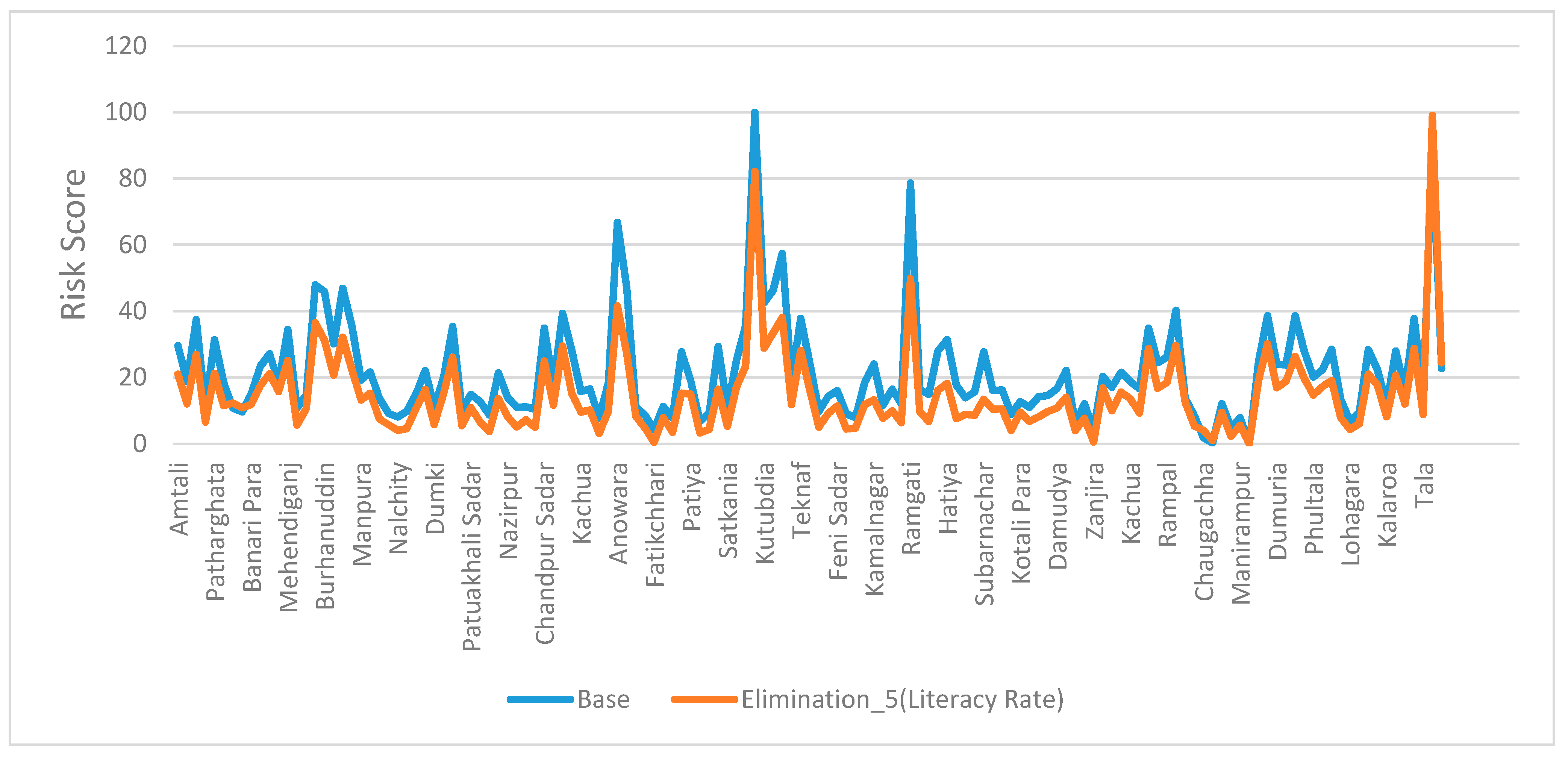
| Literacy Rate | Literate people know better how to adapt with the vulnerability and reduce risk [42,44,45] | Data source: [29]. Data unit: Percentage of number of literate people per unit of administrative area. | |
| Number of Health care Provider | Health care providers play an important role to reduce human casualty during a hazard, which acts to reduce vulnerability and risk of the community [56]. | Data Source: [29]. Data unit: Percentage of health care provider compared to total population in an administrative unit. | |
| Paka and Semi-paka house | Paka and Semi-paka houses represent households which are structurally strong to resist impacts of hazard. Presence of these housing types reduces risk [43,45]. | Data source: [29]. Data unit: Percentage of Paka and Semi-paka houses compared to total number of households in an administrative unit. | |
| Communication Infrastructure | Communication infrastructure is represented by all types of structural measures related to communication. It acts as an adaptive capacity for a community and reduces vulnerability and risk during a hazard [43,44,57]. | Data source: [29]. Data unit: Weighted sum of length of different types of structural measures used for communication purpose in an administrative unit. | |
| Road Density | Increased road density in an area increases the mobility during the time of hazard. This makes it possible to utilize other adaptive measures that reduces risk. | Data source: [29]. Data unit: Total road length in an administrative unit. |
| Indicators | Coefficient of Objective Function | Lower Limit | Upper Limit | Range between Lower Limit and Upper Limit | Rank |
|---|---|---|---|---|---|
| Cropped Area | 0.15901201 | 1.59 × 10⁻¹ | 1.59 × 10⁻¹ | 6.47 × 10⁻⁸ | 1 |
| Number of households | 0.42011697 | 4.20 × 10⁻¹ | 4.20 × 10⁻¹ | 7.27 × 10⁻⁸ | 2 |
| Population density | 0.42087102 | 4.21 × 10⁻¹ | 4.21 × 10⁻¹ | 7.27 × 10⁻⁸ | 3 |
| Cyclone shelter | 0.044980433 | 4.50 × 10⁻² | 6.02 × 10⁻² | 1.52 × 10⁻² | 4 |
| Plantation | 0.046954986 | 4.70 × 10⁻² | 6.29 × 10⁻² | 1.59 × 10⁻² | 5 |
| Polder Area | 0.049170973 | 4.92 × 10⁻² | 6.58 × 10⁻² | 1.66 × 10⁻² | 6 |
| Growth Centre | 0.052033969 | 5.20 × 10⁻² | 6.97 × 10⁻² | 1.76 × 10⁻² | 7 |
| GDP | 0.055189127 | 5.52 × 10⁻² | 7.39 × 10⁻² | 1.87 × 10⁻² | 8 |
| Irrigation Equipment | 0.057194489 | 5.72 × 10⁻² | 7.66 × 10⁻² | 1.94 × 10⁻² | 9 |
| Paka and Semi- paka house | 0.05755829 | 5.76 × 10⁻² | 7.71 × 10⁻² | 1.95 × 10⁻² | 10 |
| Loan | 0.059529224 | 5.95 × 10⁻² | 7.97 × 10⁻² | 2.02 × 10⁻² | 11 |
| Communication Infrastructure | 0.059854204 | 5.99 × 10⁻² | 8.01 × 10⁻² | 2.03 × 10⁻² | 12 |
| Cropping intensity | 0.062339437 | 6.23 × 10⁻² | 8.35 × 10⁻² | 2.11 × 10⁻² | 13 |
| Aquaculture | 0.062434786 | 6.24 × 10⁻² | 8.36 × 10⁻² | 2.12 × 10⁻² | 14 |
| Literacy Rate | 0.063560103 | 6.36 × 10⁻² | 8.51 × 10⁻² | 2.15 × 10⁻² | 15 |
| Number of Health care Providers | 0.063792292 | 6.38 × 10⁻² | 8.54 × 10⁻² | 2.16 × 10⁻² | 16 |
| Presence of Lifeline | 0.066181942 | 6.62 × 10⁻² | 8.86 × 10⁻² | 2.24 × 10⁻² | 17 |
| Road Density | 0.06697054 | 6.70 × 10⁻² | 8.96 × 10⁻² | 2.27 × 10⁻² | 18 |
| Female to male ratio | 0.121988782 | 8.07 × 10⁻² | 1.22 × 10⁻¹ | 4.13 × 10⁻² | 19 |
| Poverty Rate | 0.130673052 | 8.64 × 10⁻² | 1.31 × 10⁻¹ | 4.43 × 10⁻² | 20 |
| Dependent Population | 0.232939206 | 1.54 × 10⁻¹ | 2.33 × 10⁻¹ | 7.86 × 10⁻² | 21 |
| Disabled People | 0.24190139 | 1.60 × 10⁻¹ | 2.42 × 10⁻¹ | 8.20 × 10⁻² | 22 |
| Unemployed population | 0.27249757 | 1.80 × 10⁻¹ | 2.72 × 10⁻¹ | 9.23 × 10⁻² | 23 |
| Indicators | Domain |
|---|---|
| Cropped Area | Exposure |
| Number of households | |
| Population density | |
| Female to male ratio | Sensitivity |
| Poverty Rate | |
| Dependent Population | |
| Disabled People | |
| Unemployed population | |
| Cyclone shelter | Adaptive Capacity |
| Plantation | |
| Polder Area | |
| Growth Centre | |
| GDP | |
| Irrigation Equipment | |
| Paka and Semi-paka house | |
| Loan | |
| Communication Infrastructure | |
| Cropping intensity | |
| Aquaculture | |
| Literacy Rate | |
| Number of Health care Provider | |
| Presence of Lifeline | |
| Road Density |
| Indicators | Domain | |
|---|---|---|
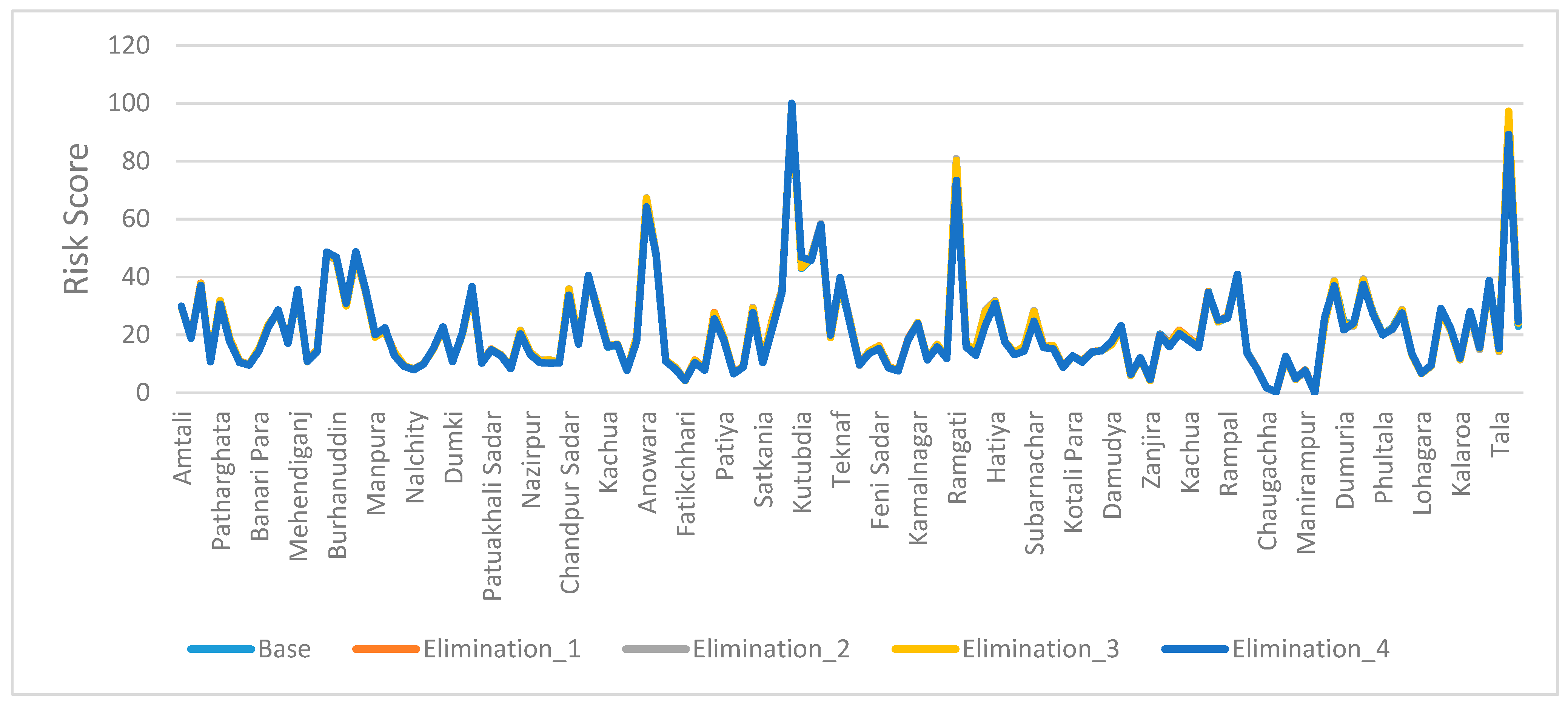
| Elimination_1 | Road Density | Adaptive Capacity |
| Elimination_2 | Presence of Lifeline | |
| Elimination_3 | Number of Health care Provider | |
| Elimination_4 | Unemployed Population | Sensitivity |
| Indicators | |
|---|---|
| Cropped Area | Exposure |
| Number of households | |
| Population density | |
| Cyclone shelter | Adaptive Capacity |
| Plantation | |
| Polder | |
| Growth Centre | |
| GDP | |
| Irrigation Equipment | |
| Paka and Semi-paka house | |
| Loan | |
| Communication Infrastructure | |
| Cropping intensity | |
| Aquaculture | |
| Literacy Rate | |
| Female to male ratio | Sensitivity |
| Poverty Rate | |
| Dependent Population | |
| Disabled People |
© 2019 by the authors. Licensee MDPI, Basel, Switzerland. This article is an open access article distributed under the terms and conditions of the Creative Commons Attribution (CC BY) license (http://creativecommons.org/licenses/by/4.0/).
Share and Cite
Akter, M.; Kabir, R.; Karim, D.S.; Haque, A.; Rahman, M.; Haq, M.A.u.; Jahan, M.; Asik, T.Z. Determining the Most Sensitive Socioeconomic Parameters for Quantitative Risk Assessment. Climate 2019, 7, 107. https://0-doi-org.brum.beds.ac.uk/10.3390/cli7090107
Akter M, Kabir R, Karim DS, Haque A, Rahman M, Haq MAu, Jahan M, Asik TZ. Determining the Most Sensitive Socioeconomic Parameters for Quantitative Risk Assessment. Climate. 2019; 7(9):107. https://0-doi-org.brum.beds.ac.uk/10.3390/cli7090107
Chicago/Turabian StyleAkter, Marin, Rubaiya Kabir, Dewan Sadia Karim, Anisul Haque, Munsur Rahman, Mohammad Asif ul Haq, Momtaz Jahan, and Tansir Zaman Asik. 2019. "Determining the Most Sensitive Socioeconomic Parameters for Quantitative Risk Assessment" Climate 7, no. 9: 107. https://0-doi-org.brum.beds.ac.uk/10.3390/cli7090107