Urban Heat Island in Mediterranean Coastal Cities: The Case of Bari (Italy)


1
Department of Civil, Environmental, Land, Building Engineering and Chemistry, Polytechnic University of Bari, 70125 Bari, Italy
2
School of Environmental Engineering, Technical University of Crete, 73100 Chania, Greece
3
Faculty of Built Environment, University of New South Wales, Sydney 2052, Australia
*
Author to whom correspondence should be addressed.
Climate 2020, 8(6), 79; https://0-doi-org.brum.beds.ac.uk/10.3390/cli8060079
Submission received: 30 April 2020
/
Revised: 14 June 2020
/
Accepted: 18 June 2020
/
Published: 19 June 2020
(This article belongs to the Special Issue The Built Environment in a Changing Climate: Interactions, Challenges and Perspectives)
Abstract
:In being aware that some factors (i.e. increasing pollution levels, Urban Heat Island (UHI), extreme climate events) threaten the quality of life in cities, this paper intends to study the Atmospheric UHI phenomenon in Bari, a Mediterranean coastal city in Southern Italy. An experimental investigation at the micro-scale was conducted to study and quantify the UHI effect by considering several spots in the city to understand how the urban and physical characteristics of these areas modify air temperatures and lead to different UHI configurations. Air temperature data provided by fixed weather stations were first compared to assess the UHI distribution and its daily, monthly, seasonal and annual intensity in five years (from 2014 to 2018) to draw local climate information, and then compared with the relevant national standard. The study has shown that urban characteristics are crucial to the way the UHI phenomenon manifests itself. UHI reaches its maximum intensity in summer and during night-time. The areas with higher density (station 2—Local Climate Zone (LCZ) 2) record high values of UHI intensity both during daytime (4.0 °C) and night-time (4.2 °C). Areas with lower density (station 3—LCZ 5) show high values of UHI during daytime (up to 4.8 °C) and lower values of UHI intensity during night-time (up to 2.8 °C). It has also been confirmed that sea breezes—particularly noticeable in the coastal area—can mitigate temperatures and change the configuration of the UHI. Finally, by analysing the frequency distribution of current and future weather scenarios, up to additional 4 °C of increase of urban air temperature is expected, further increasing the current treats to urban liveability.
1. Introduction
The climate inside cities is heavily influenced by urbanization that radically changes the landscape by replacing open spaces and vegetation with buildings, roads and other infrastructures.
Materials and characteristics of urban surfaces play a fundamental role in the definition of the local climate, together with anthropogenic heat emissions [1]. Therefore, the climate inside the cities is different from that of rural areas. The very well-known phenomenon of Urban Heat Island (UHI) causes an increase in temperature in dense portions of the cities (downtown, in particular) [2]. UHI phenomenon has a direct consequence on the increase in buildings’ energy demand [3,4,5], on energy poverty [6,7], and on people’s health, and on liveability of cities [8,9,10].
Several factors influence UHI. They include the geographical position of the site and weather conditions such as wind speed and cloudiness [11,12]. Moreover, other factors more directly related to human action, such as the alteration of building fabric and pavement properties [13], urban geometry and density, energy production processes are determinant for the UHI phenomenon [14,15]. Among the uncontrollable variables, wind and cloud cover are two primary weather characteristics that affect UHI development, which generally forms during periods of clear skies and calm winds. Conversely, strong winds and cloud cover hinder the formation of the UHI [16].
The climate and topography of cities, primarily determined by their geographical location, also influence the formation of the UHI. For example, the presence of large bodies of water mitigates temperatures due to the sea breeze phenomenon [17]. In coastal cities this phenomenon overlaps with the UHI one, with consequences on local climate [18,19,20,21]. As an example, in the coastal city of Chania (Greece) the UHI reaches its maximum intensity during summer. A strong relation has been demonstrated between UHI and local climate condition. In particular the formation of UHI is strongly influenced by wind speed and direction [22]. Another study conducted in the city of Barcelona (Spain) has shown that in summer, due to the sea breeze effect, the UHI intensity is weaker. As a consequence, the maximum UHI intensity is reached in December [23].
Trees and vegetation also contribute to mitigating temperature increases. The loss of vegetation, together with the presence of impermeable surfaces reduces the evapotranspiration of water, with the consequent increase in surface and air temperatures. Geletič et al. [24] performed a study to analyse the seasonal variability of the Surface Urban Heat Island (SUHI) in three European cities using remote sensing data. The study showed that SUHI differences were more pronounced in summer and that the greatest impact on seasonal variability of SUHI occurred in areas with taller plants.
Urban geometry is another factor that influences UHI development. Urban geometry affects wind flow, energy absorption, and the ability of a given surface to emit long-wave radiation back to space. In urban canyons (i.e., relatively narrow streets lined by tall buildings) [17], during the day, the presence of tall buildings creates shade and thus reduces surface and air temperatures. When the sunlight reaches the surfaces in the canyon, the solar energy is reflected and absorbed by the walls of buildings, creating an increase in temperatures [25]. During the night, buildings and structures can obstruct the heat that is released from urban infrastructures, and urban canyons usually impede cooling. Salvati et al. performed a comparative study of the effects of urban textures on the microclimate in two Mediterranean cities [26]. Five variables (urban morphology, vegetative cover, anthropogenic heat deriving from buildings and traffic and albedo) were considered and related to the variability of the Urban Heat Island Intensity (UHII). The study showed that urban morphology is the variable with the highest impact on UHI phenomenon. A compact urban texture leads to higher UHII because it favours the accumulation of anthropogenic heat in the canopy layer. Moreover, a morphology with higher density causes an increase in temperatures at night, because of the reduction in long-wave radiation losses, due to the lower sky view factor. The findings of Salvati et al. are also confirmed by the results of the study carried out by Paramita et al. in tropical regions [27]. In this case, the additional effect of urban canyons consists of the limitation of wind flows with the consequence increase in both air temperature and relative humidity.
Finally, the microclimate of cities is affected by anthropogenic heat. The intensity of anthropogenic heat emissions varies depending on urban activity and infrastructure [28]. In contrast to what happens in rural areas and in summer, anthropogenic heat can contribute significantly to the development of UHI in winter [29,30].
The present study aims at analysing the urban climate of a coastal Mediterranean city, affected at the same time by the UHI phenomenon and by diurnal sea breeze and nocturnal land-breeze. From this perspective, we have focused the study on the city of Bari (Italy). The analyses presented in this paper are conducted within the Urban Canopy Layer [31], approximatively equivalent to that of the mean height of the main roughness elements (buildings and trees) [32]. Air temperature values recorded in the period between January 2014 and December 2018 at four meteorological stations positioned at ground level (with instruments placed between 2 and 5 m above the ground) are considered. The objective of the study is the assessment of the influence of both phenomena on the modification of the local climate. From this perspective, together with a detailed assessment of extent of the UHI phenomenon in different locations within the city of Bari, a comparison of microclimatic data with the ones included in relevant national standard for the Italian territory [33] is presented. Moreover, an assessment of the impact of UHI in future weather scenarios is presented.
2. Materials and Methods
The study was carried out in the city of Bari (Puglia, Italy 41.12 N, 16.87 E), located on the south-western coast of the Adriatic Sea. The city has a medium density and hosts about 320.000 inhabitants [34]. Bari is a typical Mediterranean city with mild winters and hot summers. The highest temperatures are recorded in August (daily Tavg 24.3 °C) while the lowest ones are in January (daily Tavg 8.7 °C). On average, there are four days of frost per year and 31 days per year with a maximum temperature equal to or greater than 30 °C. During the period when heat stress is most likely to occur, the highest temperatures are concentrated between 12:00 and 14:00. Average annual rainfall is 563 mm, distributed over 70 days on average, with minimum value in summer, maximum peak in autumn and secondary maximum in winter. November is the wettest month and July the driest. The recorded annual average relative humidity is 71.3% with a minimum of 65% in July and a maximum of 77% in November and December [35].
The analyses presented in this paper have been performed within the Urban Canopy Layer and based on the air temperature data recorded by four fixed meteorological stations located in the metropolitan area. Starting from the hourly temperature data, daily, monthly, seasonal and annual variability of the UHI phenomenon has been studied.
The first step to analyse this phenomenon thus consists of identifying two reference points: an urban and a non-urban (or rural) one. In principle, it would be simple to identify the urban point by making it coincide with the core of a city, for instance. On the contrary, the non-urban point is harder to identify. This occurs because, in the same city, the possible factors that contribute to the increase in temperature are many and differently distributed across the urban area. Thus, although considering the same city, it is possible to identify intermediate areas, more or less urbanized than others or more or less rural than others, which make it possible to better understand how geometric, climatic, environmental variations in the urban structure, in the urban landscape are decisive in affecting temperature variations. Consequently, for this study, the concept of the non-urban area was further extended. A preliminary analysis of the area of Bari and its province was carried out by considering several areas (each one monitored with a standard weather station) to understand how the characteristics of the areas might affect temperatures and, therefore, UHI phenomenon. This analysis is essential to identify the reference weather station, used for calculating the Urban Heat Island Intensity (UHII).
Identification of Locations for Weather Stations and Meteorological Data Collection
In order to assess the UHI phenomenon in the city of Bari, a first screening of all available weather stations was performed. While selecting the weather stations in the area, it was found that many of them were located on the roofs of buildings. This specific position of the sensors makes them—and their recorded data—more sensitive to the sea breeze phenomenon, due to the absence of obstacles [23]. Moreover, since the sensors may be too close to outdoor air conditioning equipment, data recording reliability might be affected. Therefore, we considered only the weather stations positioned at the street level. Moreover, to allow for a more precise and complete analysis, all the meteorological stations that missed more than a month of recorded data during the investigated years were excluded. Therefore, a total of four weather stations located in the metropolitan city of Bari have been considered. Three weather stations are located in the city of Bari (Figure 1a). They are all managed by the regional environmental protection agency (Agenzia Regionale per la Prevenzione e la Protezione dell’Ambiente - ARPA Puglia) [36]. One weather station is located in the city of Valenzano (Figure 1b), and is managed by the Mediterranean Agronomic Institute (Centre International de Hautes Études Agronomiques Méditerranéennes - CIHEAM) of Bari [37].
Figure 2 includes the exact location and an aerial image of each site, while Figure 3 shows a detailed image of the weather stations.
Stations 1, 2 and 3 were installed between 2004 and 2012 to monitor the air quality in the area. They detect the presence of pollutants such as CO, C6H6, PM10, NO2, PM2.5 and record climatic data such as air temperature, relative humidity, wind speed and direction, solar radiation, atmospheric pressure and precipitation. Station 4 has been active since 1983 and has been installed for scientific and educational purposes. It records only climatic data, the same as for previous stations.
Weather station 1 is positioned along the promenade Lungomare Starita, in an area next to the sea where the university sport centre is located. It is a non-residential area, not restricted by obstacles such as relatively tall or low buildings and not on direct urban traffic. The values of geometric and surface cover properties (see Table 1) calculated for a squared area (side of 600m) centred on the weather station allow us to classify the zone as Local Climate Zone (LCZ) 9 (sparsely built), according to the local climate zone classification by Stewart and Oke (2012) [38]. Given that the station is positioned near the sea, subclass G—water—is added. Weather station 2 is placed in the city centre, in an area with high population density, and mid-rise residential buildings. The building blocks, very close one to each other, are interspersed with narrow streets, not exceeding 15 m in width. Together they create a very dense square mesh, interrupted by the main street—Corso Cavour—where the weather station is located. Apart from the presence of trees along the main street, the area has no special and significant green spaces. According to the local climate zone classification, the area can be defined as LCZ 2—compact mid-rise. Weather station 3 is located in a predominantly residential area, close to the city centre. Various green spaces are also present. According to the local climate zone classification, the area can be defined as LCZ 5—open mid-rise. Finally, weather station 4 is located 10 km far from the city centre, on agricultural land owned by the CIHEAM. The station is, thus, located in a traffic-free area, free from obstacles and surrounded by sparse buildings not higher than three storeys above ground. According to the local climate zone classification, station 4 belongs to the same climate zone as station 1 (LCZ 9—sparsely built), but with a different subclass (B—scattered trees).
According to the objectives of our study, among all the provided data, it was decided to consider a timeframe of five years for the analyses. From this perspective, five available consecutive years, from January 2014 to December 2018, were considered. During this timeframe, not all data were provided by the weather stations. In these cases, it was decided not to fill the data gaps since any assumption or approximation of data would have meant attributing arbitrary values. Table 2 includes the percentages of missing hourly air temperature data for each control unit and for each year.
Moreover, data cleaning and validation was performed. From a first analysis of the data, some values were not consistent or realistic (for example, one order of magnitude higher than the values of the previous or following hour). This required a manual adjustment of the data to reduce the error probability in the subsequent analyses. The performed adjustment was not numerical, as the figures were not modified. We simply moved one or two decimal points to make the data consistent with the previous or subsequent data.
3. Results
3.1. UHI in Bari: Meteorological Data Collection and Comparison
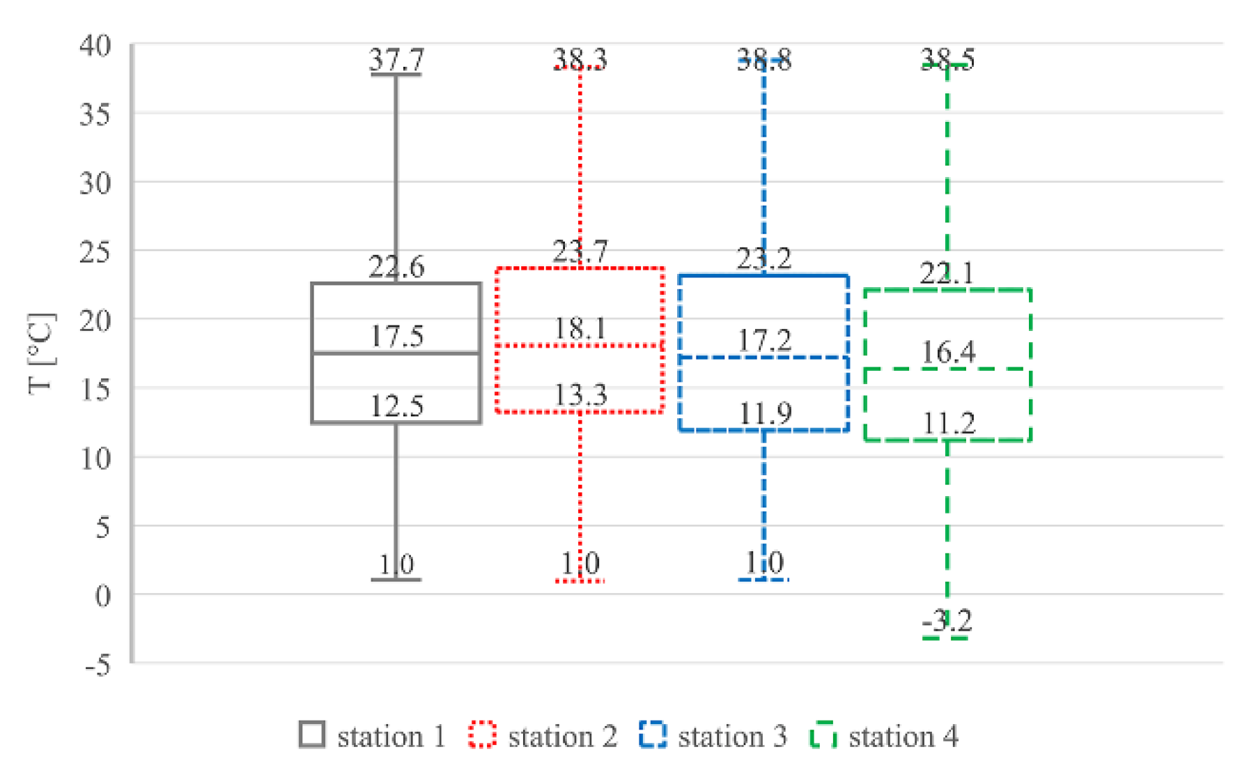
A first analysis involves the identification of the hourly variation patterns of air temperatures in the four stations. By aggregating all data recorded at the four stations during the five years, it has been possible to perform a statistical analysis of hourly temperatures recorded at the four stations, which is summarized in Figure 4. It can be highlighted that station 2 is the one recording the highest average values of air temperatures (18.1 °C), followed by station 1 (17.5 °C) and station 3 (17.2 °C), while station 4 is the one recording the lowest average hourly temperatures (16.4 °C). Station 3 is the one recording the absolute highest temperature (38.8 °C), while station 4 is the one recording the absolute lowest temperature (−3.2 °C). All the three stations placed in Bari have recorded during the five years of measurements hourly temperature values always above 0 °C. Furthermore, from the box plot, it can be recognized that station 3 presents the highest dispersion of values (difference between the first and third quartile of values of 11.3 °C), while station 1 recorded less dispersed values (difference between the first and third quartile of 10.1 °C).
Therefore, it was decided that we would deepen the hourly analysis, by plotting the hourly data of air temperature during the hottest (August) and coldest (December) months for the five years of the study, as shown in Figure 5. In August, during daytime, the highest temperatures generally seem to be those recorded by station 4 in 2014 and 2018, and by station 3 in 2015-2016-2017. During night hours, station 2, in all 5 years, is the one with the highest temperatures, followed by stations 3, 1 and 4 in 2014-2017-2018, and stations 1, 3 and 4 in 2015 and 2016.
Analysing the graphs for December, during the daytime the highest temperatures remain those recorded by station 3 in 2014 and 2015. In 2016, the temperatures recorded by station 1 are higher in the first half of the month, those of station 3 in second half of the month. In 2017, station 2 records the highest daytime temperatures, while in 2018 it is station 1. With reference to the night hours, the situation is like that of August. However, in 2018, temperatures recorded at station 1 are higher, even at night.
By the analysis of the data presented in Figure 5, it is interesting to consider the patterns of temperatures recorded at weather station 1 (i.e., the one located near the sea). During the heatwave of August 2018, it can be observed that the temperatures recorded at weather station 1 are rather low compared with the previous years and with the temperatures of the other weather stations for the same year. This happens also when data are compared with the ones obtained from weather station 4, which generally records the lowest temperatures. A maximum temperature at station 1 of 28.3 °C (11 August 2018) is reached, while the temperature recorded at stations 2, 3, and 4 are, respectively, 32.8 °C (13 August 2018), 34.7 °C (11 August 2018), and 33.6 °C (8 August 2018). Moreover, the temperature peaks at station 1 are considerably lower, and the trend of maximum temperatures is more constant. This can be accounted for by the sea breeze phenomenon [21].
Figure 6 summarizes the average, maximum, and minimum monthly temperatures for each location and for the five years considered. In 2014, although with a difference of some degrees in winter (December, January, and February) where higher temperatures are recorded at station 1, in summer (between May and September), averages are roughly similar for the four stations. In the subsequent years, the minimum, maximum, and average monthly temperatures are quite distinguishable, and they rarely overlap. In general, the monthly average temperatures calculated at stations 1 and 4 remain lower than those calculated for values recorded at stations 2 and 3, with differences that may even exceed 2 °C in summer and winter. This is particularly evident in the years 2017 and 2018, and precisely in 2018, when the abnormal decrease in temperature for station 1 is observed and is mainly due to the sea breeze phenomenon.
Looking at the patterns of maximum monthly temperatures, stations 3 and 4 show the highest values during the months from April to August. During the other months and, in particular, in the coldest ones, the maximum temperatures recorded by all the weather stations have values similar one to each other. As previously described, only in 2014 did the monthly maximum temperature values show a relatively small variation for the four weather stations considered.
As far as minimum temperatures are concerned, station 2 is the one that records the highest values, both in the hot and cold months. It must be noted that the minimum temperature difference between station 2 and the other stations is particularly pronounced in the cold months, from November to March.
3.2. Definition of Reference Station and Determination of Urban Heat Island Intensity
The analysis of temperatures included in the previous paragraph shows that the UHI phenomenon is present in the area considered. Therefore, in this paragraph, the classical indicator to quantitatively describe UHI effect, the Urban Heat Island Intensity (UHII), is analysed. The study illustrated in the previous paragraph was meant to understand and quantify more accurately, on the basis of air temperature data, how important the Heat Island effect is in the considered area in order to define the area where such a phenomenon is less pronounced and so as to identify the reference non-urban area.
The reference station must be selected where there is a low influence of buildings (i.e., in a flat area with high amount of vegetation). Moreover, since the influence of the wind regime is particularly relevant in the definition of the UHI phenomenon [39], for coastal cities, it is suggested that we consider a reference station at a similar distance from the coastline than the urban area under consideration [40]. In previous studies conducted in coastal cities, either airport stations [41,42] or non-urban stations located along the coastline [43,44,45] were selected. For all of these reasons, we had to exclude station 4 from the assessment of UHII. Therefore, among the three remaining stations, station 1 is the one that exhibits the characteristics of the non-urban area as previously defined, and therefore, has been considered as the reference station.
Consequently, several analyses on the UHII were assessed by considering:
- monthly average temperatures (UHIIm) and annual average temperature (UHIIy);
- average daily temperatures (UHIId);
- maximum hourly difference of temperature recorded during each day (UHIImax);
- diurnal (UHIIday) and nocturnal (UHIInight) urban heat island intensity;
The following Table 3 and Table 4 include the results of the analyses conducted, respectively, on the monthly (and annual average) and daily temperatures. In Table 3, it can be recognized a missing value for January 2017, as during that month the reference station did not record any value. For all the other analyses, any missing data for one weather station (hourly or daily), were not considered in the average also for the other weather stations, as to make the averages more consistent by using the same number of data.
Analysing the data included in Table 4, it can be observed that UHII is generally higher at weather station 2 than at weather station 3. The maximum UHII values based on average yearly data are, respectively, 2 °C and 1 °C for stations 2 and 3 and are both recorded in 2018. On a monthly basis, the highest UHII is also recorded in 2018, with both stations recoding in June monthly average temperature values 6.6 °C higher than the ones recorded at the reference station. From the analysis of the data, it can also be observed that for three out of five years (2015, 2017 and 2018), the maximum monthly UHII is observed in June. For station 2, it is also common to find maximum UHI intensities during cold months (March 2014 and January 2016), while for station 3 in 2014 and 2016, the maximum monthly UHII is found in hot months (August 2014 and July 2016).
Analysing the results included in Table 4, the comparison the daily temperature differences confirms what is observed from the annual analysis. In fact, by analysing the maximum daily UHII for each year, the intensity calculated at station 2 is higher than the one calculated at station 3.
The highest intensity for both areas is recorded in 2018 and is equal to 5.5 °C for station 2, 1.3 °C higher than at station 3 on the same day (23 March 2018) and 4.6 °C for station 3, slightly higher by 0.3 °C than at station 2 on that same day (2 July 2018). Such a high difference may be correlated with the presence of the heatwave of that year, and with the fact that, as previously explained, the sea breeze effect has caused the temperatures of the reference weather station (station 1) to drop. The calculated average values were accordingly higher. In 2014, the UHII at station 2 is more than double that at station 3 on 3 December 2014, whereas on 23 May 2014, station 2 exhibits higher intensity with a difference of 0.3 °C compared to station 3. In 2015 and in 2016, the highest intensity for both the areas is recorded on the same day: 19 May 2015 and 13 July 2016. In 2015, the intensity calculated at station 2 is 0.5 °C higher than the one calculated at station 3, whereas in 2016, it reverses. This phenomenon may depend on many factors that act individually or simultaneously, whether environmental, geometric or climatic, and even on possible errors in data collection or adjustment.
In general, however, the result that shows that on some days UHII at station 3 is higher than the one at station 2 does not challenge the fact that station 2 is in the area of the city with the highest temperatures. One should consider, indeed, that the days on which this inversion occurs refer to the typically hot months (May, August) where many factors may affect the temperature values and then the calculated averages. However, the days on which UHII is higher station 2 refer to the tendentially cold months (November, December, March), except for 2015 where the day is the same for both areas. Thus, although temperatures may be lower because of the drop in temperature all over the area in the coldest months, the UHII, and accordingly the temperatures at station 2 compared with the rural reference area, are more pronounced. In the previous paragraphs, it was equally stressed that the Atmospheric UHI is more evident in cold months. Consequently, the days where UHII is higher at station 2 are deemed to be more significant, and it is stated this is precisely the area more exposed to the UHI phenomenon.
By analysing hourly values of UHII recorded at stations 2 and 3, it has been possible to identify seasonal trends in the distribution of UHI phenomenon. Figure 7 includes the seasonal distribution of the daily UHIImax, calculated as the maximum hourly difference of temperatures between the urban station and the reference one recorded during the day. From the analysis of the graphs, it can be highlighted that, although the UHI phenomenon is not strictly seasonally dependant, some differences can be recognized. For station 2, between 40% and 50% of days experience a UHIImax between 2 °C and 4 °C. Furthermore, during the summer season (JJA), a significant percentage of days (over 30%) experience a maximum hourly UHII higher than 4 °C. For station 3, there is a more uniform distribution of values of UHIImax. It can be observed that, in comparison with station 2, station 3 shows lower values of maximum hourly UHI, with 47% to 73% of days during winter (DJF), spring (MAM), and autumn (SON) seasons showing intensities lower than 3 °C. During summer, instead, there is a high prevalence of days with maximum intensities of UHI over 3 °C (90%). In this case, the most frequent values of UHIImax are between 4 °C and 5 °C (33% of days).
In order to identify the diurnal and nocturnal variation in UHI intensity, a specific analysis was conducted and is summarized in Figure 8. The nocturnal variation in UHII is calculated as the monthly average of the differences between hourly temperatures collected at the weather stations during the night-time period (7 p.m.–7 a.m.), while the diurnal UHII is calculated as the monthly average of the differences between hourly temperatures collected at the weather stations during the daytime period (7 a.m.–7 p.m.). From the analysis of the data, it is also clear that the calculated UHII is higher for station 2 than for station 3. Except for the period between September 2016 and June 2017 and the last three months of 2018, the nocturnal UHII recorded at station 2 is never lower than 0.5 °C and reaches the maximum intensity in the five years (4.2 °C) in June 2018. Similarly, except for the abovementioned months, the diurnal intensity also reaches significant values, albeit lower than the nocturnal one, with a minimum recorded value of 0.2 °C and a maximum of 4.0 °C in August 2018. The average diurnal intensity calculated over the entire 5-year period for station 2 is 0.6 °C, while the nocturnal one is 1.4 °C.
For station 3 (Figure 8b) the nocturnal UHII generally reaches lower values than those recorded at station 2, with a maximum of 2.8 °C in June 2017 and negative values in 2014 and 2018. The diurnal one, instead, reaches a peak of 4.8 °C in July 2018, and negative values lower than those of station 2, between October 2016 and May 2017, and in the last three months of 2018. The average diurnal UHII calculated over the entire five-years period for station 3 is 1.0 °C, while the nocturnal one is 0.7 °C.
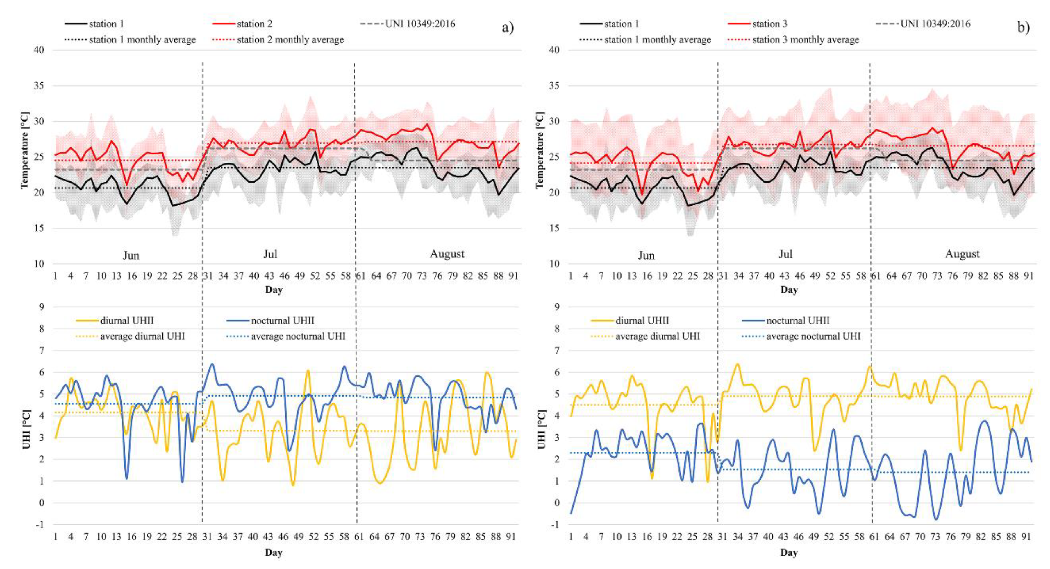
To better understand the phenomenon, the summer months (JJA) of 2018, the last full year available, were evaluated more closely, considering the average daily temperature compared with the average monthly temperature indicated by the UNI 10349: 2016 [33] standard, maximum daily temperature and diurnal and nocturnal UHII (Figure 9).
In addition to the comparison between the previously presented temperatures at stations 1, 2, and 3, Figure 9 allows us to relate these temperatures to those indicated by the UNI 10349: 2016 [33] standard. From the analysis of the graphs, it can be highlighted that the average temperatures at station 1 are generally lower than those set out in the standard in June, July, and in the second half of August; instead, they are closer to the ones of the standard in the first half of August. Indeed, for station 1, the average monthly temperatures are 2 °C to 3 °C lower than those set out in the standard. The temperatures recorded at station 2 are instead higher during all three months considered, except for some sporadic days and for the month of July. In this case, although temperatures are slightly higher, the average values are very similar to those of the UNI 10349 standard (27 °C recorded as monthly average at station 2 against 26.2 °C, monthly average temperature according to the standard). Overall, it can be observed that the average monthly temperatures of station 2 during the summer period of 2018 have been between 0.8 and 2.7 °C higher than standard. Temperatures recorded at station 3 show a similar trend than those recorded at station 2, but with a lower deviation from the standard. In August 2018 the average monthly temperature recorded at station 2 is 2 °C higher than the standard one, while the difference between real and standard temperatures is 0.9 °C for June and only 0.5 °C for July. The comparison between diurnal and nocturnal UHII at stations 2 and 3, shows significant differences. The nocturnal UHII intensity at station 2 is higher during the night (maximum of 6.4 °C and average of 4.8 °C) than the diurnal one (maximum of 6 °C and average of 3.6 °C). Both intensities show always a positive value, which means that on all the days considered, the temperatures recorded at station 2 are higher than those recorded at station 1. Conversely at station 3, nocturnal UHII (maximum of 3.7 °C and average of 1.7 °C) is generally lower than diurnal one (maximum of 6.4 °C, average of 4.8 °C). For station 3, sometimes the night temperatures are below the ones recorded at station 1 and, therefore, for 10 days the values of nocturnal UHII are negative. The month with higher differences of average diurnal and nocturnal UHII between stations 2 and 3 is August, when the diurnal UHII at station 2 is 1.6 °C lower than the one at station 3 and the nocturnal UHII at station 2 is 3.4 °C higher than the one at station 3.
3.3. Sample Year and Standard Comparison
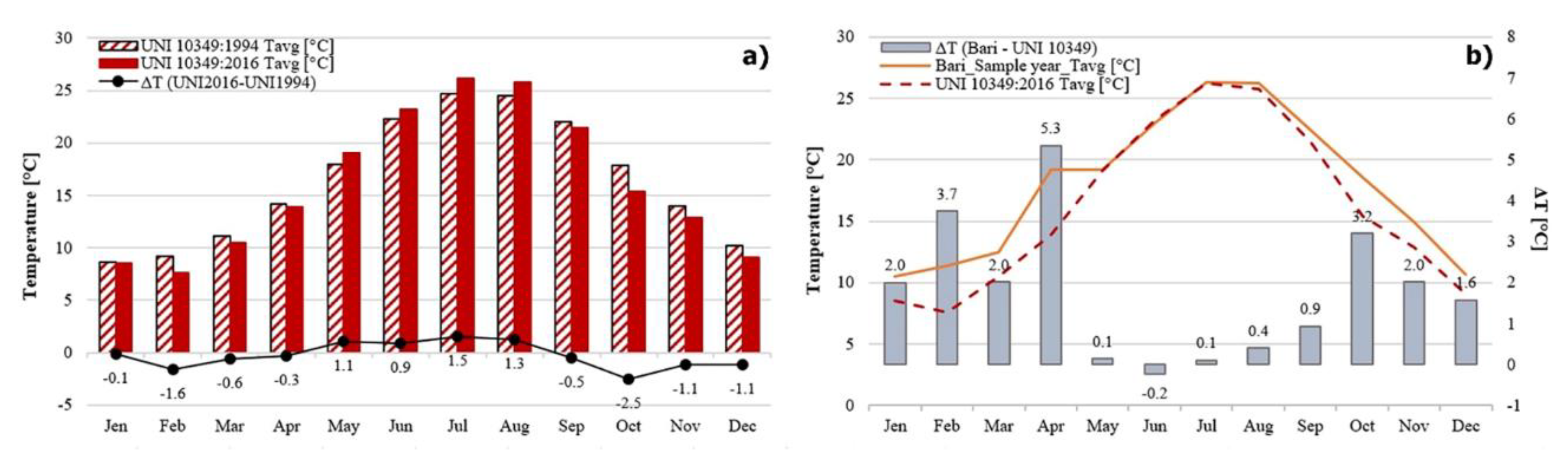
The UNI 10349-1: 2016 [33] standard provides conventional climatic data for the Italian territory, useful for verifying the energy performance of buildings. The standard includes the data of the monthly average temperatures for selected locations including the city of Bari. In this section we have compared the data from the UNI 10349: 2016 standard, the one from the previous edition of the standard, UNI 10349: 1994, dated more than 20 years before the current one, and those collected during the present study in the city of Bari via fixed weather stations. This comparison was made to assess any matches between the temperatures indicated and forecast by the standard and those recorded in the area through meteorological stations. To carry out this final comparison, a reference year was created. Since the temperatures collected derive from different meteorological stations located in different areas of the city, to obtain a reference year that could be as representative as possible of the entire city and not of only one zone, the standard year was obtained by averaging the monthly temperature values of all three stations and of all the five years considered.
Figure 10a shows that the current edition of the standard indicates lower monthly temperatures than the previous one, with the exception of the summer months, between May and August, where temperatures are around 1.0 °C higher, up to a maximum of 1.5 °C in July. Figure 10b shows the monthly temperatures referring to the sample year created and the typical one suggested by legislation. Between May and August, the temperatures are very similar to each other with differences of a few tenths of a degree; the biggest difference is found in April (5.3 °C), followed by the months of February (3.7 °C) and October (3.2 °C). Instead, the differences in the remaining months are around 2.0 °C.
3.4. Frequency Distribution of Current Temperature and Future Weather Scenarios
The final aim of the study was to predict the impact of UHI in future scenarios in order to define future threats to urban liveability. Therefore, a statistical analysis of current and future air temperature values was performed.
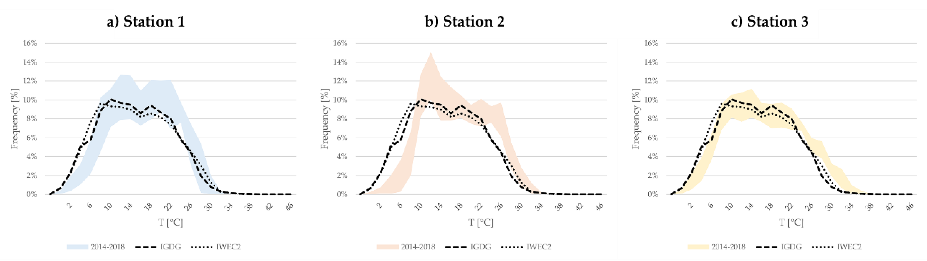
Figure 11 includes a comparison between the frequency distribution of air temperatures recorded at the four stations and the related frequency distribution of air temperatures of two typical meteorological years. The first typical year (dashed lines in the figure) is obtained from recordings taken at the Airport in the period between 1951 and 1970 and included in the Italian Climatic data collection "Gianni De Giorgio" (IGDG) [46]. The second typical year (pointed line in the figures) is obtained from recordings taken at the Airport in the period between 1984 and 2008 and included in the version 2.0 of the International Weather for Energy Calculation (IWEC2) database managed by the American Society of Heating, Refrigerating and Air-Conditioning Engineers (ASHRAE) [47]. Therefore, both files represent typical historical years. The three shadowed areas in Figure 11 represent the envelope of the frequency distributions of air temperatures recorded in the period 2014–2018 at the three weather stations. The graphs can be analysed considering three temperature ranges: cold (below 10 °C), mild (between 10 °C and 22 °C) and warm (over 22 °C).
Station 1 shows a frequency distribution of cold air temperatures with a pattern similar to the one of the two typical years but shifted of about 0 °C–2 °C towards mild temperatures. The frequency distribution of mild temperatures during the period between 2014 and 2018 is in line with the one of the two typical years. The frequency distribution of hot temperatures recorded at station 1 during the period between 2014 and 2018 shows data in line with the typical years, but with a reduced frequency of temperatures over 26 °C. This is due to the sea breeze phenomenon, particularly evident at station 1, which can counterbalance the climate change effects.
Station 2 shows a frequency distribution of cold air temperatures with a pattern similar to the one of the typical years but shifted of about 2 °C to 4 °C towards mild temperatures. Moreover, while the frequency distribution of mild temperatures is in line with the one of typical meteorological years, the frequency distribution of warm temperatures shows a shift of about 0 °C to 4 °C in comparison with the one of typical meteorological years.
Finally, station 3 shows the lower limit of the envelope of the frequency distribution of air temperatures that overlaps with the frequency distribution of air temperatures of typical meteorological years for both cold and warm temperature ranges.
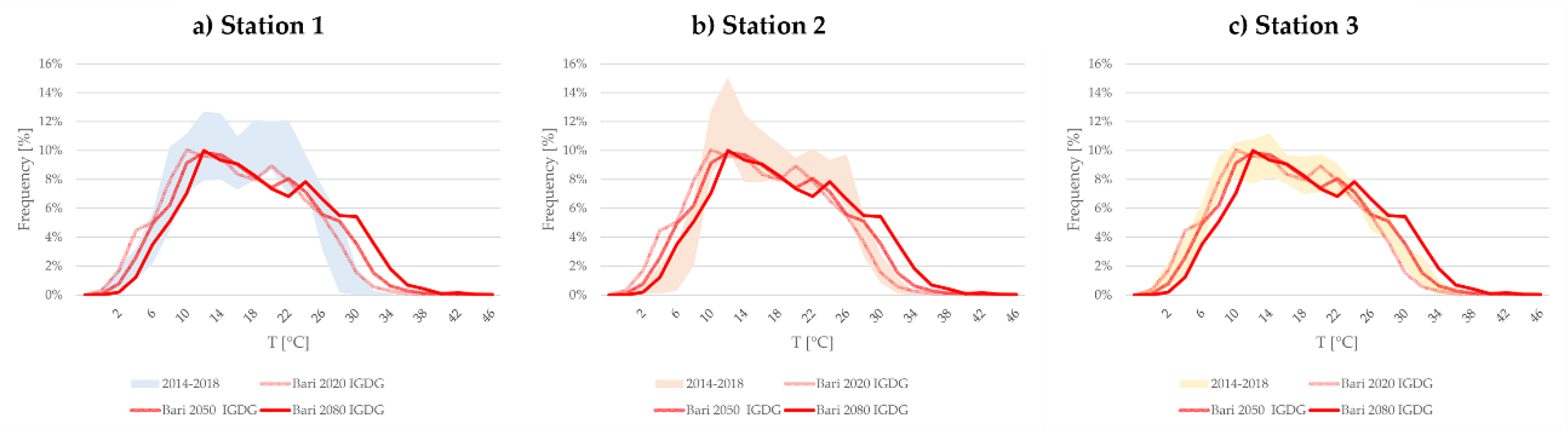
Figure 12 includes an overlap of the frequency distribution of air temperatures recorded at the three weather stations with the frequency distribution of air temperatures in future weather scenarios based on the weather files obtained from the IGDG database. The future weather scenarios have been produced using the Climate Change World Weather Generator tool developed by Jentsch et al. [48] using the statistical downscaling morphing method [49]. Furthermore, the prediction is based on the scenario A2 developed by the Intergovernmental Panel for Climate Change (IPCC) [50].
As can be observed from the graphs, the future scenario for 2020 (including the average temperatures predicted for the period 2011–2040) fits well with the current distribution of air temperatures for station 1, while it underestimates the temperatures at stations 2 and 3. It can be recognized that for both stations 2 and 3, the frequency distribution of warm air temperatures measured in the period 2014–2018 is shifted of about 0 °C–2 °C towards higher temperatures in comparison with the frequency distribution of air temperatures of the 2020 future scenario. This can be recognized as the average UHI penalty for both stations 2 and 3.
Finally, the frequency distribution of air temperatures for the scenarios of 2050 (average between 2041 and 2070) and 2080 (average between 2071 and 2100) show a further increase in average temperatures of about, respectively, 2 °C and 4 °C for the 2050 and 2080 scenarios in comparison with the 2020 one.
4. Discussion and Conclusions
Among the four selected weather stations, three of them (stations 1, 2, 3) are included in an area with a maximum distance from the coastline of less than 2 km and therefore are affected by a synergic effect of sea and land breeze, and UHI phenomenon. The fourth one (station 4) is, instead, located in a rural area far from the coastline. From the analysis of the hourly data of temperatures collected over the five years of monitoring, it is evident that station 4 shows the lowest values both in the average temperature (16.4 °C) and in the minimum one (−3.2 °C).
Nevertheless, as explained above, station 4 was excluded in the assessment of UHI intensity in Bari, since it is located too far from the coastline. For this reason, and following other studies carried out in coastal cities [44,45,51] and relevant indications from the literature [40,52], the urban weather station located in the proximity of the coastline (station 1) has been selected as the reference station.
By analysing the average monthly temperatures, we found a maximum UHIIm of 6.6 °C for both stations during the summer season (JJA period). This result is in line with what has been reported for Sydney (Australia) by Santamouris et al., who did find a maximum monthly UHII between 3.7 °C and 8.5 °C and concentrated in the summer period (November to February for Sydney).
On average, the UHIIy reaches the maximum value over the five years of 2 °C for station 2 and of 1 °C for station 3.
The maximum hourly values of UHII (UHIImax) also show a distribution very close to the one found in other studies in coastal Mediterranean cities reported in literature. In our study we did found that, depending on the season, UHIImax between 2 °C and 4 °C occur in about 40% to 50% of the days at station 2, and that during the summer season over 30% of days show UHIImax higher than 4 °C. Similar values can be found in the study of Giannaros and Melas [42]. The paper reported that in a Mediterranean coastal city (Thessaloniki, Greece), although clear seasonal variations in UHI phenomenon cannot be identified, UHI is more pronounced in the period between June and August, with maximum UHII always higher than 2 °C and sometimes approaching 3 °C.
For station 3, instead, there is a more uniform distribution of values of UHIImax. This is due to the morphology of the site, which shows a lower density and a higher percentage of greenery in comparison with the urban area monitored with station 2. Therefore, for station 3 lower values of UHIImax are recorded, with 47% to 73% of days all seasons except the summer one showing values lower than 3 °C. Moreover, this prediction is in line with the existing literature. As an example, Papanastasiou and Kittas [53] reported for a medium coastal city (Volos, Greece) an occurrence of UHIImax between 1 °C and 3 °C for over 90% of the time both in winter and in summer. It must be noted that the city of Volos is about half of the size of Bari in terms of population, but with a density of about 15% of the one in Bari and, therefore, with much lower expected values of UHII. A significant difference can be found, instead, for station 3 during summer period, when the most frequent UHIImax is between 4 °C and 5 °C (33% of days).
Finally, from the analysis of the diurnal and nocturnal variation in UHII, it can be observed the difference pattern between stations 2 and 3. The site with higher density and lower percentage of greenery (station 2) shows, during the summer period, nocturnal UHII always higher than the diurnal one, with an average monthly nocturnal UHII between 4.5 °C and 4.9 °C (daily peak of 6.4 °C) and an average monthly diurnal UHII between 3.3 °C and 4.2 °C (daily peak of 6 °C). On the contrary, the site with lower density and higher percentage of greenery (station 3) shows, during the summer period, nocturnal values of UHII much lower than the diurnal ones, with an average monthly nocturnal UHII between 1.4 °C and 2.3 °C (daily peak of 3.7 °C), and an average monthly diurnal UHI between 4.5 °C and 4.9 °C (daily peak of 6.4 °C). Moreover, while at station 2 nocturnal UHII never shows negative values, at station 3, nocturnal UHII on about 10% of days is lower than zero (i.e., station 3 records temperature values during the night-time that are lower than the ones of the reference station placed in proximity to the coastline).
Based on these data and the physical characteristics of the areas considered, some considerations can be made. The choice of weather stations resulted from the need to represent different urban contexts. The recorded and collected temperature data confirm the underlying reason for our choice and they lead to some assumptions that account for the differences in temperatures:
- (a)
- Moving away from weather station 4 to those located in Bari, by merely comparing the images of the areas, it is evident that the presence of the vegetation diminishes: weather station 4, although not being located in an isolated rural area, is surrounded by more vegetation than stations 3 and 2.
- (b)
- Another key feature for the formation of UHI is urban geometry. Geometry influences wind flows, energy absorption, and the ability of a given surface to emit long-wave radiation back to the atmosphere. In built-up areas, where the presence of obstacles prevents the quick release of heat, surfaces, and structures become large thermal masses. Unsurprisingly, urban canyons, as it is the case of station 2, play an essential role. It is thus evident that because of urban geometry, the area in which station 2 is located is the most disadvantaged one and then subject to temperature increase. In contrast, temperatures are lower at station 3, which has a less built-up area density, and even lower at weather station 4, which is the closest representation of a non-urban area.
- (c)
- Anthropogenic heat contributes to the atmospheric heat islands. Thus, in general, locations with more infrastructures, like station 2, show more anthropogenic heat than those with fewer infrastructures, like stations 1 or 4.
- (d)
- As explained above, station 1—near the sea—is affected by the sea breeze phenomenon [16]. During the heat wave of August 2018, it recorded lower temperatures than those of the other stations (reaching a maximum temperature of 28.3 °C compared to 30 °C at the others). Moreover, compared to the temperatures recorded by the other meteorological stations, the temperature peaks for station 1 are considerably lower, and the trend of maximum temperatures is more constant. In terms of sea breeze, coastal wind is generated by the differential heating of the land and the water [54,55]. When the temperature over the land is higher than the neighbouring water, the air above it is heated and rises. Then, at lower levels, the air is replaced by cooler air flowing by advection from the adjacent sea areas. Sea breezes regularly influence coastal temperatures [56]. If there is enough moisture in the atmosphere, clouds and precipitation may form. It means that the sea breeze can modify the UHI pattern, and during summer, sea breezes can reduce and delay the Heat Island circulation (HIC). This justifies the drop in temperatures recorded at weather station 1. What we did find is a common phenomenon in coastal cities. As an example, a study carried out on a small Mediterranean town (Chania, Crete) led to a similar result. It has been verified that, in this small coastal town, subjected to rapid urbanization in recent years, when moving from the coastal line to the city centre, comfort conditions become worse [22].
- (e)
- The distribution of current air temperatures at the three weather stations analysed fits well with the climate change prediction for the period 2011–2040 obtained by statistically downscaling with the IPCC A2 scenario the available data on the typical meteorological year for the period 1951–1970. A further increase of air temperature of between 2 °C to 4 °C is expected to be reached in the period 2071-2100, exacerbating the current treats to urban liveability.
In conclusion, based on this analysis of the variation in temperatures in the area of Bari and its provinces, we can reasonably assert that the phenomenon of Urban Heat Island exists; in particular, it is more pronounced in the areas closer to the city centre and gradually thins out when moving away from the city centre, with specific effects in coastal areas. This difference is seemingly attributed to a number of factors, like the presence/absence of vegetation, urban geometry and, in general, to the level of urbanization that also inevitably causes a different production of anthropogenic heat, all of which actively contribute to the formation of UHI.
From the data collected, both in the first phase of our study concerning the distribution of temperatures across the territory, and the subsequent detailed analysis of the UHI intensity, it has been shown that the busiest and most urbanized areas tend to register higher temperatures, such as the areas where stations 2 and 3 are located. Indeed, if the two weather stations used may be deemed to be representative of the urban and rural areas, the area most exposed to this phenomenon is the one coinciding with the city centre: its geometric, environmental, climatic, and geographical characteristics are such that temperatures tend to remain higher during the day.
Finally, it has also been shown that the sea breeze phenomenon, particularly visible in the coastal area represented by the reference station (station 1), can mitigate temperatures and change the configuration of the phenomenon.
Author Contributions
Conceptualization, A.M., D.-D.K. and F.F.; methodology, A.M., D.-D.K. and F.F.; validation, A.M., D.-D.K. and F.F.; formal analysis, A.M. and F.F.; investigation, A.M.; writing—original draft preparation, A.M. and F.F.; writing—review and editing, D.-D.K.; supervision, F.F. and D.-D.K. All authors have read and agreed to the published version of the manuscript.
Funding
This research received no external funding.
Acknowledgments
The authors would like to acknowledge the Regional Environmental Protection Agency of Puglia (ARPA Puglia) and the Mediterranean Agronomic Institute (CIHEAM) for providing them with the environmental data required for the study.
Conflicts of Interest
The authors declare no conflict of interest.
References
- Grimmond, C.S.B.; Ward, H.C.; Kotthaus, S. Effects of Urbanization on local and regional climate. In The Routledge Handbook of Urbanization and Global Environmental Change; Seto, K.C., Solecki, W.D., Griffith, C.A., Eds.; Routledge: London, UK, 2015. [Google Scholar] [CrossRef]
- Boufidou, E.; Commandeur, T.J.F.; Nedkov, S.B.; Zlatanova, S. Mesure the climate, model the city. Int. Arch. Photogramm. Remote Sens. Spatial Inf. Sci. 2011, XXXVIII-4/C21, 59–66. [Google Scholar] [CrossRef] [Green Version]
- Santamouris, M.; Cartalis, C.; Synnefa, A.; Kolokotsa, D. On the impact of urban heat island and global warming on the power demand and electricity consumption of buildings—A review. Energy Build. 2015, 98, 119–124. [Google Scholar] [CrossRef]
- Santamouris, M. On the energy impact of urban heat island and global warming on buildings. Energy Build. 2014, 82, 100–113. [Google Scholar] [CrossRef]
- Santamouris, M.; Papanikolaou, N.; Livada, I.; Koronakis, I.; Georgakis, C.; Argiriou, A.; Assimakopoulos, D.N. On the impact of urban climate on the energy consuption of building. Sol. Energy 2001, 70, 201–216. [Google Scholar] [CrossRef]
- Santamouris, M. Innovating to zero the building sector in Europe: Minimising the energy consumption, eradication of the energy poverty and mitigating the local climate change. Sol. Energy 2016, 128, 61–94. [Google Scholar] [CrossRef]
- Sanchez-Guevara, C.; Núñez Peiró, M.; Taylor, J.; Mavrogianni, A.; Neila González, J. Assessing population vulnerability towards summer energy poverty: Case studies of Madrid and London. Energy Build. 2019, 190, 132–143. [Google Scholar] [CrossRef] [Green Version]
- Santamouris, M. Recent progress on urban overheating and heat island research. integrated assessment of the energy, environmental, vulnerability and health impact synergies with the global climate change. Energy Build. 2019, 109482. [Google Scholar] [CrossRef]
- Hajat, S.; Armstrong, B.; Baccini, M.; Biggeri, A.; Bisanti, L.; Russo, A.; Paldy, A.; Menne, B.; Kosatsky, T. Impact of high temperatures on mortality: Is there an added heat wave effect? Epidemiology 2006, 17, 632–638. [Google Scholar] [CrossRef] [PubMed]
- Baccini, M.; Biggeri, A.; Accetta, G.; Kosatsky, T.; Katsouyanni, K.; Analitis, A.; Anderson, H.R.; Bisanti, L.; D′Iippoliti, D.; Danova, J.; et al. Heat effects on mortality in 15 European cities. Epidemiology 2008, 19, 711–719. [Google Scholar] [CrossRef] [PubMed]
- Oke, T.R. Canyon geometry and the nocturnal urban heat island: Comparison of scale model and field observations. J. Climatol. 1981, 1, 237–254. [Google Scholar] [CrossRef]
- Oke, T.R. The energetic basis of the urban heat island. Q. J. R. Meteorol. Soc. 1982, 108, 1–24. [Google Scholar] [CrossRef]
- Doulos, L.; Santamouris, M.; Livada, I. Passive cooling of outdoor urban spaces. The role of materials. Sol. Energy 2004, 77, 231–249. [Google Scholar] [CrossRef]
- Rizwan, A.M.; Dennis, L.Y.C.; Liu, C. A review on the generation, determination and mitigation of Urban Heat Island. J. Environ. Sci. 2008, 20, 120–128. [Google Scholar] [CrossRef]
- Taha, H. Urban climates and heat islands: Albedo, evapotranspiration, and anthropogenic heat. Energy Build. 1997, 25, 99–103. [Google Scholar] [CrossRef] [Green Version]
- Vardoulakis, E.; Karamanis, D.; Fotiadi, A.; Mihalakakou, G. The urban heat island effect in a small Mediterranean city of high summer temperatures and cooling energy demands. Sol. Energy 2013, 94, 128–144. [Google Scholar] [CrossRef]
- U.S. Environmental Protection Agency. Reducing Urban Heat Islands: Compendium of Strategies. Draft. 2008. Available online: https://www.epa.gov/heat-islands/heat-island-compendium (accessed on 21 April 2020).
- Zhou, X.; Okaze, T.; Ren, C.; Cai, M.; Ishida, Y.; Watanabe, H.; Mochida, A. Evaluation of urban heat islands using local climate zones and the influence of sea-land breeze. Sustain. Cities Soc. 2020, 55. [Google Scholar] [CrossRef]
- Bauer, T.J. Interaction of urban heat island effects and land–sea breezes during a new york city heat event. J. Appl. Meteorol. Climatol. 2020, 59, 477–495. [Google Scholar] [CrossRef]
- Papanastasiou, D.K.; Melas, D.; Bartzanas, T.; Kittas, C. Temperature, comfort and pollution levels during heat waves and the role of sea breeze. Int. J. Biometeorol. 2010, 54, 307–317. [Google Scholar] [CrossRef]
- Freitas, E.D.; Rozoff, C.M.; Cotton, W.R.; Silva Dias, P.L. Interactions of an urban heat island and sea-breeze circulations during winter over the metropolitan area of São Paulo, Brazil. Bound.-Layer Meteorol. 2007, 122, 43–65. [Google Scholar] [CrossRef]
- Kolokotsa, D.; Psomas, A.; Karapidakis, E. Urban heat island in southern Europe: The case study of Hania, Crete. Sol. Energy 2009, 83, 1871–1883. [Google Scholar] [CrossRef]
- Salvati, A.; Coch Roura, H.; Cecere, C. Assessing the urban heat island and its energy impact on residential buildings in Mediterranean climate: Barcelona case study. Energy Build. 2017, 146, 38–54. [Google Scholar] [CrossRef] [Green Version]
- Geletič, J.; Lehnert, M.; Savić, S.; Milošević, D. Inter-/intra-zonal seasonal variability of the surface urban heat island based on local climate zones in three central European cities. Build. Environ. 2019, 156, 21–32. [Google Scholar] [CrossRef]
- Sailor, D.J.; Fan, H. Modeling the diurnal variability of effective albedo for cities. Atmos. Environ. 2002, 36, 713–725. [Google Scholar] [CrossRef]
- Salvati, A.; Monti, P.; Coch Roura, H.; Cecere, C. Climatic performance of urban textures: Analysis tools for a Mediterranean urban context. Energy Build. 2019, 185, 162–179. [Google Scholar] [CrossRef]
- Paramita, B.; Matzarakis, A. Urban morphology aspects on microclimate in a hot and humid climate. Geogr. Pannonica 2019, 23, 398–410. [Google Scholar] [CrossRef] [Green Version]
- Voogt, J.A. Urban Heat Island. In Encyclopedia of Global Environmental Change; Munn, T., Ed.; Wiley: Chichester, UK, 2002; Volume 3, pp. 660–666. [Google Scholar]
- Offerle, B.; Grimmond, C.S.B.; Fortuniak, K.; Kłysik, K.; Oke, T.R. Temporal variations in heat fluxes over a central European city centre. Theor. Appl. Climatol. 2006, 84, 103–115. [Google Scholar] [CrossRef]
- Hinkel, K.M.; Nelson, F.E. Anthropogenic heat island at Barrow, Alaska, during winter: 2001–2005. J. Geophys. Res. Atmos. 2007, 112. [Google Scholar] [CrossRef]
- Oke, T.R. Street design and urban canopy layer climate. Build. Environ. 1988, 11, 103–113. [Google Scholar] [CrossRef]
- Oke, T.R. The distinction between canopy and boundary-layer urban heat Islands. Atmosphere 1976, 14, 268–277. [Google Scholar] [CrossRef] [Green Version]
- UNI. 10349-1: 2016. Riscaldamento e Raffrescamento Degli Edifici—Dati Climatici. Parte 1: Medie Mensili per la Valutazione Della Prestazione Termo-Energetica Dell'edificio e Metodi per Ripartire L'irradianza Solare Nella Frazione Diretta e Diffusa e per Calcolare L'irradianza Solare su di una Superficie Inclinata. 2016. Available online: https://nt24.it/2016/02/riscaldamento-e-raffrescamento-degli-edifici-dati-climatici-in-inchiesta-pubblica/ (accessed on 21 April 2020).
- Italian National Institute of Statistics. Statistical Data. Available online: https://www.istat.it/ (accessed on 6 April 2020).
- World Meteorological Organization. Available online: https://worldweather.wmo.int/en/home.html (accessed on 29 May 2020).
- ARPA Puglia. Official Website. Available online: www.arpa.puglia.it (accessed on 21 April 2020).
- CIHEAM. Official Website. Available online: https://www.iamb.it (accessed on 21 April 2020).
- Stewart, I.D.; Oke, T.R. Local climate zones for urban temperature studies. Bull. Am. Meteorol. Soc. 2012, 93, 1879–1900. [Google Scholar] [CrossRef]
- Giridharan, R.; Kolokotroni, M. Urban heat island characteristics in London during winter. Sol. Energy 2009, 83, 1668–1682. [Google Scholar] [CrossRef]
- Sakakibara, Y.; Owa, K. Urban–Rural temperature differences in coastal cities: Influence of rural sites. Int. J. Climatol. 2005, 25, 811–820. [Google Scholar] [CrossRef]
- Acero, J.A.; Arrizabalaga, J.; Kupski, S.; Katzschner, L. Urban heat island in a coastal urban area in northern Spain. Theor. Appl. Climatol. 2013, 113, 137–154. [Google Scholar] [CrossRef]
- Giannaros, T.M.; Melas, D. Study of the urban heat island in a coastal Mediterranean City: The case study of Thessaloniki, Greece. Atmos. Res. 2012, 118, 103–120. [Google Scholar] [CrossRef]
- Anjos, M.; Lopes, A. Urban Heat Island and Park Cool Island intensities in the coastal city of Aracaju, North-Eastern Brazil. Sustainability 2017, 9, 1379. [Google Scholar] [CrossRef] [Green Version]
- Santamouris, M.; Haddad, S.; Fiorito, F.; Osmond, P.; Ding, L.; Prasad, D.; Zhai, X.; Wang, R. Urban heat island and overheating characteristics in Sydney, Australia. An analysis of multiyear measurements. Sustainability 2017, 9, 712. [Google Scholar] [CrossRef]
- Yun, G.Y.; Ngarambe, J.; Duhirwe, P.N.; Ulpiani, G.; Paolini, R.; Haddad, S.; Vasilakopoulou, K.; Santamouris, M. Predicting the magnitude and the characteristics of the urban heat island in coastal cities in the proximity of desert landforms. The case of Sydney. Sci. Total Environ. 2020, 709. [Google Scholar] [CrossRef] [PubMed]
- Weather Data Sources. Available online: https://energyplus.net/weather/sources (accessed on 5 June 2020).
- ASHRAE. International Weather for Energy Calculations 2.0 (IWEC Weather Files) DVD. 2012. Available online: https://www.ashrae.org/technical-resources/bookstore/ashrae-international-weather-files-for-energy-calculations-2-0-iwec2 (accessed on 21 April 2020).
- Jentsch, M.F.; James, P.A.B.; Bourikas, L.; Bahaj, A.S. Transforming existing weather data for worldwide locations to enable energy and building performance simulation under future climates. Renew Energy 2013, 55, 514–524. [Google Scholar] [CrossRef]
- Belcher, S.E.; Hacker, J.N.; Powell, D.S. Constructing design weather data for future climates. Build. Serv. Eng. Res. Technol. 2005, 26, 49–61. [Google Scholar] [CrossRef]
- IPCC. Climate Change 2014: Syntesis Report. In Contribution of Working Groups I, II and III to the Fifth Assessment Report of the Intergovernmental Panel on Climate Change; IPCC: Geneva, Switzerland, 2014; p. 151. [Google Scholar]
- Livada, I.; Synnefa, A.; Haddad, S.; Paolini, R.; Garshasbi, S.; Ulpiani, G.; Fiorito, F.; Vassilakopoulou, K.; Osmond, P.; Santamouris, M. Time series analysis of ambient air-temperature during the period 1970–2016 over Sydney, Australia. Sci. Total Environ. 2019, 648, 1627–1638. [Google Scholar] [CrossRef]
- Oke, T.R. Initial Guidance to Obtain Representative Meteorological Observations at Urban Sites; Report prepared for the World Meteorological Organization, Instruments and observing methods, Report no. 81; World Meteorological Organization (WMO): Geneva, Switzerland, 2004. [Google Scholar]
- Papanastasiou, D.K.; Kittas, C. Maximum urban heat island intensity in a medium-sized coastal Mediterranean city. Theor. Appl. Climatol. 2012, 107, 407–416. [Google Scholar] [CrossRef]
- Estoque, M.A. A theoretical investigation of the sea breeze. Q. J. R. Meteorol. Soc. 1961, 87, 136–146. [Google Scholar] [CrossRef]
- Rotunno, R. On the linear theory of the land and sea breeze. J. Atmos. Sci. 1983, 40, 1999–2009. [Google Scholar] [CrossRef]
- Simpson, J.E.; Mansfield, D.A.; Milford, J.R. Inland penetration of sea-breeze fronts. Q. J. R. Meteorol. Soc. 1977, 103, 47–76. [Google Scholar] [CrossRef]
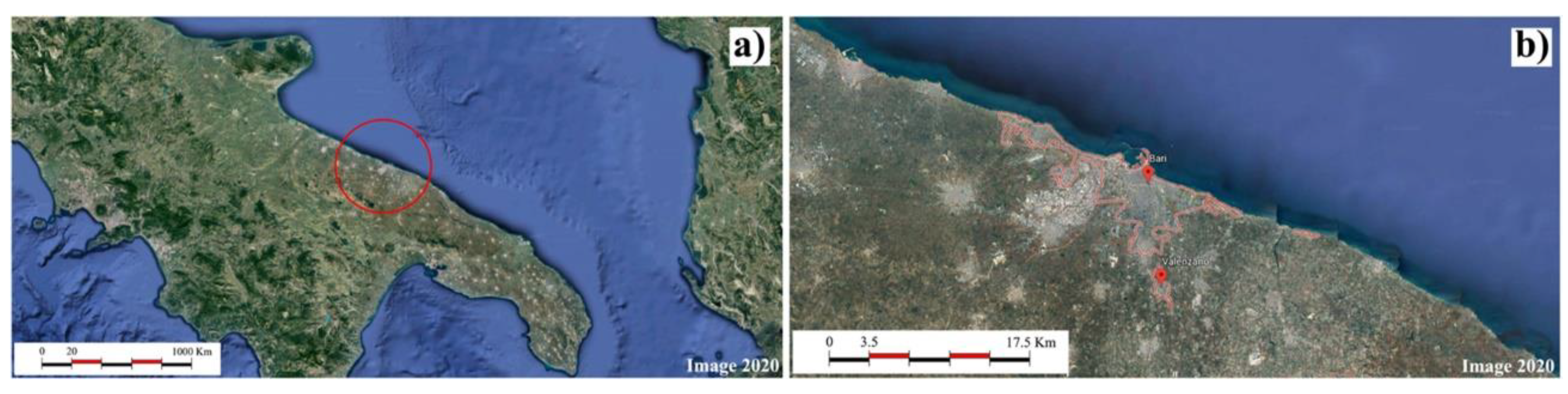
Figure 1.
Google Earth image of (a) geographic location of Bari and (b) Bari and Valenzano areas.

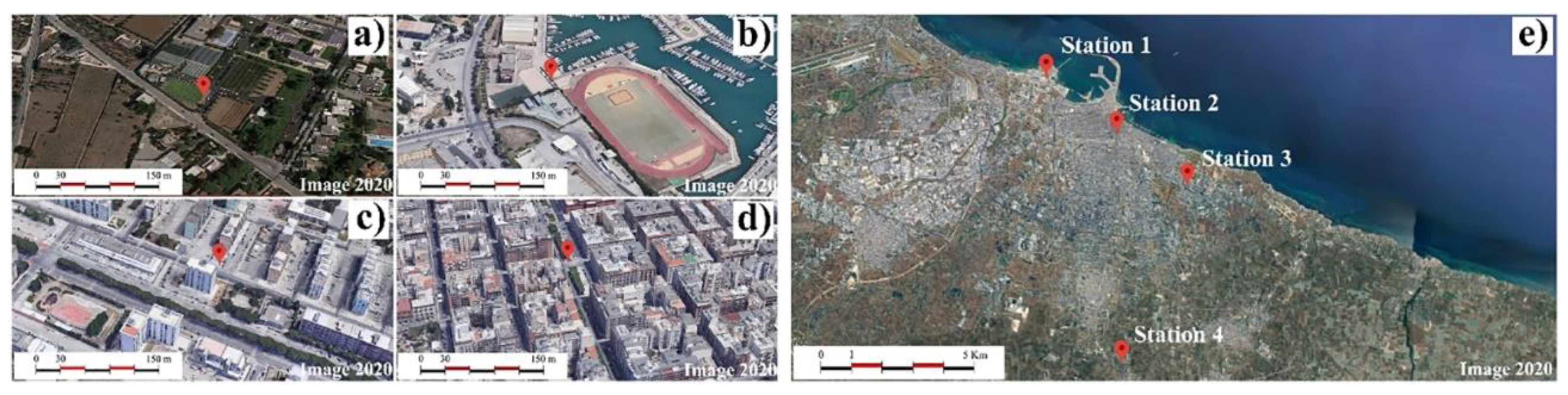
Figure 2.
(a) Station 4 area, (b) station 1 area; (c) station 3 area; (d) station 2 area; (e) locations of the weather stations.
Figure 2.
(a) Station 4 area, (b) station 1 area; (c) station 3 area; (d) station 2 area; (e) locations of the weather stations.

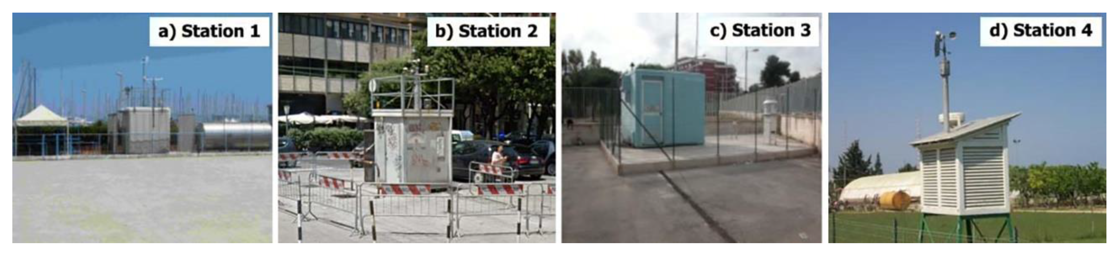
Figure 3.
View from the ground of the four weather stations: (a) weather station 1 positioned near the University Sport Centre, (b) weather station 2 at corso Cavour, (c) weather station 3 at via Caldarola, (d) weather station 4 at the Mediterranean Agronomic Institute in Valenzano.
Figure 3.
View from the ground of the four weather stations: (a) weather station 1 positioned near the University Sport Centre, (b) weather station 2 at corso Cavour, (c) weather station 3 at via Caldarola, (d) weather station 4 at the Mediterranean Agronomic Institute in Valenzano.

Figure 4.
Statistical analysis of hourly temperatures at the four stations: maximum value, minimum value, first quartile, average, third quartile.
Figure 4.
Statistical analysis of hourly temperatures at the four stations: maximum value, minimum value, first quartile, average, third quartile.

Figure 5.
Hourly data of air temperature in August and December from 2014 to 2018. Blue hourly air temperature values for station 1, orange hourly air temperature values for station 2, yellow hourly air temperature values for station 3, green hourly air temperature values for station 4.
Figure 5.
Hourly data of air temperature in August and December from 2014 to 2018. Blue hourly air temperature values for station 1, orange hourly air temperature values for station 2, yellow hourly air temperature values for station 3, green hourly air temperature values for station 4.

Figure 6.
Monthly average temperatures, monthly maximum and minimum temperatures from 2014 to 2018.

Figure 7.
Seasonal distribution of daily values of maximum hourly difference of temperature recorded during each day (UHIImax) at (a) stations 2 and (b) 3.
Figure 7.
Seasonal distribution of daily values of maximum hourly difference of temperature recorded during each day (UHIImax) at (a) stations 2 and (b) 3.

Figure 8.
Diurnal and nocturnal UHII from 2014 to 2018, recorded at (a) station 2, and (b) station 3.
Figure 8.
Diurnal and nocturnal UHII from 2014 to 2018, recorded at (a) station 2, and (b) station 3.

Figure 9.
(a) Diurnal and nocturnal UHII at station 2 and comparison between stations 1 and 2 during June, July, and August; (b) diurnal and nocturnal UHII at station 3 and comparison between stations 1 and 3 during June, July, and August.
Figure 9.
(a) Diurnal and nocturnal UHII at station 2 and comparison between stations 1 and 2 during June, July, and August; (b) diurnal and nocturnal UHII at station 3 and comparison between stations 1 and 3 during June, July, and August.

Figure 10.
(a) Comparison between UNI 10349:1994 and UNI 10349:2016 temperature data; (b) Comparison between the sample year and UNI 10349: 2016 temperature data.
Figure 10.
(a) Comparison between UNI 10349:1994 and UNI 10349:2016 temperature data; (b) Comparison between the sample year and UNI 10349: 2016 temperature data.

Figure 11.
Frequency distribution of air temperature values recorded at stations 1, 2, and 3 and comparison with the frequency distribution of air temperatures of typical meteorological years from IGDG (1951–1970) and IWEC2 (1984–2008) databases: (a) frequency distribution of air temperatures at station 1, (b) frequency distribution of air temperatures at station 2, (c) frequency distribution of air temperatures at station 3.

Figure 12.
Frequency distribution of air temperature values recorded at station 1, 2, and 3 and comparison with the frequency distribution of air temperatures of future weather scenarios: (a) frequency distribution of air temperatures at station 1, (b) frequency distribution of air temperatures at station 2, (c) frequency distribution of air temperatures at station 3.


Table 1.
Classification of the Local Climatic Zone (LCZ) for each station. In parentheses are limits for each parameter according to Stewart and Oke (2012) [38].
Table 1.
Classification of the Local Climatic Zone (LCZ) for each station. In parentheses are limits for each parameter according to Stewart and Oke (2012) [38].
| Station nr. | Local Climate Zone | Built Type | Sky-View Factor | Aspect Ratio | Building Surface Fraction | Height of Roughness Elements |
|---|---|---|---|---|---|---|
| 1 | LCZ 9G | Sparsely built with water | 0.85 (>0.8) | 0.28 (0.1–0.25) | 12 (10–20) | 8 (3–10) |
| 2 | LCZ 2 | Compact mid-rise | 0.45 (0.3–0.6) | 1.25 (0.75–2) | 50 (40–70) | 25 (10–25) |
| 3 | LCZ 5 | Open mid-rise | 0.65 (0.5–0.8) | 0.75 (0.3–0.75) | 32 (20–40) | 15 (10–25) |
| 4 | LCZ 9B | Sparsely built with scattered trees | 0.9 (>0.8) | 0.16 (0.1–0.25) | 19 (10–20) | 6 (3–8) |
Table 2.
Percentage of missing data for each station from 2014 to 2018.
| % of Missing Data | |||||
|---|---|---|---|---|---|
| 2014 | 2015 | 2016 | 2017 | 2018 | |
| Station 1 | 2.8% | 2.1% | 5.8% | 10.1% | 0.4% |
| Station 2 | 0.0% | 2.0% | 0.0% | 0.0% | 0.0% |
| Station 3 | 2.2% | 2.6% | 1.6% | 0.0% | 1.7% |
| Station 4 | 0.0% | 0.0% | 0.0% | 0.0% | 0.0% |
Table 3.
Values of Urban Heat Island Intensity (UHII) monthly average temperatures (UHIIm) and annual average temperature (UHIIy) at stations 2 and 3.
Table 3.
Values of Urban Heat Island Intensity (UHII) monthly average temperatures (UHIIm) and annual average temperature (UHIIy) at stations 2 and 3.
| UHIIm [°C] | UHIIy | |||||||||||||
|---|---|---|---|---|---|---|---|---|---|---|---|---|---|---|
| Station | Year | Jan | Feb | Mar | Apr | May | Jun | Jul | Aug | Sep | Oct | Nov | Dec | [°C] |
| 2 | 2014 | 1.2 | 1.0 | 1.4 | 0.8 | 0.8 | 0.7 | 0.7 | 1.0 | 0.8 | 0.8 | 0.7 | 1.5 | 1.0 |
| 2015 | 0.8 | 1.9 | 2.4 | 1.3 | 1.3 | 4.1 | 1.1 | 1.0 | 1.2 | 0.9 | 1.2 | 1.2 | 1.6 | |
| 2016 | 1.2 | 1.1 | 1.0 | 1.0 | 1.0 | 1.0 | 1.0 | 0.7 | 0.7 | −0.3 | −2.3 | −0.1 | 0.5 | |
| 2017 | - | −2.1 | −1.5 | −1 | −1 | 4.3 | 1.8 | 2.5 | 2.5 | 2.2 | 2.1 | 2.3 | 1.1 | |
| 2018 | 2.3 | 1.9 | 2.8 | 3.2 | 3.2 | 6.6 | 3.5 | 3.7 | 0.8 | −0.5 | −1.6 | −1.7 | 2.0 | |
| 3 | 2014 | −0.2 | 0 | 0.5 | 0.8 | 0.8 | 0.9 | 0.8 | 1.0 | 0.6 | 0.1 | −0.2 | −0.2 | 0.4 |
| 2015 | 0.0 | 0.8 | 1.4 | 0.7 | 0.7 | 4.1 | 1.4 | 0.8 | 0.6 | −0.1 | 0.0 | −0.1 | 0.9 | |
| 2016 | −0.1 | −0.1 | 0.1 | 0.5 | 0.5 | 0.9 | 1.1 | 0.5 | −0.2 | −1.6 | −3.7 | −1.5 | −0.3 | |
| 2017 | - | −3.5 | −2.6 | −1.7 | −1.7 | 4 | 1.5 | 2 | 1.4 | 1 | 0.3 | 0.5 | 0.1 | |
| 2018 | 0.5 | 0.4 | 1.3 | 2.6 | 2.6 | 6.6 | 3.2 | 3.1 | 0.0 | −1.8 | −3.1 | −3.3 | 1.0 | |
Table 4.
Maximum average daily temperatures (UHIId) for stations 2 and 3.
| Year | Date | Reference [°C] | Station [°C] | UHIId [°C] | |
|---|---|---|---|---|---|
| Station 2 | 2014 | 23/12 | 8.5 | 12.9 | 4.4 |
| 2015 | 19/5 | 18.8 | 23.5 | 4.7 | |
| 2016 | 13/7 | 28.4 | 30.9 | 2.5 | |
| 2017 | 21/11 | 8.0 | 11.4 | 3.4 | |
| 2018 | 28/3 | 6.5 | 12.0 | 5.5 | |
| Station 3 | 2014 | 23/05 | 20.4 | 22.4 | 2.0 |
| 2015 | 19/5 | 18.8 | 23.0 | 4.2 | |
| 2016 | 13/7 | 28.4 | 31.2 | 2.8 | |
| 2017 | 10/8 | 29.4 | 32.4 | 3.0 | |
| 2018 | 02/7 | 23.2 | 27.9 | 4.6 |
© 2020 by the authors. Licensee MDPI, Basel, Switzerland. This article is an open access article distributed under the terms and conditions of the Creative Commons Attribution (CC BY) license (http://creativecommons.org/licenses/by/4.0/).
Share and Cite
MDPI and ACS Style
Martinelli, A.; Kolokotsa, D.-D.; Fiorito, F. Urban Heat Island in Mediterranean Coastal Cities: The Case of Bari (Italy). Climate 2020, 8, 79. https://0-doi-org.brum.beds.ac.uk/10.3390/cli8060079
AMA Style
Martinelli A, Kolokotsa D-D, Fiorito F. Urban Heat Island in Mediterranean Coastal Cities: The Case of Bari (Italy). Climate. 2020; 8(6):79. https://0-doi-org.brum.beds.ac.uk/10.3390/cli8060079
Chicago/Turabian StyleMartinelli, Alessandra, Dionysia-Denia Kolokotsa, and Francesco Fiorito. 2020. "Urban Heat Island in Mediterranean Coastal Cities: The Case of Bari (Italy)" Climate 8, no. 6: 79. https://0-doi-org.brum.beds.ac.uk/10.3390/cli8060079
Note that from the first issue of 2016, this journal uses article numbers instead of page numbers. See further details here.