Long-Term Rainfall Trends and Their Variability in Mainland Portugal in the Last 106 Years


1
Instituto Superior Técnico (IST), Civil Engineering Research and Innovation for Sustainability (CERIS), 1040-001 Lisbon, Portugal
2
National Laboratory for Civil Engineering (LNEC), 1700-075 Lisbon, Portugal
3
Faculty of Civil Engineering, Institute of Environmental Engineering, Technical University of Košice, 042 00 Košice, Slovakia
*
Author to whom correspondence should be addressed.
†
Current address: Department of Civil Engineering, Architecture and Georesources (DECivil), Instituto Superior Tecnico (IST), The University of Lisbon (Universidade de Lisboa), Av. Rovisco Pais, No. 1, 1040-001 Lisbon, Portugal.
Climate 2020, 8(12), 146; https://0-doi-org.brum.beds.ac.uk/10.3390/cli8120146
Submission received: 13 November 2020
/
Revised: 3 December 2020
/
Accepted: 7 December 2020
/
Published: 10 December 2020
(This article belongs to the Special Issue Climate Variability and Drought Management)
Abstract
:This study addresses the long-term rainfall trends, their temporal variability and uncertainty over mainland Portugal, a small country on the most western European coast. The study was based on monthly, seasonal and annual rainfall series spanning for a period of 106 years, between October 1913 and September 2019 (herein after referred to as global period), at 532 rain gauges evenly distributed over the country (c.a. 6 rain gauges per 1000 km). To understand the rainfall behavior over time, an initial sub-period with 55 years and a final sub-period with 51 years were also analyzed along with the global period. The trends identification and the assessment of their magnitude were derived using the nonparametric Mann-Kendall (MK) test coupled with the Sen’s slope estimator method. The results showed that after the initial sub-period with prevailing increasing rainfall, the trends were almost exclusively decreasing. They were also so pronounced that they counterbalanced the initial rainfall increase and resulted in equally decreasing trends for the global period. The study also shows that approximately from the late 1960s on, the rainy season pattern has changed, with the last months prior to the dry season showing a sustained decrease of their relative contributions to the annual rainfalls. Overall, the results support the hypothesis of less uncertainty on the pronounced decrease of rainfall over mainland Portugal in recent years, which is expected to continue. They also show that the asymmetry between a less wet North, yet still wet, and an arid South is becoming much more marked.
1. Introduction
Progressively more noticeable signs of climate change have been detected in recent years, in the form of increased climate variability, more and worse extreme hydrological events, rising temperature and sea level, among others [1,2,3]. Such signs have become large enough to exceed the bounds of their historical natural variability.
According to the periodical reports of the Intergovernmental Panel on Climate Change, IPCC [4,5,6], the increasing sea surface temperature and the consequent intensification of the hydrological cycle [7] has a significant effect on the rainfall, which is expected to increase globally [8]. Nevertheless, at regional and local scales, decreasing trends in rainfall are also expected [4,9]. This is the case of the Iberian Peninsula, in which mainland Portugal is located, where the rainfall amounts are projected to decrease throughout the 21st century, and become more clustered into extreme rainfall events [10,11,12,13,14,15].
Regarding the recent climate evolution, the high northern latitudes have registered rainfall increases, while from 10 S to 30 N decreases were reported from the 1970s onward [7]. This also applies to Europe, with increasing rainfall in its higher latitudes and decreasing rainfall in the Mediterranean region particularly in its western and central parts [16]. Such decrease in the rainfall is aligned with the general trend throughout the 21st century pointed out by Gibelin and Déqué [17] and Giorgi and Lionello [18].
Specifically for the Mediterranean region, there are several studies making use of ground-based data about rainfall, drought characteristics, and moisture availability trends during the 20th century, e.g., [19,20,21,22,23], but few have addressed climate variability in the early years of the 21st century, e.g., [24,25,26]. However, such type of studies needs to be continuously updated, as the changes of most of the hydrological variables are related to active and ongoing processes that may be more or less visible depending on the materials and models, time-windows, and lengths of the analyzed time series data.
Rainfall is the source of water of the hydrological cycle [9,27]. Hence, the detection and quantification of trends and of abrupt changes (within-the-year or among years) in its series are fundamental issues to understand the susceptibility of the hydrological environment to the effects of the climate change, namely in terms of freshwater availability. With this in mind, long-term and recent rainfall trends at different time scales, and their fluctuation and uncertainty are analyzed for mainland Portugal aiming at understanding how they changed over time.
A decrease in the rainfall has been generally pointed out for mainland Portugal. However, the results from the general circulation models (GCM) applied to different climate scenarios show substantial differences, meaning that there is a considerable uncertainty about future projections of the rainfall amounts and that the numerical models of climate change prediction are in need for further insights [14,15]. To reduce uncertainty in rainfall changes studies, the use of spatially dense ground-based observations can be an alternative to the GCM. For this purpose, long data series must be available at a high number of monitoring points to ensure a comprehensive description of the temporal and spatial variability of the rainfall at different timescales over the study region [28,29].
However, most of the studies on the topic for Portugal have been based on a few rain gauges or on rainfall series generally with short records length. This was the case of the novel studies of Portela and Carvalho Quintela [30,31], which used monthly rainfall series, almost from the beginning to the end of the 20th century (average length of the records of 90 years), but only at 11 rain gauges scattered over the country. Following the previous studies, it is worth mentioning de Lima et al. [32], which used 107 rain gauges with 69 years of monthly data, from 1941 to 2000; Rodrigo and Trigo [33], which addressed rainfall trends over the Iberian Peninsula, from 1951 to 2002, based on 22 rain gauges, 7 of which located in Portugal; and the wide-ranging analysis of Santos and Portela [34], which used 94 years, from 1910 to 2004, of monthly rainfall series at 144 rain gauges regularly distributed over the country. The last authors showed that the high spatial rainfall variability hampers the establishment of an overall pattern of the rainfall changes. In fact, most of the detected monthly and annual rainfall trends had no statistical significance (except for March with generalized pronounced decrease), but instead were within the limits of the natural temporal rainfall variability.
Other contributions on the subject for mainland Portugal using ground-based observations are those of de Lima et al. [35,36], based on only 10 rain gauges over Portugal, albeit with long recording series, and of Santo et al. [16], and de Lima et al. [37] that used daily data from 1941 to 2007 at 57 rain gauges to ascertain seasonal variations and trends in the intensity, frequency and duration of daily rainfall extremes. Portela et al. [38] summarizes previous studies done by the authors to Portugal, including trend analysis applied to streamflow series, and Nunes and Lourenço [39] analyzes the monthly and annual rainfall trends from 1960 to 2011 at 42 rain gauges. A more recent study by Portela et al. [26] used 108 years of monthly records at 62 rain gauges densely covering part of southern Portugal (study area of 16,000 km, i.e., approx. 18% of mainland Portugal) where the rainfall decrease is a major problem due to the water scarcity that already characterizes the region [40]. Such study revealed that in general, the upward rainfall trends in the early years of the 20th century switched to pronounced significant downward trends in recent years. It also revealed that the intra-annual rainfall pattern is changing, namely in what concerns the more contributory months of the year.
The present research work updates the results from the previous studies, with emphasis on those of Portela et al. [26] by expanding them to the entire country, employing up-to-date ground-based data covering both a long period (106 years, from 1913/1914 to 2018/2019) and a large number of rain gauges (532 rain gauges, c.a., 6 rain gauges per 1000 km) thus, providing a comprehensive assessment of the temporal and spatial rainfall variability over Portugal.
Following this introduction, Section 2 presents the study area, the rainfall data that supported the research, the procedure applied to fill in the monthly rainfall gaps, and the models used to characterize the rainfall trends. Section 3 reports the results achieved. Finally, Section 4 provides a discussion and some relevant conclusions from the trend analysis.
The main findings of this research evidence a widespread decrease of the rainfall over Portugal, especially from 1960 onwards, that is also resulting in a more pronounced asymmetry between a still relatively wet North and a dry South. The overall rainfall decrease is becoming less uncertain, reinforcing the evidence of a future with less freshwater availability and, consequently, the need for widespread public awareness and participation towards common water-saving practices. The public institutions and those responsible for the water resources policies also need to increase their capacity building aiming at urgent implementation of mitigation and adaptation measures and of new water resources planning and management policies.
2. Materials and Methods
2.1. Study Area
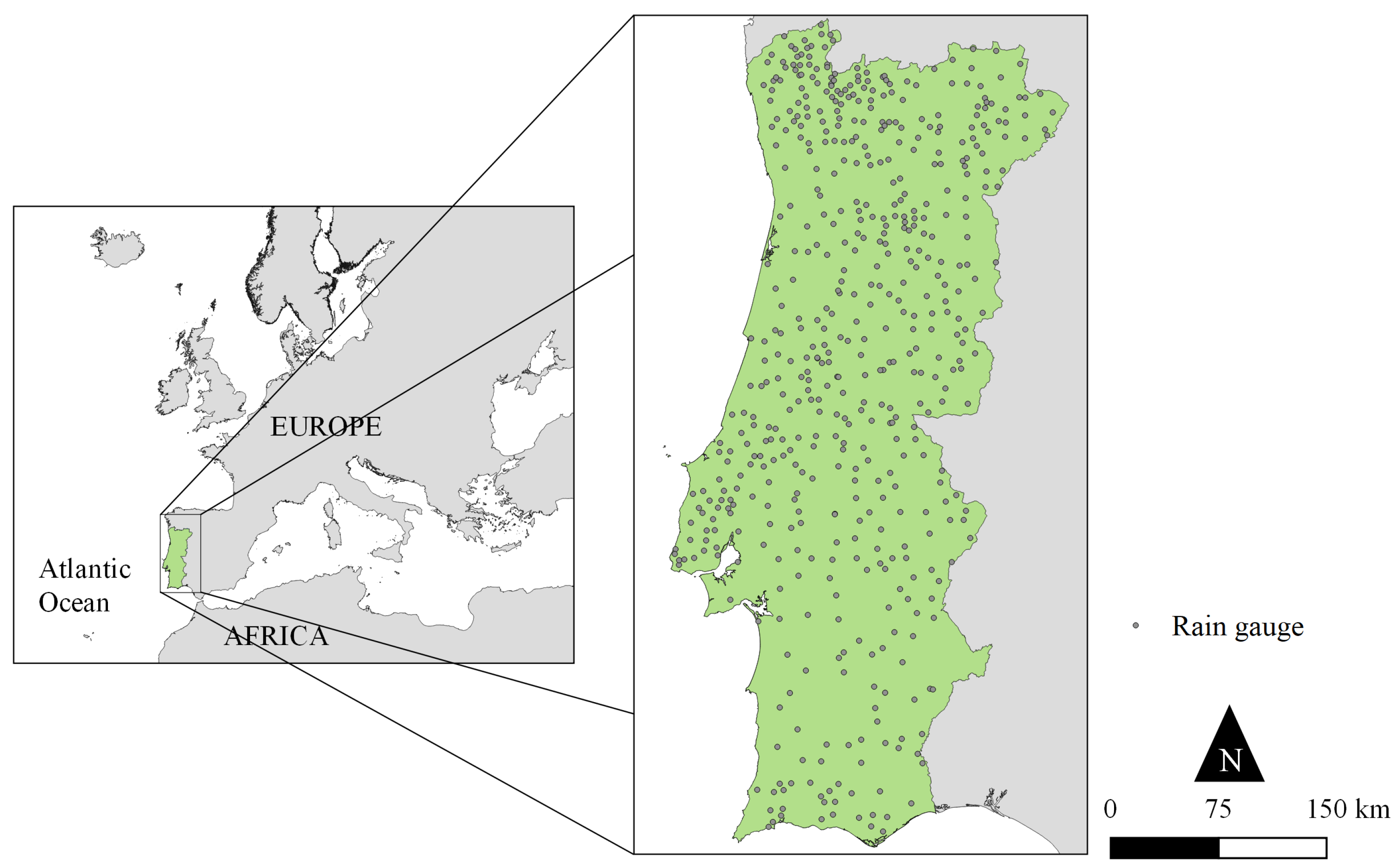
The rainfall trend analysis considered mainland Portugal, with approx. 89,000 km, as study area. The country is in the western part of the Iberian Peninsula (37 to 42 N and 6 to 9.5 W), facing the Atlantic Ocean, in the transitional region between the sub-tropical anticyclone and the subpolar depression zones (Figure 1). The major natural factors that condition the climate of the country are the latitude, the topography, ranging from approx. 0 to 2000 m.a.m.s.l., and the effect of the North Atlantic Ocean as the most eastern regions of the country are only c.a. 220 km away from it [41,42]. The mean annual rainfall over Portugal varies from more than 2800 mm, in the north-western region, to less than 400 mm, in the southern region, following a complex spatial pattern (N–S/E–W), in close connection with the relief [43].
2.2. Rainfall Dataset
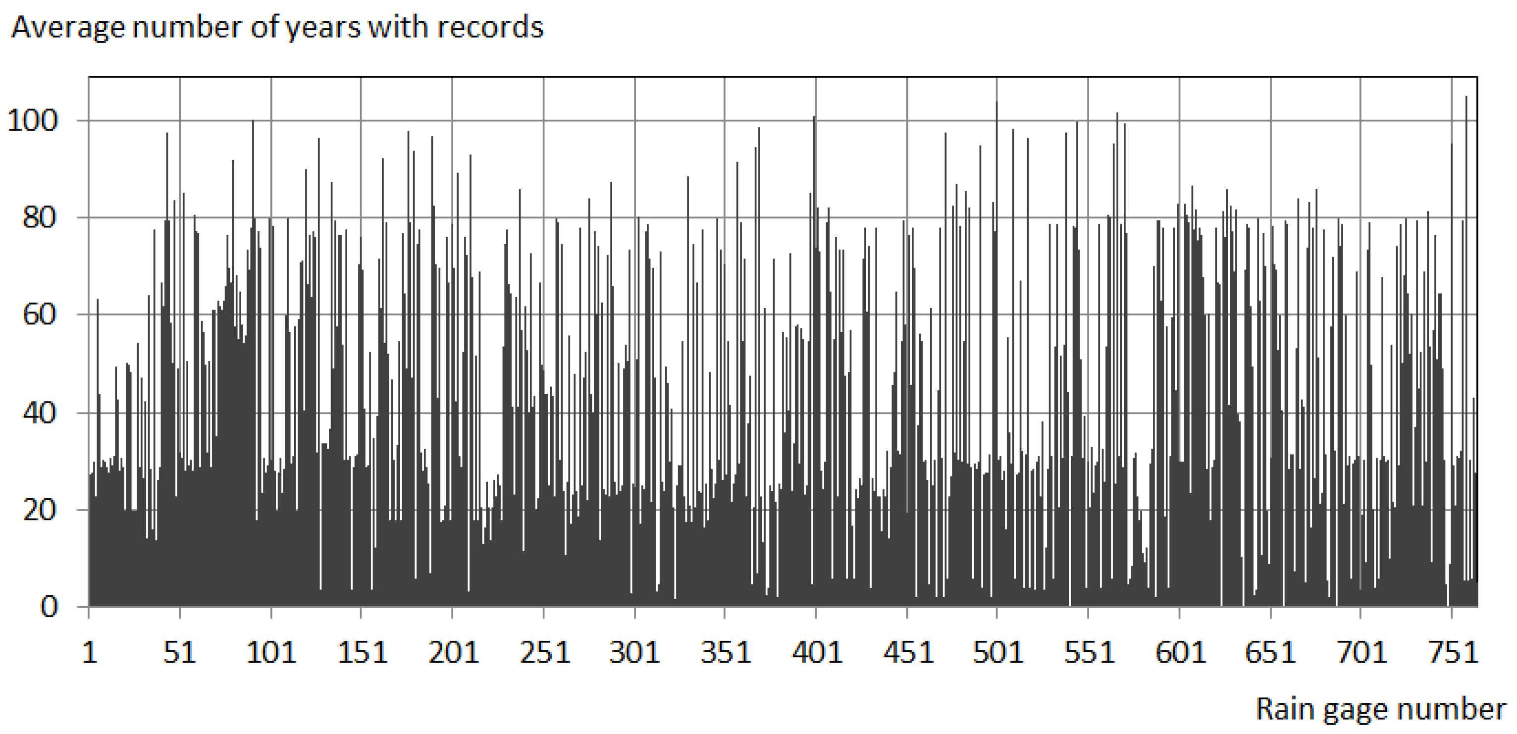
The original rainfall records used in the study span from October 1910 to September 2019 (109 hydrological years, each starting 1 October). The records were acquired from 764 rain gauges of the public database of the Portuguese Environment Agency, the Sistema Nacional de Informação de Recursos Hídricos [44]. All the rain gauges have incomplete series, as briefly characterized in Figure 2 and Figure 3.
Figure 2 shows a histogram of the number of rain gauges per class of number of available monthly records from October 1910 on. The amplitude of the classes is equal to 10, except for the last class whose upper limit coincides with the number of months of the recording period ( months). Figure 3 indicates the average number of years with monthly records in each rain gauge, obtained by dividing the number of available monthly records by 12. The number of rain gauges with, on average, 20, 40 and 60 years with monthly records is 641, 374 and 242, respectively. Although the previous characterization does not provide any information about the regularity of the distribution of the records along the different months, it shows that there is a considerable amount of monthly rainfall series, although with several gaps.
To fill the gaps aiming at obtaining continuous rainfall series a linear regression model based on an each-gap specific equation was applied [26,43]. For a rainfall gap in month m of year n, in a given rain gauge, , the model identifies the candidate rain gauges, , with and , where k is the number of rain gauges, with records in month m of year n and, therefore, that can be used to fill the gap. These gauges are next ranked according to the correlation coefficient between paired rainfall series in month m in years other than n, at the rain gauge with the gap, , and at each of the candidate rain gauges, .
From the candidate rain gauges, the one with the highest correlation coefficient between the previous paired monthly rainfall series is used to fill the gap based on a linear regression model applied to those series, provided two requisites are met: the length of the two paired rainfall series in month m and the correlation coefficient between those series must be higher than prefixed minimum values, so that the regression model is valid and the dependency structure significant. Regarding the length, a minimum value of 15 years was adopted. Because 83 out of the 764 rain gauges had less than 15 rainfall records in any month, they were discarded from the filling-gap procedure, which therefore proceeded with 681 rain gauges.
Regarding the correlation coefficient, two values were considered: 0.7 for the months from October to June, where rainfall is expected to occur in Portugal, and 0.6 for the months from July to September with negligible rainfall amounts (approx. 7% of the annual amount), often due to erratic short duration rainfall events over very small areas. In the establishment of the linear regression models only recorded values are considered (and not the values resulting from the gap filling procedure).
For the period from 1913/1914 to 2018/2019, the previous approach led to 288 rain gauges with complete series and to 244 rain gauges, each with less than 10 monthly gaps. Taking into account the very small number of remaining gaps compared to the number of months or even to the number of years of the period (in each rain gauge, less than 10 months out of months, and less than 1 year, out of 106 years), it was decided to assign the historical monthly averages (i.e., averages prior the gap filling procedure) to those gaps. This resulted in the set of 532 rain gauges schematically located in Figure 1, covering almost uniformly the country (c.a. 6 rain gauges per 1000 km), with continuous monthly rainfall data over a global period of 106 years.
2.3. Long-Term Trend Analysis Models
The well-known rank-based nonparametric Mann-Kendall test was applied to assess the significant trends [45,46]. The adopted significance level was . The magnitude of the monotonic trends was measured based on the Sen’s slope estimator test [47]. A positive value of the Sen’s slope estimator indicates an increasing (or upward) trend and a negative value a decreasing (or downward) trend in the time series.
To produce maps with the spatial variability of the magnitude of the trends at a given time scale, the Sen’s estimator was computed for all the corresponding rainfall time series regardless the statistical significance of the results from Mann-Kendall test.
3. Results
3.1. Rainfall Characterization
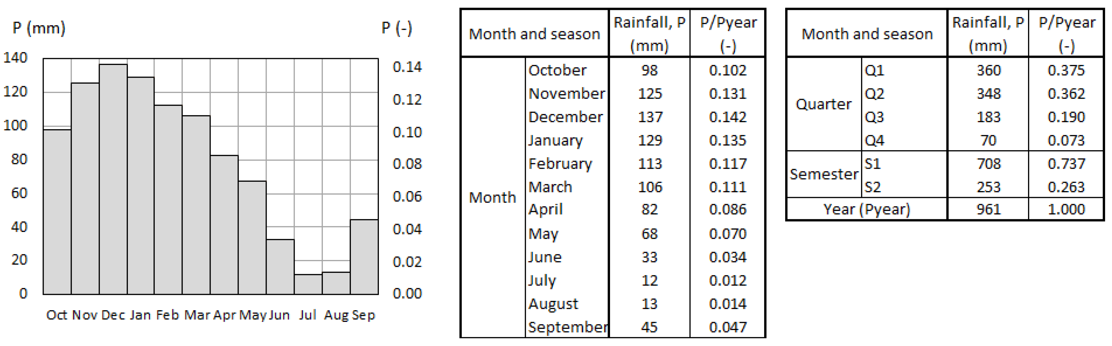
Figure 4 presents a simplified characterization of the intra-annual distribution of the rainfall over mainland Portugal based on the continuous monthly rainfall data at the 532 rain gauges used in the study (Figure 1). Each seasonal rainfall was weighted according to the grid generated by the cubic spline interpolation [48,49]. As the study adopted hydrological years (starting each October and finishing next September), the definition of the quarters, Q, and of the semesters, S, is as follows: Q1—October to December; Q2—January to March; Q3—April to June; Q4—July to September; S1—October to March; and S2—April to September. In the table, the rainfalls are expressed in absolute values and in dimensionless values obtained by dividing the average rainfall in each month and season by the mean annual rainfall that result from the entire set of data, i.e., approx. 961 mm.
According to Figure 4, the average contribution of the wet semester, S1, from October to March, to the annual amount of rainfall is ca. 74%, approximately equally distributed by its two first quarters, Q1 and Q2. The less contributing quarter of the year is the last one, Q4, from July to September, which only accounts for ca. 7% of the mean annual rainfall. These results are in accordance with the rainfall characterization of the National Water Plan [50].
Along with the analysis for the 106-year global period (from 1913/1914 to 2018/2019), two sub-periods were also considered: (i) the initial 55 years, from October 1913 to September 1967, and (ii) the final 51 years, from October 1968 to September 2019. This partition was done to ascertain if the rainfall trends became more pronounced recently, as reported by [26] for southern Portugal. The starting year of the final sub-period coincides with the one previously adopted in the study for the south of the country, based on the application of the Sequential Mann-Kendall test [51,52], although to a period slightly different from the one now adopted (from October 1910 to September 2017). This is also in accordance with the findings by [53], showing that several important characteristics of the global atmospheric circulation and climate changed in a near-monotonic fashion over the decade centered on the late 1960s.
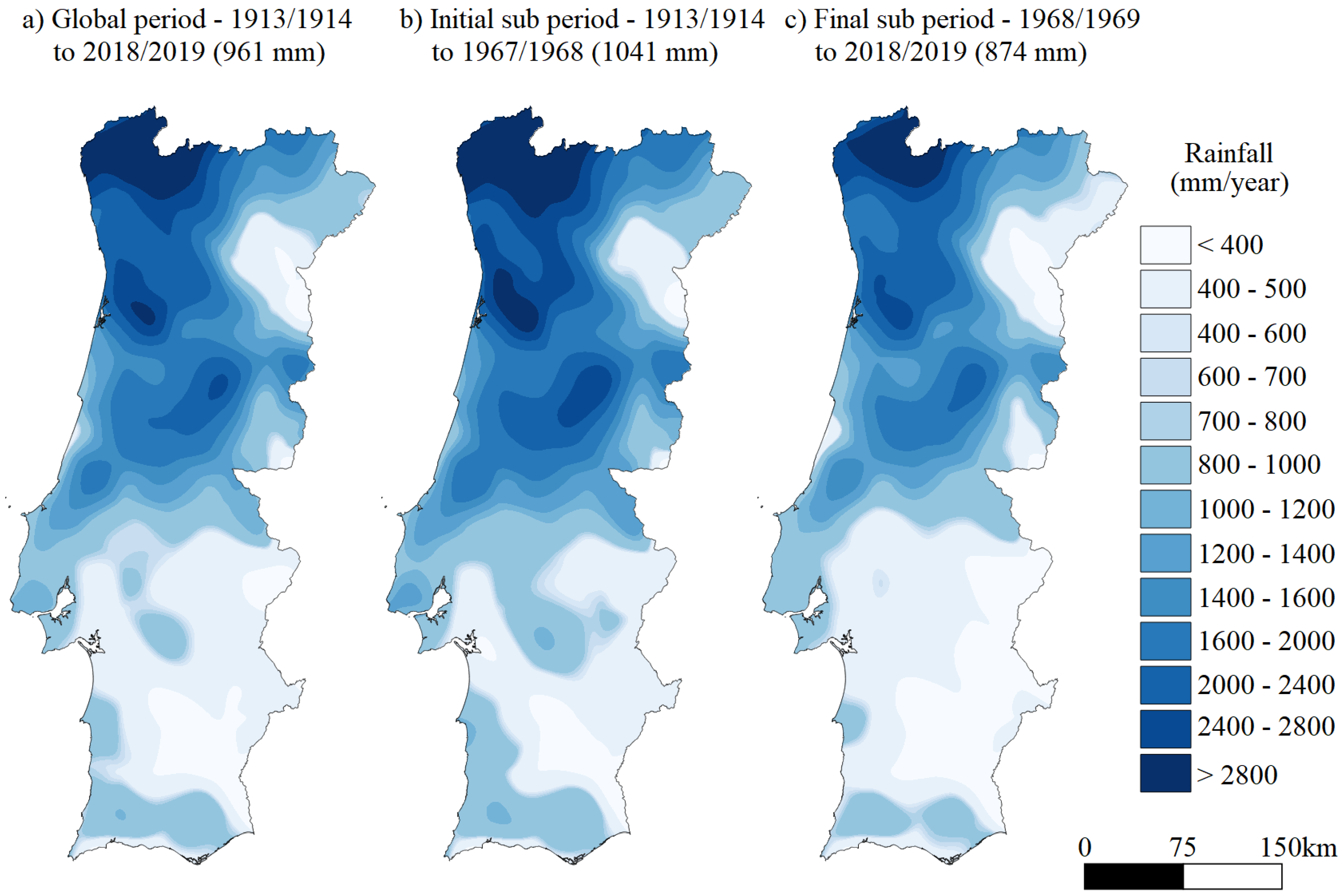
The map of the mean annual rainfall over mainland Portugal derived from the cubic spline interpolation technique applied to the mean annual rainfalls at the 532 rain gauges is presented in Figure 5. Besides the global period, the two previous sub-periods were included for a better perception of the annual rainfall changes. The cubic spline interpolation was applied to the mean annual rainfall in mainland Portugal, because it gives a smoother interpolation, when dealing with high-density rain gauge network, compared to the other interpolation methods [54].
Based on Figure 5 it is easy to follow the spatiotemporal rainfall changes, with generally wetter conditions in the 55-year initial sub-period (Figure 5b) even in the inner southern of Portugal, and drier conditions in the 51-year final sub-period (Figure 5c). The decrease of the mean annual rainfall from one period to the other is almost 170 mm. This affects the whole country, but also emphasizes the asymmetry in the rainfall distribution between the wetter north and the drier south, the latter being recognized as suffering a progressive desertification process [55,56].
3.2. Mann-Kendall Test and Sen’s Slope Estimates
The trends at the 532 rain gauges were characterized via the Mann-Kendall and Sen’s slope estimator tests at the annual level but also at the quarterly (Q1 to Q4) and semi-annual (S1 and S2) timescales aiming to ascertain the intra-annual signs of the climate change [26,57]. For each of the periods and time scales, Table 1 summarizes the number of rain gauges with significant trends and the corresponding extreme (maximum, for increasing trends, and minimum, for decreasing trends) and mean values of the Sen’s slope estimates. The results related to negative (downward) and positive (upward) trends are highlighted in blue and yellow, respectively. Additionally, Figure 6, Figure 7 and Figure 8 present the spatial distribution of the estimates from the the Sen’s slope estimator, regardless their statistical significance.
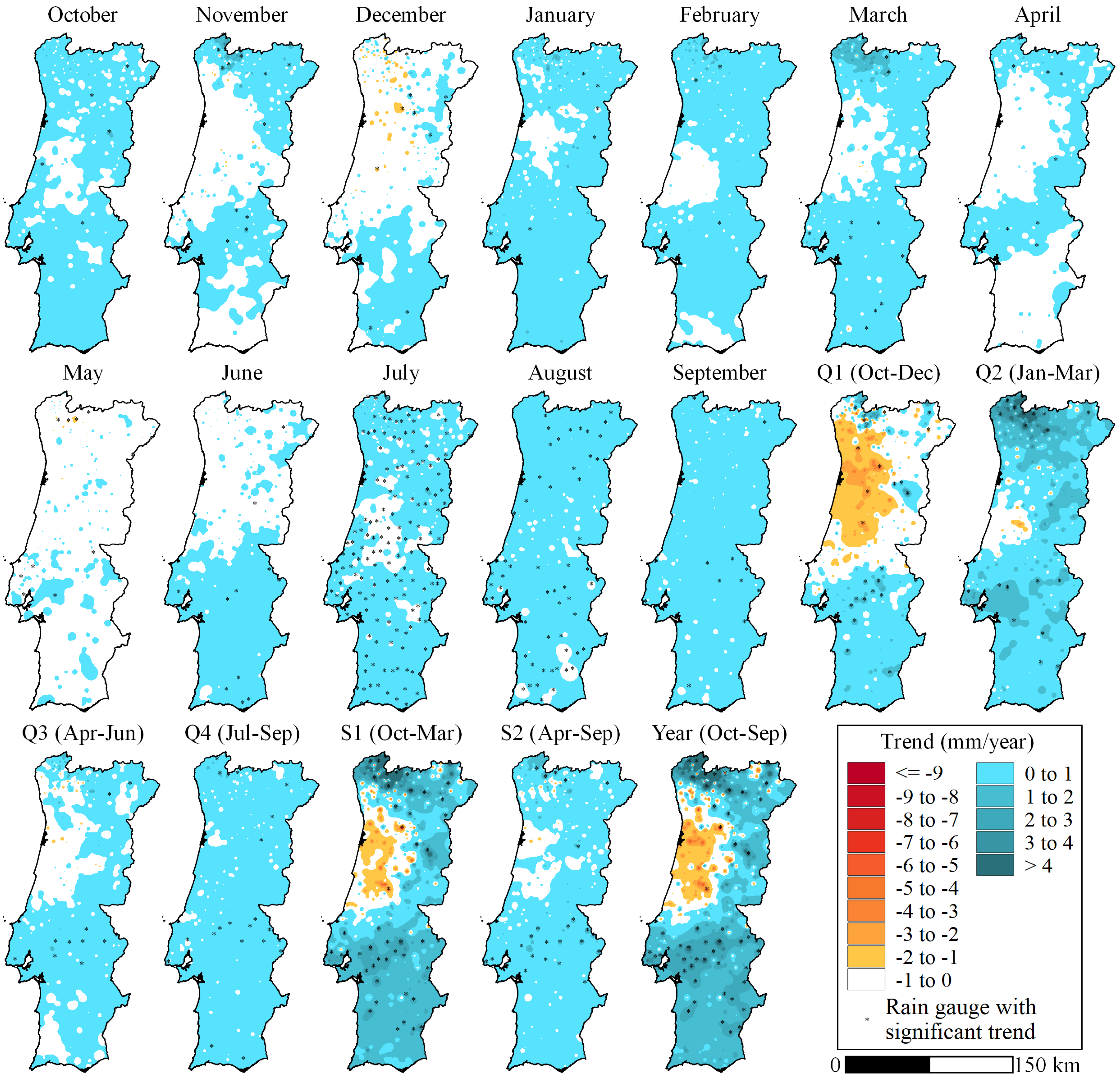
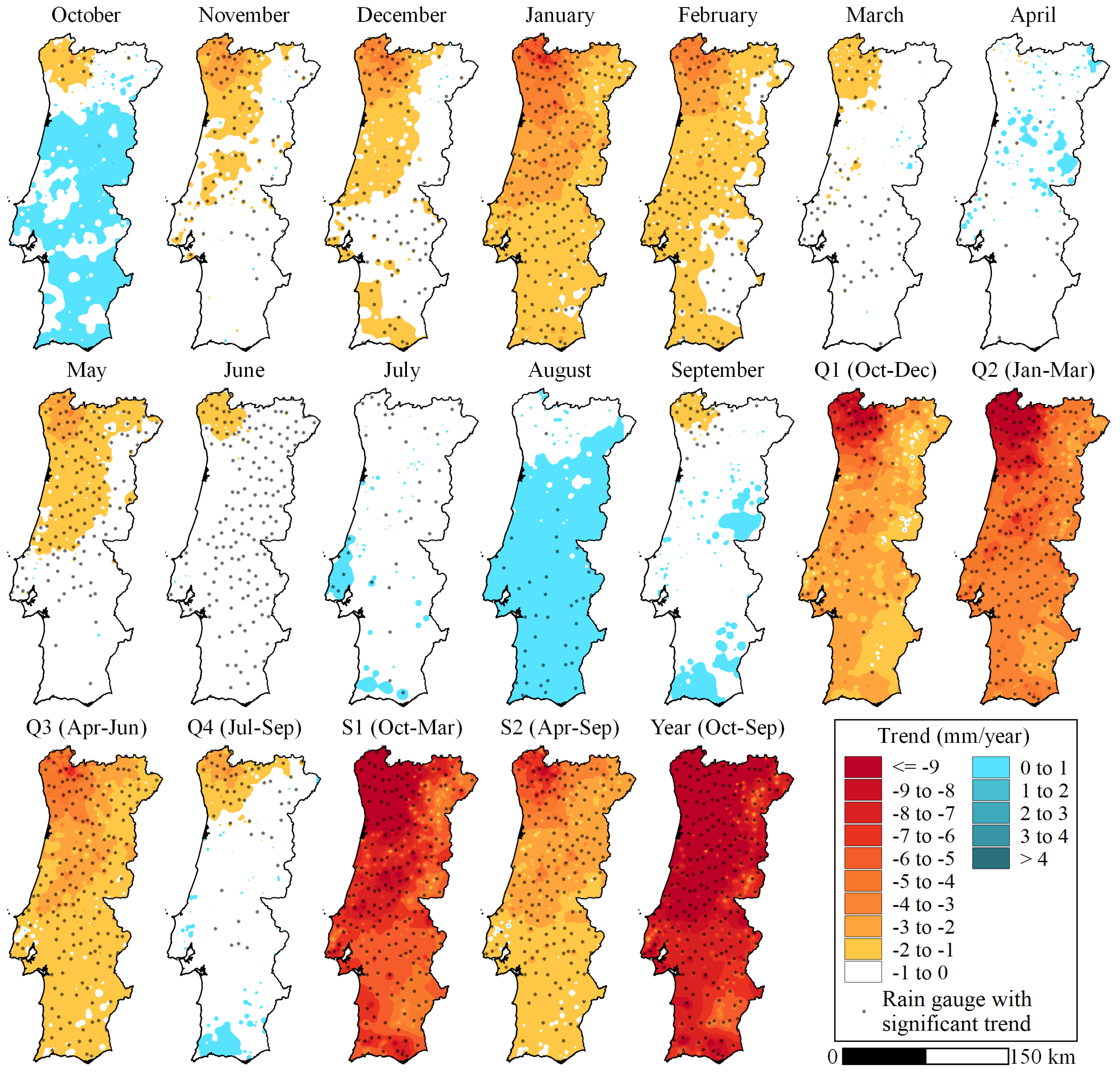
Table 1 clearly indicates that after the initial 55-year period mostly with positive significant rainfall trends, a more recent 51-year period almost exclusively with negative significant trends occurred. The only exception are the summer months of July and August, which nevertheless have very small contributions to the annual rainfall (1.2 and 1.4%, respectively—Figure 4). The negative trends in the final sub-period were so pronounced that they counterbalanced the positive trends in the first period and resulted in more frequent negative trends for the whole period, albeit less marked. This is the case, for instance, of the annual rainfall with 505 rain gauges with a mean significant downward trend of −11.42 mm/year in the final sub-period, whereas the equivalent numbers for the global period are 428 and −4.27 mm/year, respectively. These rainfall trends are aligned with the results of [26] for the south of Portugal.
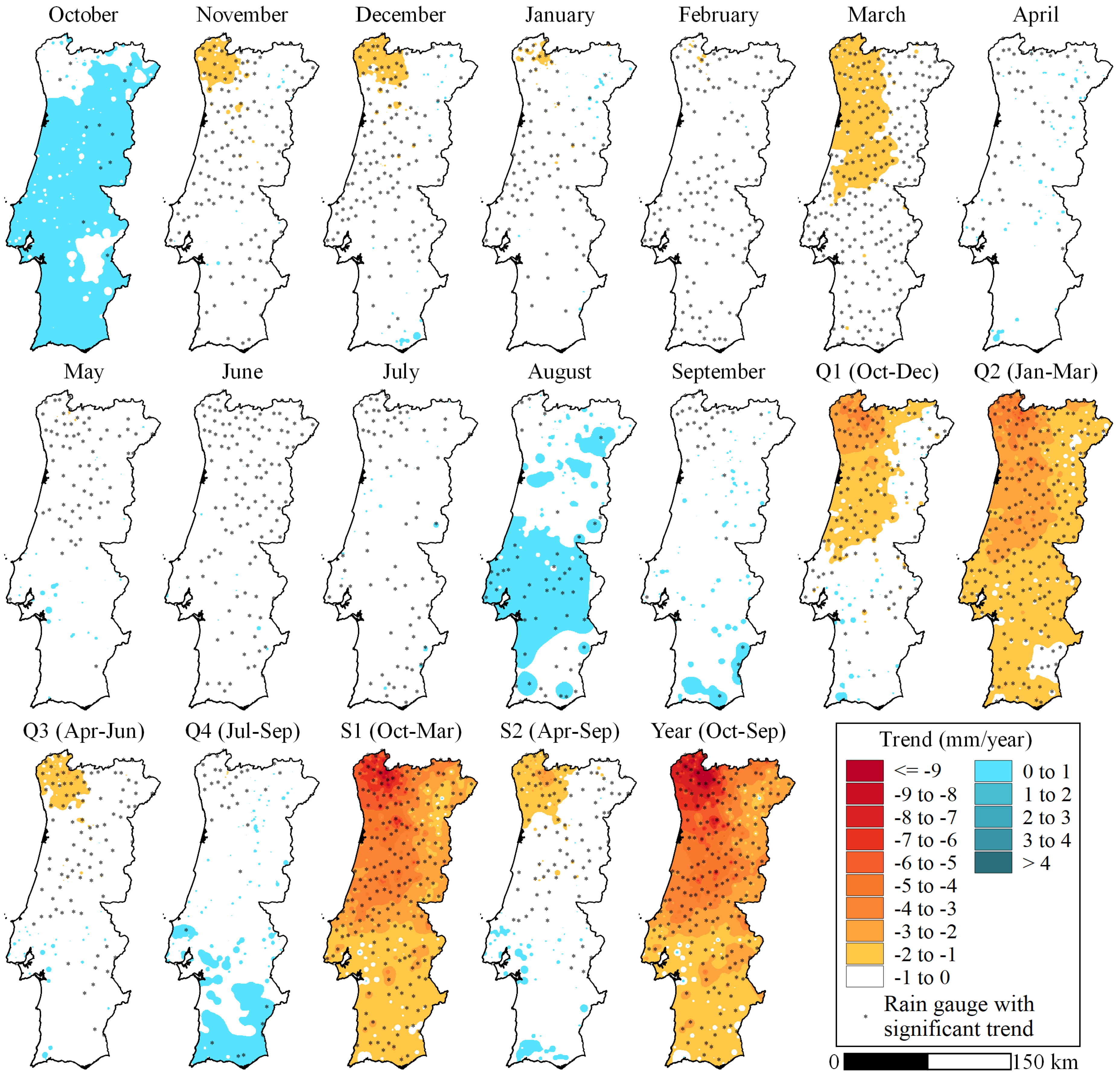
The comparison of Figure 6, Figure 7 and Figure 8 reinforces the results reported in Table 1 by highlighting the exceptional and, for some timescales, widespread extent of the decreasing trends in the last 51 years, especially in contrast with the initial 55 years. The results for the quarters, semesters and year are especially marked, with reduction of the rainfall in some rain gauges often greater than 9 mm/year in the last 51 years. The figures also point out some important information regarding the monthly distribution of the rainfall. In fact, when looking at the 106-year global period, March appears as the month with the highest number of significant and pronounced trends. However, when considering the most recent sub-period it is notorious that the more noticeable trends occur in the months before, namely in January and especially in February. The shift between February and March is also evident based on the number of rain gauges with significant decreasing trends, as reported in Table 1: for the global period, 189 in February and 517 in March; the equivalent values for the last 51 years are 479 and 353. These results suggest that the decrease of the rainfall is moving “backwards” and progressively affecting the months before March.
The identified “backwards” behavior resulted in aggravated decreasing rainfall trends in the last 51 years compared to the global period. For Q2, i.e., from January to March, the average decrease of the rainfall in the last sub-period is 2.4 times the one in the global period (−5.26 mm/year versus −2.15 mm/year), despite having the same number of rain gauges with significant trends (492).
A comparison for the remaining quarters between the last 51 years and the 106-year global period shows the noteworthy aggravation in the rainfall decrease in Q1 (−6.00 mm/year versus −2.15 mm/year) and in the increase of the number of rain gauges with significant trends for both Q3 (372 versus 193) and Q4 (127 versus 73). In these two last quarters, an aggravation in the rainfall decrease also occurs (with absolute values of the trends approx. 2.6 and 3.2 times more, respectively), although with less pronounced decreases in terms of the rainfall itself.
Regarding the semesters, the ratio between average trends in the last 51 years and in the global period is approx. 2.4, clearly showing more pronounced rainfall decreases. The aggravation in the rainfall decrease in S1 (−8.74 mm/year versus −3.61 mm/year) and the increase in the number of rain gauges with significant trends in S2 (399 versus 189) should also be stressed. The comparison for the annual rainfall shows an increase in the number of rain gauges with significant trends (505 versus 428 rain gauges) and an aggravation in the averages of those trends (−11.42 mm/year versus −4.27 mm/year).
3.3. Sequential Variability of the Rainfall
To understand the intra-annual behavior of the rainfall, a complementary approach, namely the simple moving average technique, was applied to the weighted rainfalls at the 532 rain gauges for the different timescales based on a running length of years. The weight assigned to each rain gauges was given by the Voronoi or Thiessen polygons [58,59]. For the global period of 106 years, the number of moving averages for each time scale is .
The moving average technique allows to smooth out of short-term fluctuations and to highlight longer-term trends or cycles in a long temporal series [60]. Periods of 30 years (as considered for the running length) are also adopted in the computation of the climatological standard normals aiming at to ascertain the climatic conditions likely to be experienced in a given location [61,62].
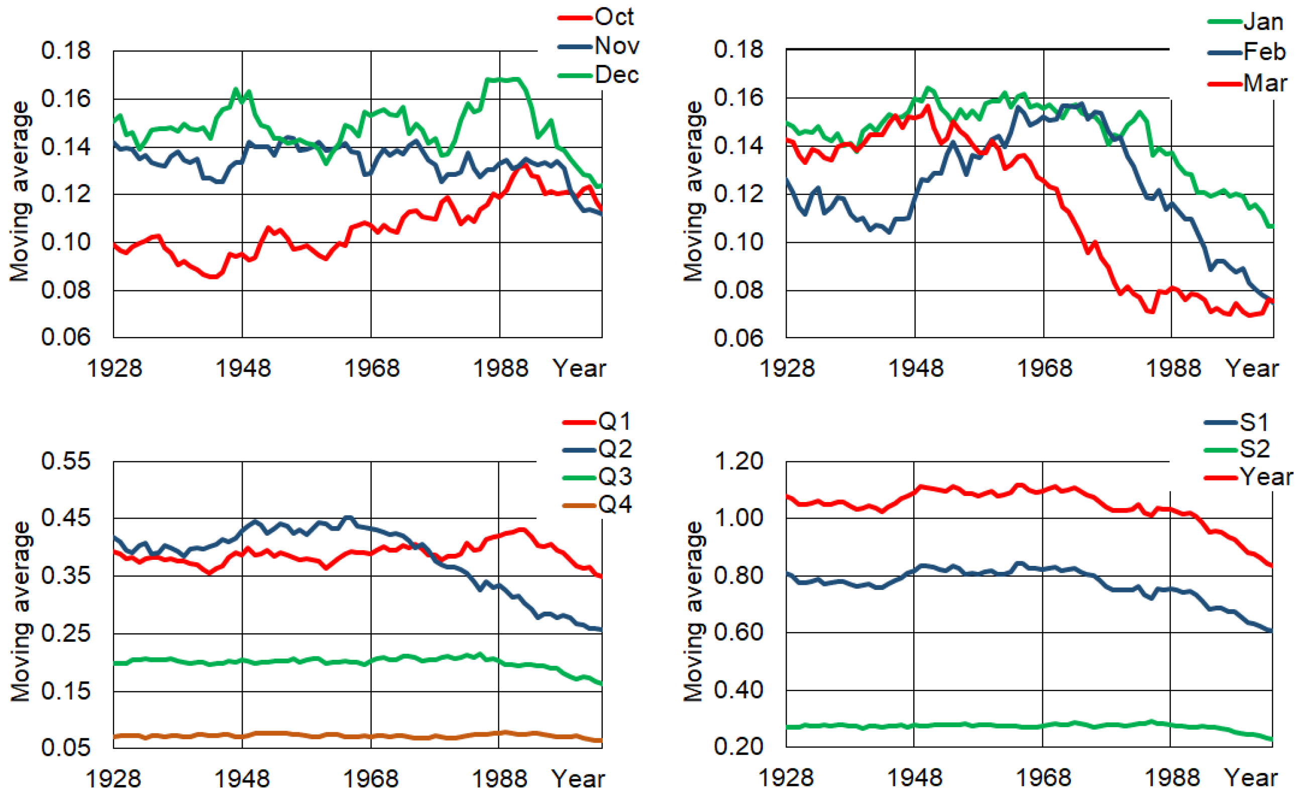
Figure 9 shows the results for the six initial months, the quarters, and the semesters of the hydrological year, and for this year itself. The results for the months of the dry semester, from April to September, were not represented due to their small contribution to the annual rainfall amount (approx. 26%). The rainfalls at the different timescales were made comparable by dividing them by the mean annual rainfall of 961 mm presented in Figure 4. In Figure 9 each moving average was assigned to the first civil year of the 16th hydrological year of the corresponding 30-year period (first moving average from 1913/1914 to 1942/1943 assigned to 1928 and last moving average from 1989/90 to 2019/2019 assigned to 2004).
For the quarterly, semi-annual and annual timescales, Figure 9 shows the decreasing behavior of the rainfall towards the present. The downward trends are particularly marked in the wet season (Q1, Q2 and S1), which explains the trends at the annual level. Due to the prevailing Mediterranean-type climatic conditions in Portugal, the wet season rainfall amount is the determining factor in the water budgets of the hydrological cycle, namely in terms of the natural and artificial storage replenishment. This season also plays a key role in triggering drought episodes, because the environmental and socio-economic systems are not prepared for an unexpected lack of winter rainfall, although they are to cope with the natural summer dryness [27].
The last three months of the wet season (i.e., Q2, from January to March) bring out new insights into the previous behavior. In fact, the rainfall decrease in March—particularly noticeable in the moving averages of the 30-year periods from 1940/1941 on—seems to have stabilized after the periods starting in 1970/1971, albeit with values much smaller than the long-term historical average. The pronounced decreasing rainfall tendency in March seems to have “moved” backwards affecting the months of January and February. Such “displacement” is particularly evident in the moving averages starting on the late years (in the case of January) and on the early years (in the case of February) of the decade beginning in 1970/1971, clearly indicating that the intra-annual rainfall pattern is changing. These downward trends seem to be sustained in recent years, resulting, for instance, in an average rainfall from January to March in the last 30-year period (1989/1990 to 2018/2019) of 246 mm, i.e., ca. 71% of the long-term average of 348 mm and 61% of the average of 402 mm in the first 30-year period of the moving averages (1913/1914 to 1942/1943). The more pronounced decreasing trends detected for the final sub-period, from 1967/1968 on (Figure 8), are also visible in the moving averages along the same period, which in Figure 9 are assigned to the years from 1982 on (i.e., 1967 + 15).
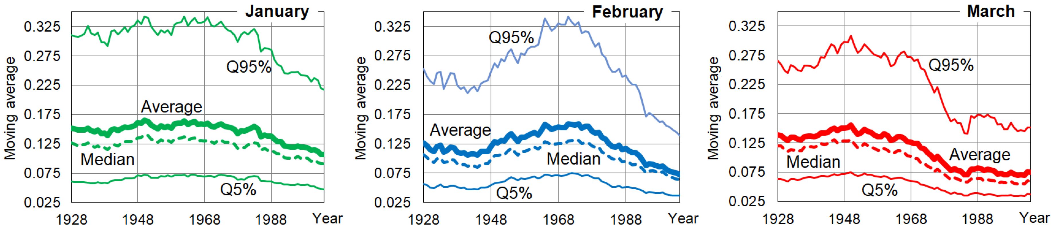
For each of the months from January to March, during which the intra-annual pattern of the rainfall is changing, an additional analysis was done based on the moving averages of the rainfalls at the set of 532 individual rain gauges instead of considering only spatially weighted rainfalls. In this respect, each set of 532 moving averages referred to a same year (from 1913/1914 to 1989/1990, starting years of the first and last 30-year moving averages, respectively) was characterized by the corresponding median, average, and empirical quantiles for the non-exceedance probabilities of 5% (Q5%), and 95% ( Q95%), as shown in Figure 10. The averages curves of this figure coincide with those of Figure 9.
For any month of Figure 10, there is always a great dispersion of the moving average values in the set of 532 rain gauges. Along the years, the averages are always higher than the corresponding medians, and the Q95% values are much higher than the averages, while the Q5% values are closer to the averages. This means that (i) the data is skewed to the left, (ii) there is a long tail of low scores on the right side of the empirical distributions, and (iii) there are a few exceptional high values “pushing up” the averages. The results for the set of 532 rain gauges confirm the behavior towards the present previously stressed for March, i.e., a stabilizing tendency around much smaller values than the long-term averages. For February and January, it is also notorious a “dynamic” behavior, with markedly decreasing tendencies which are apparently still ongoing and with no further stabilization. The figure also shows that the amplitude between the quantiles Q95% and Q5% is consistently decreasing as the moving averages relate to more recent periods. Such decrease indicates less variability in the rainfall behavior within the set of 532 rain gauges, and accordingly, less uncertainty in the overall expected decrease of the rainfall over Portugal.
4. Discussion and Conclusions
Understanding past rainfall variations and being able to anticipate the expected rainfall changes over different time scales are of utmost importance because the hydrological processes driven by the rainfall (e.g., evapotranspiration and surface and ground water flow) affect the whole water resources system. The analysis of ground-based rainfall observations can help to comply with such purposes given the corresponding series are updated, long enough [28], and supported by a dense monitoring network able of describing the spatial rainfall variability [29]. This is the case of the present research work which to the authors’ best knowledge represents the most thorough and comprehensive study on rainfall trends over mainland Portugal, using ground-based data, addressing the long-term monthly, seasonal and annual rainfall changes and the recent rainfall trends dynamics.
This study shows that in the last five decades the rainfall has been markedly decreasing over mainland Portugal. Such decrease has been progressively affecting the more contributing months of the wet season, in absolute terms but also regarding their relative contribution to annual rainfall, thus strongly conditioning the intra-annual rainfall pattern. This behavior is particularly pronounced before the long dry season start, i.e., in the last wet period of the hydrological year (Q2, January to March), a fundamental period for the replenishing of the water, both in the soil and in the artificial reservoirs. The analysis of the set of 532 rain gauges throughout the 106-year period showed that the amplitude of the rainfall decrease has gradually narrowed, meaning less uncertainty about its behavior.
When considering the global 106-year period, but especially the most recent 51-year sub-period, from 1968/1969 on (Figure 5 and Figure 8), the study revealed a coherent monthly spatial pattern of the trends, with each month showing almost a same rainfall trend over the country. For the months of the rainy season, except for October, the trends are consistently negative. Such homogeneous behavior indicates the vulnerability of the country to the rainfall decrease given it is not expected that some regions may become wetter, thus counterbalancing those becoming drier.
To understand the relevance of the previous vulnerability, rainfall anomalies were assigned to each rain gauge and spatially represented based on the cubic spline interpolation (Figure 11). In each rain gauge, the anomaly was defined as the mean annual rainfall in the last 51 years minus the mean annual rainfall in the initial 55 years. Each anomaly was expressed in absolute terms (Figure 11a) and made dimensionless (Figure 11b), by dividing by the average in the initial period (dimensionless anomaly relative to the 55-year initial period).
Figure 11a shows that except for very small regions, the country experienced a mean annual rainfall decrease from one sub-period to another above 120 mm. In the northwest wettest region such decreases exceeds 500 mm. Figure 11b allows understanding of the relevance of the magnitude of those results. It shows that a same dimensionless rainfall reduction affects both wetter and drier regions meaning that some of these last regions are becoming much drier than the former ones. Such behavior reinforces the difference between a less wet, yet wetter, north and a definitely drier arid south. This agrees with the findings of the global assessment of wetting/drying trends during the period 1948–2005 of Greve et al. [63] that identified the southwest regions of the Iberian Peninsula as one hot spot of the pattern “dry gets drier” (the DD paradigm).
The recent rainfall reduction, from late 1960 on, portraited in Figure 11, agrees with the widespread drying tendency across North Africa and southern Europe, extending from the Atlantic coast to the Middle East, detected by Hoerling et al. [64] when comparing the periods 1902–1970 and 1971–2010.
The rainfall tendency to decrease in sub-tropical latitudes mentioned in some IPCC reports [4,5,6], has been verified in this case for Portugal despite the complex spatial and temporal rainfall distribution. This agreement was achieved with the use of spatially dense long-running rainfall series rarely available with the necessary resolution compared to general low resolution global atmosphere reanalysis datasets—such as the Multi-Source Weighted-Ensemble Precipitation (MSWEP) global dataset from 1979 to 2015 [65]. Although ground-based rainfall data analysis and reanalysis normally exhibit differences due to the different inferential processes and resolution [66], a comparison between the here obtained trends and those via global model reanalysis datasets [67], shows a consistent rainfall reduction from December to March in recent years. However, these findings need to be interpreted with caution depending on the data source used. The results for the final sub-period are also in accordance with a study based on downscaling [68], denoting a significant decrease in the rainfall amount in certain regions of the Iberian Peninsula during the last third of the 20th century.
Despite it is difficult to make a global synthesis of the results obtained from the different observation periods, data, methods implemented, etc., there is prima-facie evidence about the generalized rainfall decrease in Portugal. This is reinforced by the global evidence, based on likely emission scenarios [69], of a future with less freshwater availability in sub-tropical latitudes. It also stresses the urge for widespread public awareness and participation towards common water-saving practices. Public participation is a key factor, also because it calls for updated information and political commitment towards the implementation of mitigation and adaptation measures and of new water resources planning and management policies. Both challenges are presently far from being achieved for mainland Portugal [70].
Author Contributions
Conceptualization, M.M.P.; methodology, M.M.P.; software, L.A.E., M.M.P.; validation, L.A.E.; formal analysis, L.A.E., M.M.P.; investigation, M.M.P.; resources, M.M.P.; data curation, L.A.E., M.M.P.; writing—original draft preparation, M.M.P.; writing—review and editing, L.A.E., M.M.P.; visualization, L.A.E.; supervision, M.M.P., M.Z. All authors have read and agreed to the published version of the manuscript.
Funding
This research received no external funding.
Acknowledgments
This work is funded by the Portuguese Foundation for Science and Technology (FCT), Scientific Cooperation Agreement between Portugal and Slovakia–2019/2020, SK-PT-18-0008, regarding the first and third authors; and by FCT grant No. PD/BD/128509/2017, as for the second author.
Conflicts of Interest
The authors declare no conflict of interest.
References
- Briffa, K.; Van Der Schrier, G.; Jones, P. Wet and dry summers in Europe since 1750: Evidence of increasing drought. Int. J. Climatol. J. R. Meteorol. Soc. 2009, 29, 1894–1905. [Google Scholar] [CrossRef]
- Donat, M.G.; Lowry, A.L.; Alexander, L.V.; O’Gorman, P.A.; Maher, N. More extreme precipitation in the world’s dry and wet regions. Nat. Clim. Chang. 2016, 6, 508–513. [Google Scholar] [CrossRef]
- Pfahl, S.; O’Gorman, P.A.; Fischer, E.M. Understanding the regional pattern of projected future changes in extreme precipitation. Nat. Clim. Chang. 2017, 7, 423–427. [Google Scholar] [CrossRef]
- McCarthy, J.J.; Canziani, O.F.; Leary, N.A.; Dokken, D.J.; White, K.S. Climate Change 2001: Impacts, Adaptation, and Vulnerability: Contribution of Working Group II to the Third Assessment Report of the Intergovernmental Panel on Climate Change; Cambridge University Press: Cambridge, UK; New York, NY, USA, 2001; Volume 2. [Google Scholar]
- Parry, M.; Parry, M.L.; Canziani, O.; Palutikof, J.; Van der Linden, P.; Hanson, C. Climate Change 2007: Impacts, Adaptation and Vulnerability: Working Group II Contribution to the Fourth Assessment Report of the Intergovernmental Panel on Climate Change; Cambridge University Press: Cambridge, UK; New York, NY, USA, 2007; Volume 4. [Google Scholar]
- Barros, V.; Field, C.; Dokke, D.; Mastrandrea, M.; Mach, K.; Bilir, T.E.; Chatterjee, M.; Ebi, K.; Estrada, Y.; Genova, R.; et al. Climate Change 2014: Impacts, Adaptation, and Vulnerability-Part B: Regional Aspects-Contribution of Working Group II to the Fifth Assessment Report of the Intergovernmental Panel on Climate Change; Cambridge University Press: Cambridge, UK; New York, NY, USA, 2014. [Google Scholar]
- Bates, B.; Kundzewicz, Z.; Wu, S. Climate Change and Water; Intergovernmental Panel on Climate Change IPCC Secretariat: Geneva, Switzerland, 2008. [Google Scholar]
- Khan, M.Z.K.; Sharma, A.; Mehrotra, R. Global seasonal precipitation forecasts using improved sea surface temperature predictions. J. Geophys. Res. Atmos. 2017, 122, 4773–4785. [Google Scholar] [CrossRef]
- López-Moreno, J.I.; Vicente-Serrano, S.M.; Gimeno, L.; Nieto, R. Stability of the seasonal distribution of precipitation in the Mediterranean region: Observations since 1950 and projections for the 21st century. Geophys. Res. Lett. 2009, 36. [Google Scholar] [CrossRef] [Green Version]
- Muñoz, J.M.H. Assessing the Impact of Climate Variability on Seasonal Streamflow Forecasting in the Iberian Peninsula. Ph.D. Thesis, Universidad de Granada, Granada, Spain, 2015. [Google Scholar]
- Ojeda, M.M.d.V.G.V. Climate-Change Projections in the Iberian Peninsula: A Study of the Hydrological Impacts. Ph.D. Thesis, Universidad de Granada, Granada, Spain, 2018. [Google Scholar]
- Soares, P.M.; Cardoso, R.M.; Ferreira, J.J.; Miranda, P.M. Climate change and the Portuguese precipitation: ENSEMBLES regional climate models results. Clim. Dyn. 2015, 45, 1771–1787. [Google Scholar] [CrossRef]
- Miranda, P.; Coelho, F.; Tomé, A.R.; Valente, M.A.; Carvalho, A.; Pires, C.; Pires, H.O.; Pires, V.C.; Ramalho, C. 20th century Portuguese climate and climate scenarios. Climate Change in Portugal. Scenarios, Impacts and Adaptation Measures—SIAM Project; Santos, F.D., Forbes, K., Moita, R., Eds.; Gradiva Publishers: Lisbon, Portugal, 2002; pp. 23–83. [Google Scholar]
- Santos, F.D.; Forbes, K.; Moita, R. Climate change in Portugal: Scenarios, Impacts and Adaptation Measures: SIAM Project. In Gradiva; S. Fischer Verlag: Frankfurt, Germany, 2002. [Google Scholar]
- Santos, F.D.; Miranda, P. Alterações Climáticas em Portugal. Cenários, Impactos e Medidas de Adaptação: Projecto SIAM II-1ª Edição; Unidade de Silvicultura e Produtos Florestais: Lisboa, Portugal, 2006; Volume 14, p. 281. [Google Scholar]
- Santo, F.E.; Ramos, A.M.; de Lima, M.I.P.; Trigo, R.M. Seasonal changes in daily precipitation extremes in mainland Portugal from 1941 to 2007. Reg. Environ. Chang. 2014, 14, 1765–1788. [Google Scholar] [CrossRef]
- Gibelin, A.L.; Déqué, M. Anthropogenic climate change over the Mediterranean region simulated by a global variable resolution model. Clim. Dyn. 2003, 20, 327–339. [Google Scholar] [CrossRef]
- Giorgi, F.; Lionello, P. Climate change projections for the Mediterranean region. Glob. Planet. Chang. 2008, 63, 90–104. [Google Scholar] [CrossRef]
- Norrant, C.; Douguédroit, A. Monthly and daily precipitation trends in the Mediterranean (1950–2000). Theor. Appl. Climatol. 2006, 83, 89–106. [Google Scholar] [CrossRef]
- De Luis, M.; Gonzalez-Hidalgo, J.C.; Longares, L.A.; Stepanek, P. Seasonal precipitation trends in the Mediterranean Iberian Peninsula in second half of 20th century. Int. J. Climatol. 2009, 29, 1312–1323. [Google Scholar] [CrossRef]
- Philandras, C.; Nastos, P.; Kapsomenakis, J.; Douvis, K.; Tselioudis, G.; Zerefos, C. Long term precipitation trends and variability within the Mediterranean region. Nat. Hazards Earth Syst. Sci. 2011, 11, 3235. [Google Scholar] [CrossRef] [Green Version]
- Fernández-Montes, S.; Rodrigo, F.S.; Seubert, S.; Sousa, P.M. Spring and summer extreme temperatures in Iberia during last century in relation to circulation types. Atmos. Res. 2013, 127, 154–177. [Google Scholar] [CrossRef]
- Lionello, P.; Abrantes, F.; Gacic, M.; Planton, S.; Trigo, R.M.; Ulbrich, U. The climate of the Mediterranean region: Research progress and climate change impacts. Reg. Environ. Chang. 2014, 14, 1679–1684. [Google Scholar] [CrossRef]
- Andrade, C.; Belo-Pereira, M. Assessment of droughts in the Iberian Peninsula using the WASP-Index. Atmos. Sci. Lett. 2015, 16, 208–218. [Google Scholar] [CrossRef]
- Páscoa, P.; Gouveia, C.; Russo, A.; Trigo, R.M. Drought trends in the Iberian Peninsula over the last 112 years. Adv. Meteorol. 2017, 2017. [Google Scholar] [CrossRef] [Green Version]
- Portela, M.M.; Espinosa, L.A.; Studart, T.; Zelenakova, M. Rainfall Trends in Southern Portugal at Different Time Scales. In International Congress on Engineering and Sustainability in the XXI Century; Springer: Cham, Switzerland, 2019; pp. 3–19. [Google Scholar]
- Santos, J.; Corte-Real, J.; Leite, S. Weather regimes and their connection to the winter rainfall in Portugal. Int. J. Climatol. J. R. Meteorol. Soc. 2005, 25, 33–50. [Google Scholar] [CrossRef]
- Cubasch, U.; Wuebbles, D.; Chen, D.; Facchini, M.C.; Frame, D.; Mahowald, N.; Winther, J.G. Introduction. In Climate Change 2013: The Physical Science Basis. Contribution of Working Group I to the Fifth Assessment Report of the Intergovernmental Panel on Climate Change; Cambridge University Press: Cambridge, UK, 2014. [Google Scholar]
- Girons Lopez, M.; Wennerström, H.; Nordén, L.Å.; Seibert, J. Location and density of rain gauges for the estimation of spatial varying precipitation. Geogr. Ann. Ser. Phys. Geogr. 2015, 97, 167–179. [Google Scholar] [CrossRef] [Green Version]
- Portela, M.M.; Carvalho Quintela, A.D. Indícios de mudança climática em séries de precipitação em Portugal Continental. Recur. Hídricos 1998, 19, 41–74. [Google Scholar]
- Portela, M.M.; Carvalho Quintela, A.d. A diminuiçào da precipitaçào em épocas do año como indício de mudança climática: Casos estudiados em Portugal continental. Ing. Agua 2001, 8, 79–92. [Google Scholar] [CrossRef]
- De Lima, M.I.P.; Marques, A.C.; de Lima, J.; Coelho, M. Precipitation trends in mainland Portugal in the period 1941–2000. IAHS Publ. 2007, 310, 94. [Google Scholar]
- Rodrigo, F.; Trigo, R.M. Trends in daily rainfall in the Iberian Peninsula from 1951 to 2002. Int. J. Climatol. J. R. Meteorol. Soc. 2007, 27, 513–529. [Google Scholar] [CrossRef]
- Santos, J.F.; Portela, M.M. Quantificação de tendências em séries de precipitação mensal e anual em Portugal Continental. In Seminário Ibero-Americano Sobre Sistemas de Abastecimento Urbano (SEREA); SEREA: Lisboa, Portugal, 2008; Volume 8. [Google Scholar]
- De Lima, M.; Carvalho, S.; de Lima, J. Investigating annual and monthly trends in precipitation structure: An overview across Portugal. Nat. Hazards Earth Syst. Sci. 2010, 10, 2429. [Google Scholar] [CrossRef] [Green Version]
- De Lima, M.; Carvalho, S.; de Lima, J.; Coelho, M. Trends in precipitation: Analysis of long annual and monthly time series from mainland Portugal. Adv. Geosci. 2010, 25. [Google Scholar] [CrossRef] [Green Version]
- De Lima, M.I.P.; Santo, F.E.; Ramos, A.M.; Trigo, R.M. Trends and correlations in annual extreme precipitation indices for mainland Portugal, 1941–2007. Theor. Appl. Climatol. 2015, 119, 55–75. [Google Scholar] [CrossRef]
- Portela, M.M.; Santos, J.F.; Silva, A. Trends in rainfall and streamflow series: Portuguese case studies. Int. J. Saf. Secur. Eng. 2014, 4, 221–248. [Google Scholar] [CrossRef]
- Nunes, A.; Lourenço, L. Precipitation variability in Portugal from 1960 to 2011. J. Geogr. Sci. 2015, 25, 784–800. [Google Scholar] [CrossRef]
- Pereira, L.S.; Louro, V.; Do Rosário, L.; Almeida, A. Desertification, territory and people, a holistic approach in the Portuguese context. In Desertification in the Mediterranean Region. A Security Issue; Springer Science & Business Media: Berlin, Germany, 2006; pp. 269–289. [Google Scholar]
- Trigo, R.M.; DaCamara, C.C. Circulation weather types and their influence on the precipitation regime in Portugal. Int. J. Climatol. J. R. Meteorol. Soc. 2000, 20, 1559–1581. [Google Scholar] [CrossRef]
- Belo-Pereira, M.; Dutra, E.; Viterbo, P. Evaluation of global precipitation data sets over the Iberian Peninsula. J. Geophys. Res. Atmos. 2011, 116. [Google Scholar] [CrossRef]
- Santos, J.F.; Pulido-Calvo, I.; Portela, M.M. Spatial and temporal variability of droughts in Portugal. Water Resour. Res. 2010, 46. [Google Scholar] [CrossRef] [Green Version]
- SNIRH. Sistema Nacional de Informação de Recursos Hídricos (2020): APA—Agência Portuguesa do Ambiente; SNIRH: Lisboa, Portugal, 2020. [Google Scholar]
- Mann, H.B. Nonparametric tests against trend. Econ. J. Econ. Soc. 1945, 13, 245–259. [Google Scholar] [CrossRef]
- Kendall, M.G. Rank Correlation Methods; Griffin Press: Oxford, UK, 1948. [Google Scholar]
- Sen, P.K. Estimates of the regression coefficient based on Kendall’s tau. J. Am. Stat. Assoc. 1968, 63, 1379–1389. [Google Scholar] [CrossRef]
- McKinley, S.; Levine, M. Cubic spline interpolation. Coll. Redw. 1998, 45, 1049–1060. [Google Scholar]
- Earls, J.; Dixon, B. Spatial interpolation of rainfall data using ArcGIS: A comparative study. In Proceedings of the 27th Annual ESRI International User Conference, San Diego, CA, USA, 18–22 June 2007; Volume 31. [Google Scholar]
- PNA. Relatório n.º 1. Caracterização geral dos recursos hídricos e suas atualizações, enquadramento legal dos Planos e balanço hídricos do 1º ciclo. In Plano Nacional da Água; APA—Agência Portuguesa do Ambiente; SNIRH: Lisboa, Portugal, 2015. [Google Scholar]
- Clark, I. Practical Geostatistics; Applied Science Publishers: London, UK, 1979; Volume 3. [Google Scholar]
- Sneyers, R. Technical Note No 143 on the Statistical Analysis of Series of Observations; World Meteorological Organization: Geneva, Switzerland, 1990. [Google Scholar]
- Baines, P.G.; Folland, C.K. Evidence for a rapid global climate shift across the late 1960s. J. Clim. 2007, 20, 2721–2744. [Google Scholar] [CrossRef] [Green Version]
- Young, T.; Mohlenkamp, M. Introduction to Numerical Methods and Matlab Programming; Lecture Notes; Ohio University: Athens, OH, USA, 2008. [Google Scholar]
- Pimenta, M.T.; Santos, M.J.; Rodrigues, R. A proposal of indices to identify desertification prone areas. Jornadas de Reflexión Sobre el Anexo IV de Aplicatión para el Mediterrâneo Norte–Convenio de Lucha Contra la Desertificación, Murcia (Spain); LUCDEME Project: Almeria, Spain, 1997. [Google Scholar]
- Costa, M.A.M.; Moors, E.J.; Fraser, E.D. Socioeconomics, policy, or climate change: What is driving vulnerability in southern Portugal? Ecol. Soc. 2011, 16. [Google Scholar]
- Santos, M.; Fragoso, M. Precipitation variability in Northern Portugal: Data homogeneity assessment and trends in extreme precipitation indices. Atmos. Res. 2013, 131, 34–45. [Google Scholar] [CrossRef]
- Thiessen, A.H. Precipitation averages for large areas. Mon. Weather Rev. 1911, 39, 1082–1089. [Google Scholar] [CrossRef]
- Sen, Z. Spatial Modeling Principles in Earth Sciences; Springer: New York, NY, USA, 2016. [Google Scholar]
- Kenney, J. Moving averages. Math. Stat. 1962, 1, 221–223. [Google Scholar]
- WMO. International Meteorological Vocabulary. World Meteorological Organization-No. 182; Technical Report 182; WMO/OMM/IMGW: Geneva, Switzerland, 1992; ISBN 978-92-63-02182-3. [Google Scholar]
- WMO. WMO Guidelines on the Calculation of Climate Normals; Technical Report WMO-No. 1203; WMO/OMM/IMGW: Geneva, Switzerland, 2017; ISBN 978-92-63-11203-3. [Google Scholar]
- Greve, P.; Orlowsky, B.; Mueller, B.; Sheffield, J.; Reichstein, M.; Seneviratne, S.I. Global assessment of trends in wetting and drying over land. Nat. Geosci. 2014, 7, 716–721. [Google Scholar] [CrossRef]
- Hoerling, M.; Eischeid, J.; Perlwitz, J.; Quan, X.; Zhang, T.; Pegion, P. On the increased frequency of Mediterranean drought. J. Clim. 2012, 25, 2146–2161. [Google Scholar] [CrossRef] [Green Version]
- Beck, H.E.; Van Dijk, A.I.; Levizzani, V.; Schellekens, J.; Gonzalez Miralles, D.; Martens, B.; De Roo, A. MSWEP: 3-hourly 0.25 global gridded precipitation (1979-2015) by merging gauge, satellite, and reanalysis data. Hydrol. Earth Syst. Sci. 2017, 21, 589–615. [Google Scholar] [CrossRef] [Green Version]
- Parker, W.S. Reanalyses and observations: What’s the difference? Bull. Am. Meteorol. Soc. 2016, 97, 1565–1572. [Google Scholar] [CrossRef] [Green Version]
- Rodríguez-Puebla, C.; Nieto, S. Trends of precipitation over the Iberian Peninsula and the North Atlantic Oscillation under climate change conditions. Int. J. Climatol. 2010, 30, 1807–1815. [Google Scholar] [CrossRef]
- De Castro, M.; Martín-Vide, J.; Alonso, S. The climate of Spain: Past, present and scenarios for the 21st century. A Preliminary Assessment of the Impacts in Spain Due to the Effects of Climate Change; ECCE Project-Final Report; Ministerio de Medio Ambiente: Madrid, Spain, 2005. [Google Scholar]
- Collins, M.; Knutti, R.; Arblaster, J.; Dufresne, J.L.; Fichefet, T.; Friedlingstein, P.; Gao, X.; Gutowski, W.J.; Johns, T.; Krinner, G.; et al. Long-term climate change: Projections, commitments and irreversibility. In Climate Change 2013-The Physical Science Basis: Contribution of Working Group I to the Fifth Assessment Report of the Intergovernmental Panel on Climate Change; Cambridge University Press: Cambridge, UK; New York, NY, USA, 2013; pp. 1029–1136. [Google Scholar]
- Carvalho, A.; Schmidt, L.; Santos, F.D.; Delicado, A. Climate change research and policy in Portugal. Wiley Interdiscip. Rev. Clim. Chang. 2014, 5, 199–217. [Google Scholar] [CrossRef] [Green Version]
Figure 1.
General location of mainland Portugal and of the rain gauges with complete monthly data in the period of 106 years, from 1913/1914 to 2018/2019 used in the study (532 rain gauges).
Figure 1.
General location of mainland Portugal and of the rain gauges with complete monthly data in the period of 106 years, from 1913/1914 to 2018/2019 used in the study (532 rain gauges).

Figure 2.
SNIRH database [44]. Number of rain gauges, out of 764 rain gauges, per class of available number of monthly records, from October 1910 to September 2019 (total number of months of ).
Figure 2.
SNIRH database [44]. Number of rain gauges, out of 764 rain gauges, per class of available number of monthly records, from October 1910 to September 2019 (total number of months of ).

Figure 3.
SNIRH database [44]. Average number of years per rain gauge with monthly records, from October 1910 to September 2019.
Figure 3.
SNIRH database [44]. Average number of years per rain gauge with monthly records, from October 1910 to September 2019.

Figure 4.
Average monthly (figure and table) and seasonal (table) rainfalls at the 532 rain gauge locations of Figure 1 in the period from 1913/1914 to 2018/2019 expressed in mm and by their relative contribution to the mean annual rainfall. Q1 to Q4 stand for the quarters and S1 and S2 for the semesters of the hydrological year.

Figure 5.
Mean annual rainfall maps for the global period (106 hydrological years) and for the initial (55 hydrological years) and final (51 hydrological years) sub-periods based on the 532 rain gauges schematically located in Figure 1 (between brackets, the weighted mean annual rainfall in each period given by the cubic spline interpolation).

Figure 6.
Spatial distribution of the Sen’s slope for the monthly, quarterly (Q1 to Q4), semi-annual (S1 and S2) and annual rainfall in the global period, from 1913/1914 to 2018/2019 (106 years). Only the rain gauges with significant trends are schematically located in the maps.
Figure 6.
Spatial distribution of the Sen’s slope for the monthly, quarterly (Q1 to Q4), semi-annual (S1 and S2) and annual rainfall in the global period, from 1913/1914 to 2018/2019 (106 years). Only the rain gauges with significant trends are schematically located in the maps.

Figure 7.
Spatial distribution of the Sen’s slope for the monthly, quarterly (Q1 to Q4), semi-annual (S1 and S2) and annual rainfall in the initial sub-period, from 1913/1914 to 1967/1968 (55 years). Only the rain gauges with significant trends are schematically located in the maps.
Figure 7.
Spatial distribution of the Sen’s slope for the monthly, quarterly (Q1 to Q4), semi-annual (S1 and S2) and annual rainfall in the initial sub-period, from 1913/1914 to 1967/1968 (55 years). Only the rain gauges with significant trends are schematically located in the maps.

Figure 8.
Spatial distribution of the Sen’s slope for the monthly, quarterly (Q1 to Q4), semi-annual (S1 and S2) and annual rainfall in the final sub-period, from 1968/1969 to 2018/2019 to (51 years). Only the rain gauges with significant trends are schematically located in the maps.
Figure 8.
Spatial distribution of the Sen’s slope for the monthly, quarterly (Q1 to Q4), semi-annual (S1 and S2) and annual rainfall in the final sub-period, from 1968/1969 to 2018/2019 to (51 years). Only the rain gauges with significant trends are schematically located in the maps.

Figure 9.
Dimensionless moving average of the rainfall in different periods of the year, from 1913/1914 on, for a running length of 30 years. Each moving was made dimensionless by reference to the mean annual rainfall and assigned to the first civil year of the 16th hydrological year of the corresponding 30-year period.

Figure 10.
Median, average and empirical quantiles for the non-exceedance probabilities of 5% (Q5%) and 95% (Q95%) of the dimensionless moving averages of the rainfall in January, February and March, from 1913/1914 on, at the 532 rain gauges (running length of 30 years). Each moving was made dimensionless by reference to the average of the mean annual rainfalls and assigned to the first civil year of the 16th hydrological year of the corresponding 30-year period.

Figure 11.
Mean annual rainfall anomalies: difference between mean annual rainfalls in the 51-year sub-period, from 1968/16969 to 2018/2019, and in the 55-year period, from 1913/14 to 1967/1968 (left side); previous difference relative to the mean annual rainfall in the 55-year initial period (right side).


Table 1.
Summary of the significant trends for the 106-year period and for its initial 55 years and final 51 years. Number of rain gauges with significant trends. Maximum (positive), minimum (negative) and average values of the Sen’s slope estimates for the significant increasing (in blue) and decreasing (in yellow) trends, respectively.
| Period of the Year | 106-Year Global Period (1913/1914 to 2018/2019) | 55-Year Initial Sub-Period (1913/1914 to 1967/1968) | 51-Year Final Sub-Period (1968/1969 to 2018/2019) | ||||||||||||
|---|---|---|---|---|---|---|---|---|---|---|---|---|---|---|---|
| Positive Trends | Negative Trends | Positive Trends | Negative Trends | Positive Trends | Negative Trends | ||||||||||
| Number of Rain Gauges | Maximum Value (mm/year) | Number of Rain Gauges | Maximum Value (mm/year) | Mean Value (mm/year) | Number of Rain Gauges | Maximum Value (mm/year) | Number of Rain Gauges | Maximum Value (mm/year) | Mean Value (mm/year) | Number of Rain Gauges | Maximum Value (mm/year) | Number of Rain Gauges | Maximum Value (mm/year) | Mean Value (mm/year) | |
| October | 9 | 0.67 | 2 | −0.71 | 0.24 | 8 | 2.75 | 0 | – | 1.31 | 0 | – | 17 | −3.19 | −2.17 |
| November | 0 | – | 263 | −2.89 | −0.85 | 24 | 4.45 | 0 | – | 2.12 | 0 | – | 134 | −5.51 | −2.25 |
| December | 1 | 0.15 | 231 | −2.94 | −0.95 | 6 | 1.99 | 3 | −2.95 | 0.20 | 0 | – | 179 | −6.29 | −2.40 |
| January | 1 | 0.26 | 124 | −2.74 | −0.86 | 6 | 1.90 | 1 | −0.55 | 0.83 | 0 | – | 479 | −9.45 | −2.72 |
| February | 0 | – | 189 | −2.57 | −0.58 | 3 | 2.92 | 0 | – | 2.10 | 0 | – | 353 | −5.92 | −2.09 |
| March | 0 | – | 517 | −2.92 | −0.92 | 13 | 3.36 | 0 | – | 1.49 | 0 | – | 89 | −3.13 | −1.31 |
| April | 0 | – | 65 | −0.94 | −0.48 | 10 | 1.77 | 0 | – | 1.06 | 0 | – | 25 | −1.93 | −0.97 |
| May | 0 | – | 145 | −1.50 | −0.56 | 2 | 0.49 | 10 | −1.92 | −0.76 | 0 | – | 312 | −4.87 | −1.59 |
| June | 0 | – | 230 | −0.99 | −0.34 | 11 | 0.89 | 2 | −0.85 | 0.22 | 0 | – | 338 | −2.9 | −0.72 |
| July | 23 | 0.40 | 113 | −0.98 | −0.30 | 42 | 0.50 | 220 | −0.98 | −0.38 | 10 | 0.92 | 30 | −0.97 | −0.18 |
| August | 58 | 0.90 | 14 | −0.96 | 0.16 | 64 | 0.90 | 12 | −0.80 | 0.20 | 42 | 0.90 | 3 | −0.46 | 0.29 |
| September | 4 | 0.84 | 72 | −0.79 | −0.36 | 12 | 1.19 | 0 | – | 0.45 | 0 | 79 | −2.67 | −1.26 | |
| Q1 | 1 | 1.00 | 221 | −5.58 | −2.15 | 23 | 9.93 | 8 | −6.88 | 0.07 | 0 | – | 175 | −14.68 | −6.00 |
| Q2 | 0 | – | 492 | −7.28 | −2.15 | 25 | 13.54 | 0 | – | 0.28 | 0 | – | 492 | −19.97 | −5.26 |
| Q3 | 0 | – | 193 | −3.77 | −1.08 | 12 | 1.90 | 0 | – | 0.03 | 0 | – | 372 | −9.46 | −2.83 |
| Q4 | 7 | 0.68 | 73 | −1.38 | −0.59 | 21 | 2.30 | 1 | −0.28 | 0.03 | 0 | – | 127 | −4.84 | −1.89 |
| S1 | 0 | – | 446 | −12.19 | −3.61 | 63 | 21.14 | 3 | −10.39 | 0.69 | 0 | – | 461 | −36.84 | −8.74 |
| S2 | 0 | – | 189 | −4.16 | −1.40 | 31 | 5.24 | 0 | – | 0.11 | 0 | – | 399 | −12.71 | −3.44 |
| Year | 0 | – | 428 | −15.36 | −4.27 | 74 | 26.58 | 3 | −11.60 | 0.89 | 0 | – | 505 | −49.98 | −11.42 |
Publisher’s Note: MDPI stays neutral with regard to jurisdictional claims in published maps and institutional affiliations. |
© 2020 by the authors. Licensee MDPI, Basel, Switzerland. This article is an open access article distributed under the terms and conditions of the Creative Commons Attribution (CC BY) license (http://creativecommons.org/licenses/by/4.0/).
Share and Cite
MDPI and ACS Style
Portela, M.M.; Espinosa, L.A.; Zelenakova, M. Long-Term Rainfall Trends and Their Variability in Mainland Portugal in the Last 106 Years. Climate 2020, 8, 146. https://0-doi-org.brum.beds.ac.uk/10.3390/cli8120146
AMA Style
Portela MM, Espinosa LA, Zelenakova M. Long-Term Rainfall Trends and Their Variability in Mainland Portugal in the Last 106 Years. Climate. 2020; 8(12):146. https://0-doi-org.brum.beds.ac.uk/10.3390/cli8120146
Chicago/Turabian StylePortela, Maria Manuela, Luis Angel Espinosa, and Martina Zelenakova. 2020. "Long-Term Rainfall Trends and Their Variability in Mainland Portugal in the Last 106 Years" Climate 8, no. 12: 146. https://0-doi-org.brum.beds.ac.uk/10.3390/cli8120146
Note that from the first issue of 2016, this journal uses article numbers instead of page numbers. See further details here.