
On the Breaking of the Milankovitch Cycles Triggered by Temperature Increase: The Stochastic Resonance Response


1
Dipartimento di Scienze Matematiche e Informatiche, Scienze Fisiche e Scienze della Terra, Università di Messina, Viale Ferdinando Stagno D’Alcontres n°31, S. Agata, 98166 Messina, Italy
2
Consorzio Interuniversitario Scienze Fisiche Applicate (CISFA), Viale Ferdinando Stagno D’Alcontres n°31, S. Agata, 98166 Messina, Italy
*
Author to whom correspondence should be addressed.
Climate 2021, 9(4), 67; https://0-doi-org.brum.beds.ac.uk/10.3390/cli9040067
Submission received: 3 March 2021
/
Revised: 14 April 2021
/
Accepted: 15 April 2021
/
Published: 18 April 2021
(This article belongs to the Special Issue Climate Change Dynamics and Modeling: Future Perspectives)
Abstract
:Recent decades have registered the hottest temperature variation in instrumentally recorded data history. The registered temperature rise is particularly significant in the so-called hot spot or sentinel regions, characterized by higher temperature increases in respect to the planet average value and by more marked connected effects. In this framework, in the present work, following the climate stochastic resonance model, the effects, due to a temperature increase independently from a specific trend, connected to the 105 year Milankovitch cycle were tested. As a result, a breaking scenario induced by global warming is forecasted. More specifically, a wavelet analysis, innovatively performed with different sampling times, allowed us, besides to fully characterize the cycles periodicities, to quantitatively determine the stochastic resonance conditions by optimizing the noise level. Starting from these system resonance conditions, numerical simulations for increasing planet temperatures have been performed. The obtained results show that an increase of the Earth temperature boosts a transition towards a chaotic regime where the Milankovitch cycle effects disappear. These results put into evidence the so-called threshold effect, namely the fact that also a small temperature increase can give rise to great effects above a given threshold, furnish a perspective point of view of a possible future climate scenario, and provide an account of the ongoing registered intensity increase of extreme meteorological events.
1. Introduction
The history of climate science is quite old. The Greek term “klima” designated the inclination of the Sun’s rays in respect to the Earth’s surface, so testifying the understanding, already in those ancient times, of the correlation between the solar energy flux and the daily and seasonal temperature variations. Starting from the end of the 1800s, the progress in physics sciences has allowed researchers to interpret the fundamental processes involved in the air and ocean movements, as well as to evaluate the planet radiative balance controlled by the energy exchanges between the Earth and the external space. This latter depends in part on the Earth’s surface temperature and in part on the greenhouse effect, firstly formulated by Joseph Fourier in 1824. The greenhouse effect has inspired investigations into the role of the CO2 emitted by human activities on the planet climate and has led to a rough estimation of the planet temperature evolution by the Sweden chemist Svante Arrhenius.
In parallel, the work of naturalists, geologists, and glaciologists showed that the Earth’s climate has deeply changed during this time. At the beginning of the twentieth century, the Serb mathematician Milutin Milankovitch formulated the hypothesis that the slow modifications in the Earth’s orbit around the Sun were the cause of the great glaciations. This theory was confirmed at the end of the twentieth century, thanks to the development of paleoclimatology, and to the formulation of an amplifying process, later called stochastic resonance effect.
More specifically, the energy coming from the Sun to a given point on the Earth’s surface changes according to cycles that depend on the planet movements within the solar system, such as, for example, temperature increase in summer and decrease in winter [1,2,3,4]. The Pleistocene glacial cycles are among the most spectacular recorded climatic variations. In the geological time scale, the Pleistocene, also known as the Quaternary Ice Age, is the first of the two epochs in which the Quaternary period is divided. It ranges between 2.58 million years ago (Ma) and 11,700 years ago.
A glacial cycle starts with a gradual temperature decrease, which brings about an increase of sea ice, and of the polar caps’ area and volume, together with a decrease of the ocean water volume with the emergence of continental portions. These occurrences determine an increase of the energy reflected by the Earth (i.e., albedo), and in turn a further temperature decrease, i.e., a positive feedback. Glacial ages end with a temperature increase, which, inversely, provokes a water transfer from the cryosphere [5,6,7,8].
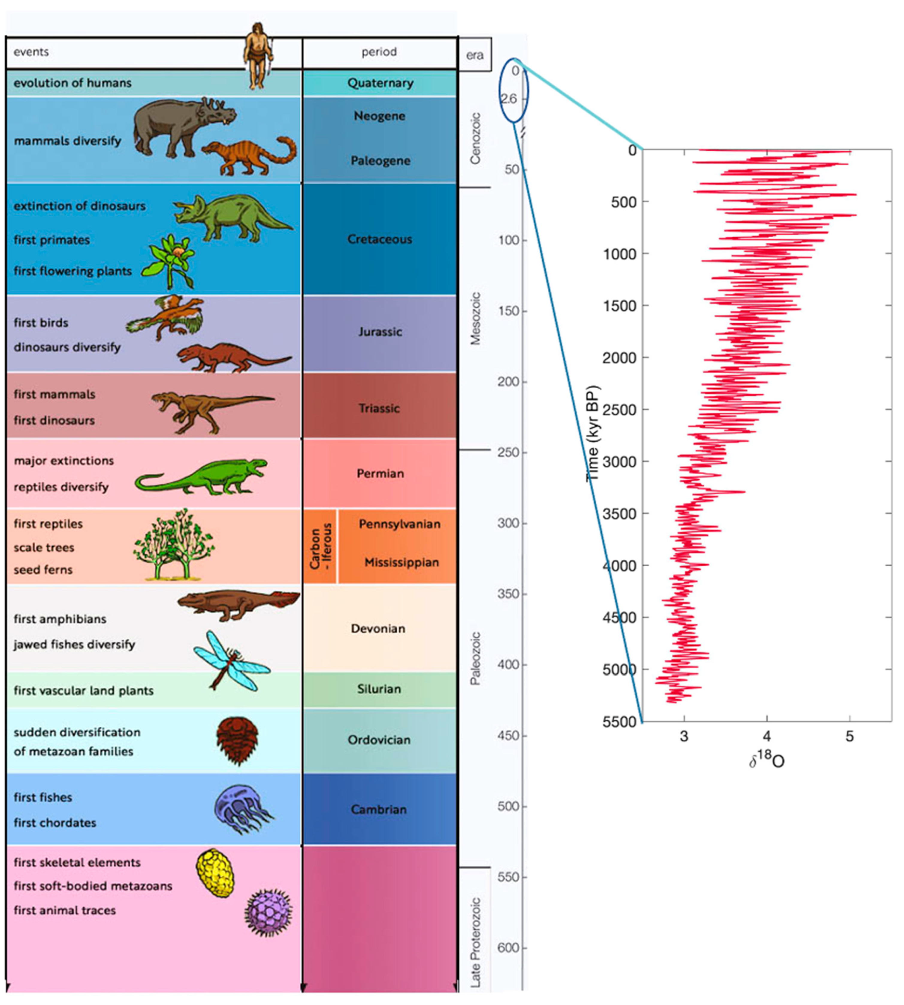
It is common knowledge that, at the Vostok scientific station, a group of Russian and French scientists investigated the East Antarctic ice extracting ice cores, which present layers produced by annual cycles of snow transformation into ice. In particular, in air bubbles trapped in layers of ice, isotopic oxygen ratios and gas composition measurements have allowed scientists to get information on the past planet temperature values [9,10,11,12,13]. In this framework, the Serbian astrophysicist Milutin Milankovitch studied the correlation between the Earth’s ice ages and the Earth’s movements. Milankovitch’s calculations, published in the 1920s, led him to conclude that there are three different cycles influencing the Earth’s climate. These are connected with the oscillations of the Earth’s orbit eccentricity, of the Earth’s axis and of the Earth’s axis wobble. The most recent Earth’s glacial age, within the Pleistocene, covered the time window from 2.6 million to 11,700 years before present (BP). The Vostok’s findings, which were later confirmed by other ice caps measurements, both in Antarctica and in Greenland, support the thesis that Milankovitch cycles pilot the glacial and interglacial temperature variations and that the latter are also connected to atmospheric greenhouse gas concentrations [14,15,16,17]. In particular, the Vostok station, located in the central part of East Antarctica, at an altitude of about 3500 m, shows an average annual temperature of T = −55 °C, with a lowest registered value in 1983 of T = −89.2 °C. Great care is necessary to not provoke ice coring fusion or contamination during the sample transport and to exclude misleading results arising from CO2 reactions with ice impurities [18,19,20]. More in details, the water molecules (H2O) containing O16, the most common O isotope, evaporate more than water molecules containing O18. Therefore, during the glacial age the ocean, water O18/O16 ratio rises, whereas in ice layers decreases, because O16-rich water evaporates from sea and is trapped in the glacier ice, whereas O18-rich water remains preferentially in the oceans [21,22,23,24,25]. By measuring the O18/O16 ratio, it is possible to obtain information on the past planet temperatures [26]. Figure 1 shows the geological scale and the scheme of life evolution on the planet during the last 630 M years BP (on the left) with a zoom on the last 5.5 M years BP that reports time behavior of the concentration as a function of time (on the right).
In the literature, different methods to investigate signal periodicities exist, with specific reference to the Fourier (FT) and to the wavelet (WT) transforms.
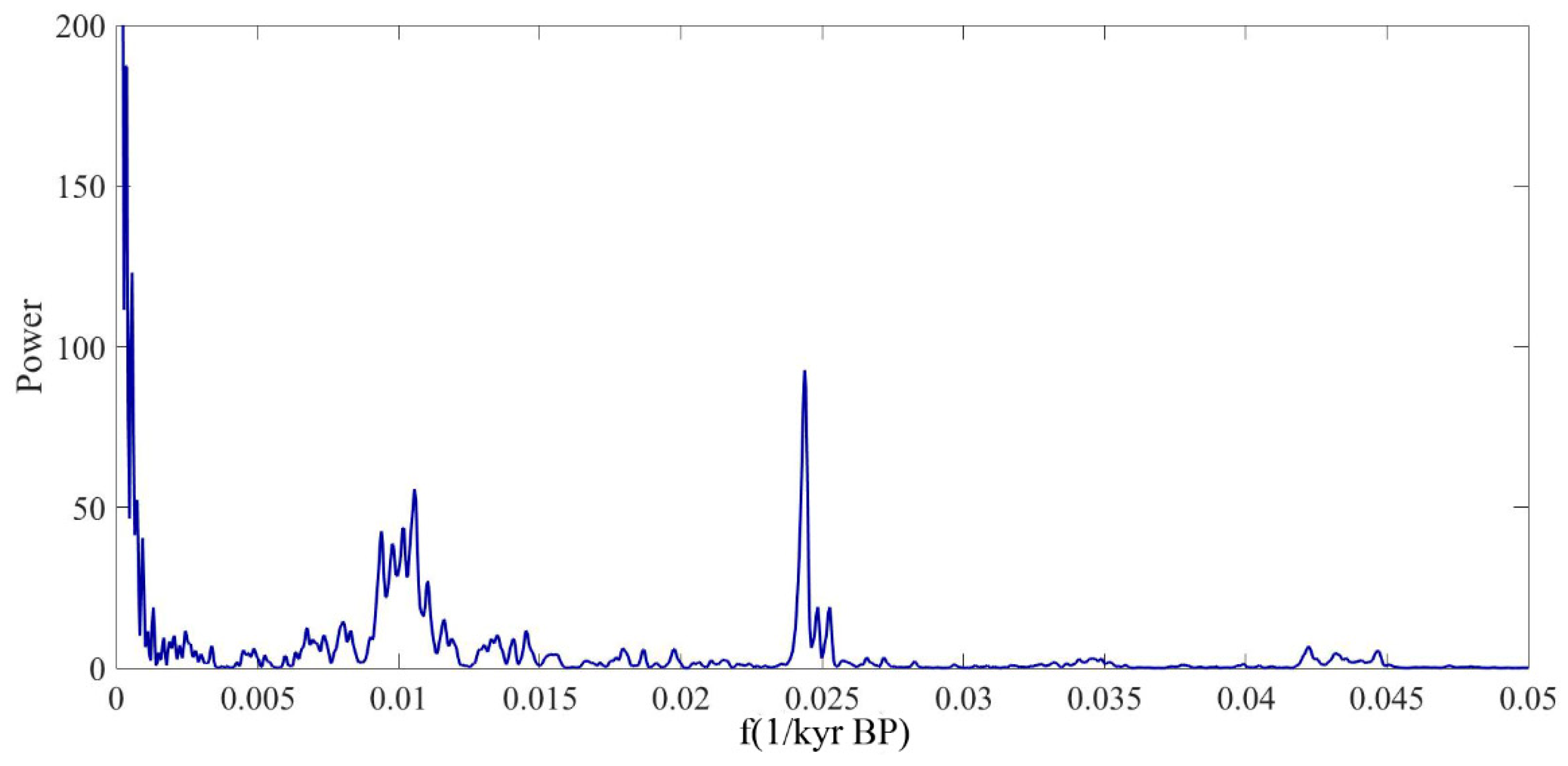
The calculated Fourier power spectrum of the not equispaced data record, performed by means of the Lomb–Scargle method [27,28,29,30], is shown in Figure 2. Such an analysis method allows researchers to detect periodic features in a series characterized by a not constant sampling.
In order to extract more information on the frequency components of the temperature variation as a function of time during the last 5.5 M years, in the following, we applied the wavelet analysis. It is well known that, when it is important to single out the signal frequency localizations, one can take a huge advantage from WT analysis [31,32,33,34,35,36]. In fact, differently from FT, which shows all the signal frequencies without a time localization, WT shows the component frequencies and at what time they occur [37,38,39].
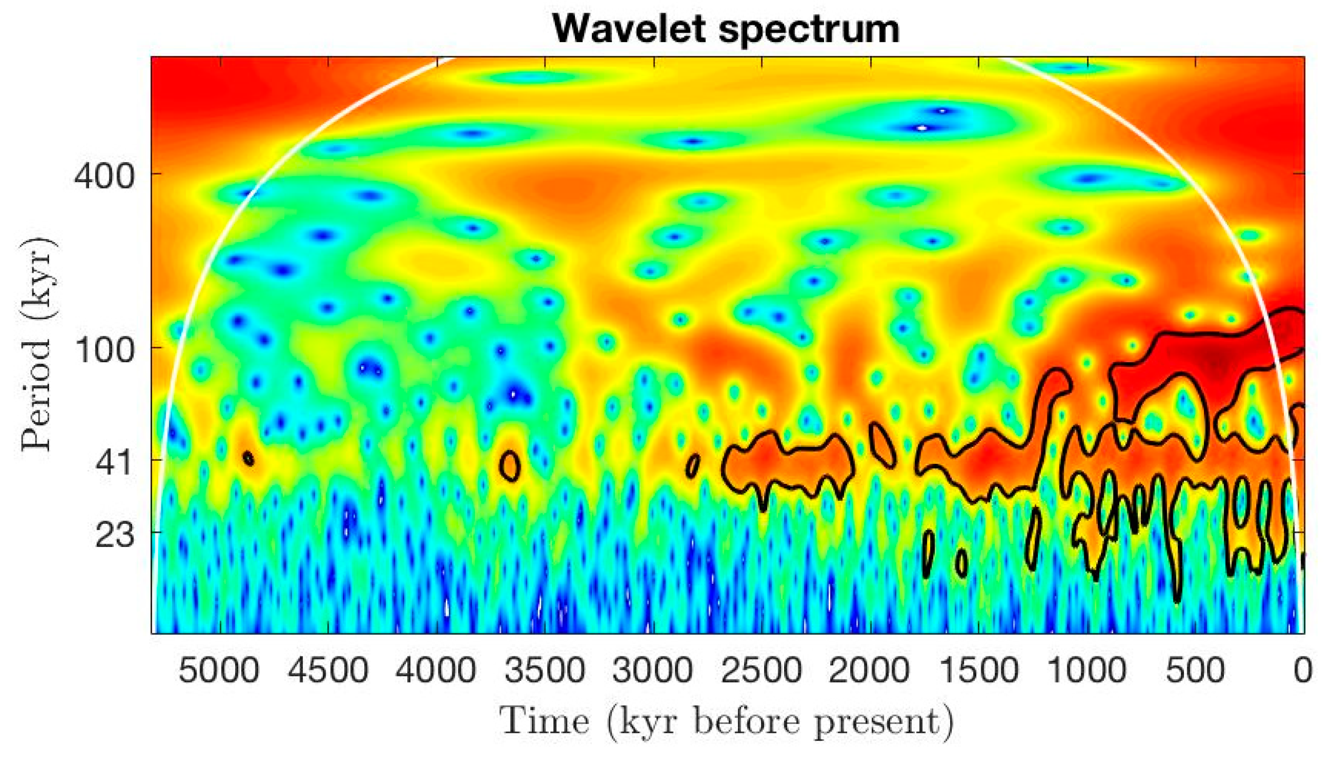
In Figure 3, the obtained WT scalogram of the temperature data, obtained by using an analytical Morlet wavelet with parameter 6 [40,41,42] is shown.
The performed WT analysis allowed us to draw the following conclusions:
- Variance increases, characterized by high ice volumes and by low temperature values, are present with a period of 100 K years; these maxima find a correspondence with the Earth’s orbit eccentricity period (first Milankovitch cycle);
- Variance increases are present in the temperature sequence with a period of 41 K years; these maxima correspond to the period of the Earth’s axis inclination (second Milankovitch cycle);
- Lower intensity variance increases with a period of about 23 K years, corresponding to the variation of the Earth’s axis during a double-conic motion, i.e., to solar precession, are present.
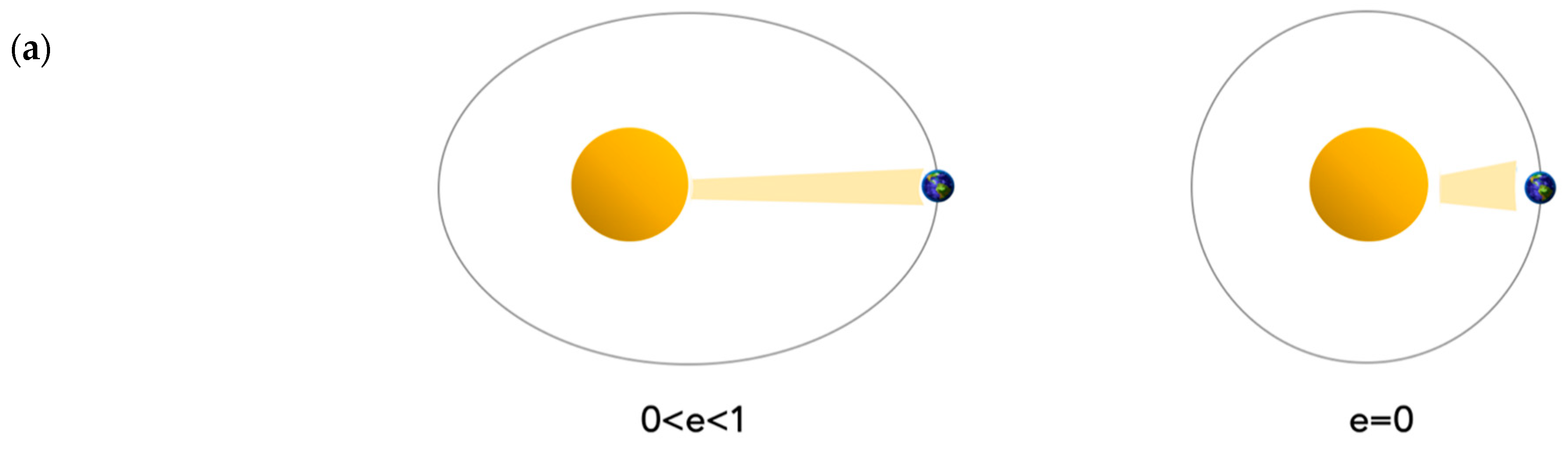
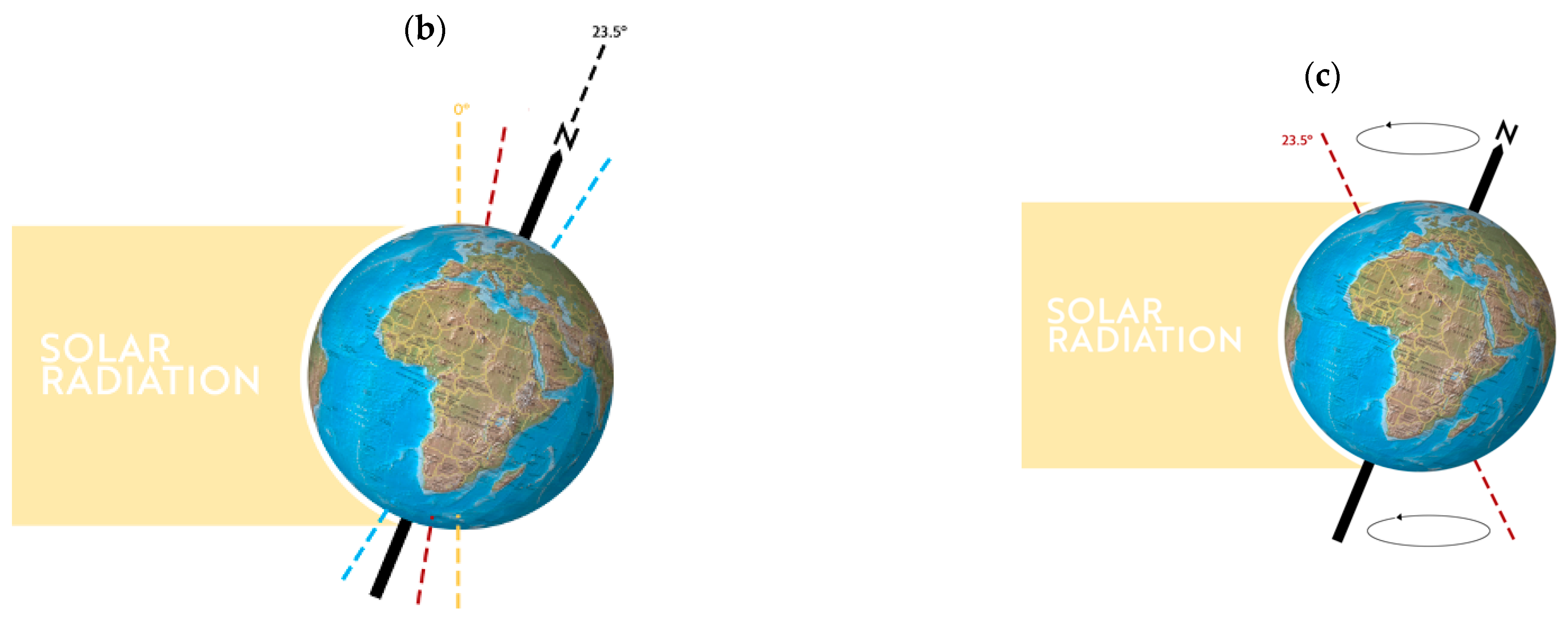
Furthermore, the obtained WT scalogram features are in good agreement with the prominent features reported by Crucifix [43]. Figure 4 shows a sketch of the three Milankovitch cycles. In particular, Figure 4a shows the Earth’s eccentricity variation characterized by a period of 100 K years. More specifically, the Earth’s orbit eccentricity has varied from nearly 0 to 0.07, and today its value is about 0.017. The Earth receives 20–30% more radiation when it is in the perihelion than when it is at aphelion. In particular, the average distance Sun–Earth is 1.49 1011 m, while the Sun’s average diameter is about 110 times that of the Earth (12.750 103 m). Figure 4b displays the cycle of the Earth’s axis inclination, ranging from a minimum of 21°55′ to a maximum of 24°20′, with a period of 41 K years. The inclination of the Earth’s axis relative to the orbit plane generates seasons. Slight changes in the tilt changes the amount of solar radiation falling on certain planet locations. The Earth’s axis is nowadays tilted of ~23.5 degrees, with a decreasing trend. Finally, Figure 4c shows the variation of the Earth’s axis following a double-cone motion, i.e., a precession motion, with a 23 K years period. This precession motion does not change the tilt of Earth’s axis, but its orientation. During the past millennia, the Earth’s axis pointed more or less north, towards Polaris, known as the Pole Star. However, about 5000 years ago the Earth was more turned towards another star, called Thubin. Moreover, in about 12,000 years, the axis will point to Vega. After a cycle of precession, the orientation of the planet is changed with respect to the aphelion and the perihelion: if a hemisphere is pointed towards the sun during the perihelion, it will be opposite during the aphelion, the vice versa being true for the other hemisphere. As a result, the hemisphere that is pointed towards the sun during perihelion and away during aphelion experiences more extreme seasonal contrasts than the other hemisphere. At present, winter in the southern hemisphere occurs near the aphelion and summer near the perihelion, which means that the southern hemisphere experiences more extreme seasons than the northern hemisphere [44,45,46,47,48,49].
As matter of fact, as shown by the cornerstone work of Benzi et al. [50], the variations in the distribution of solar radiation during Milankovitch cycles, alone, cannot explain the wide decrease in temperature that marks the transition from an interglacial age to a glacial age. Therefore, it clearly emerges that to enhance the effect of these causes, which foretell a temperature variation of only 0.3 K, a positive feedback should be taken into account. On that score, to figure out this puzzle, a stochastic resonance effect has been postulated. This effect concerns with nonlinear systems energetically characterized by a threshold (i.e., by an activation barrier), and consists of a system output (response) to a weak input signal (cause), which undergoes a resonance-like behavior, i.e., to a performance maximum, as a function of the noise level, differently to what occurs in linear systems where the output is maximized in the absence of noise [51,52,53]. In fact, the complex climate system contains several interacting components that give rise to a highly nonlinear behavior through its many feedback mechanisms.
Climatic driving mechanisms acting on human evolution constitute an open problem of interdisciplinary scientific interest that triggers an intense debate concerning possible evolutionary scenarios. The concentration increase of CO2 and other greenhouse gases in atmosphere influences the climate system significantly. The major role in determining the warming rate and its spatial distribution is played by ocean water, due to its heat capacity. On one hand, the climate response to temperature variation is delayed by the ocean; on the other hand, ocean water delays the warming effect on climate. Global surface temperatures show short and long time scales in the atmosphere–ocean general circulation, although fast and slow responses in the ocean are different from those in the atmosphere.
In this paper we addressed the issue of climate variability caused by internal processes, by external forcing, and by their interaction, and discuss mechanisms of a global Earth temperature increase. In particular, we explore the stochastic resonance scenario under the condition of a temperature increase, independently from peculiar, specific temperature trends. The results of the performed numerical simulations show that, starting from a resonance condition, an increase in temperature gives rise to a transition towards a chaotic regime.
2. Methods Section
It is well known that the Fourier approach is based on a definite set of sinusoidal functions, which provides a unique representation in terms of a standard orthogonal basis. Its weaknesses include the assumptions of linearity and stationarity and the a priori choice of basis functions, which do not change in time. This means that the projection of the basis results in a ‘global’ frequency analysis that may not provide a good match with the time scales of the underlying processes.
Some techniques have been designed to address the issue of nonstationarity, so as to provide a simultaneous time–frequency analysis. Two of such techniques are windowed Fourier analysis and wavelets. In windowed Fourier analysis, a Fourier analysis is applied to a sliding window, whose length is shorter than the given record; then, a projection is applied to each windowed subset of the data.
Wavelet analysis is based on a set of orthogonal functions with compact support or approximately compact support, vanishing outside a finite interval. The interval is rescaled to highlight different time scales and the center of interval can be shifted to address nonstationarity. The algorithm determining the decomposition coefficients is still a projection, but the resulting coefficients depend on the shape, the width, and location of interval of support. A set of orthonormal functions can be constructed from a “mother” wavelet via dilation and translation.
More specifically, from a formal point of view, a Fourier series decomposes a function
defined for
and having a period T =
into a sum of sinusoidal functions, i.e., of cosine and/or sine functions:
,
and
being the so-called Fourier coefficients, evaluated through the integrals:
where
furnishes the average value of the function f(t) over a period T =
and where the Fourier coefficients,
and
furnish the weight of each cosine and sine contributions; for odd functions all the
coefficients are zero whereas for even functions all the
coefficients are zero.
Fourier transform (FT) constitutes an extension of the Fourier series, which furnishes huge advantages for functions
that are nonperiodic, and therefore when
, FT decomposes the function f(t) into sets of sine and/or cosine functions, or of exponential functions
each of them with weight
with continuously variable frequencies
:
As a matter of fact, FT suffers from the limitation that it does not allow a connection between the frequency spectrum and the signal evolution in time and, therefore, to overcome this difficulty, wavelet (WT) analysis has been formulated [54,55,56].
WT results are more advantageous in respect to Fourier transform; in fact, the WT approach allows users to decompose a signal into its wavelets components, by means of mother wavelet
:
where the parameter
denotes the scale and its value corresponds to the inverse of the frequency, the parameter
represents the shift of the scaled wavelet along the time axis,
represents the complex conjugation of the mother wavelet, while the scaled and shifted mother wavelet
can be expressed by:
Differently from FT, which shows only which signal frequencies are present, WT, in addition, also shows where, or at what scale, they are. Furthermore, while FT allows researchers to decompose the signal only in cosine and sine component functions, the WT takes into account several wavelet mother functions.
More precisely, different types of mother wavelet can be used to perform a wavelet analysis. As a rule, mother wavelets are characterized by properties such as orthogonality, compact support, and symmetry. Although different mother wavelet functions satisfy the previous conditions, when applied to the same signal produce different results. For these reasons, the choice of the best mother wavelet is crucial. In the present study, a comparison among the different correlation degree between the signal and different mother wavelet functions has been performed [57]. As a result, in this work the wavelet Morlet has been chosen as mother wavelet:
where represents the center pseudo-frequency and provides the wavelet bandwidth [58,59]. It should be noticed that in the special case in which the wavelet mother is , the WT transform reduces to the FT. For this study, Matlab environment has been used.
3. The Physical Approach to Climate Change through the Stochastic Resonance Modelization
The stochastic resonance phenomenon takes place when the introduction of a noise in a nonlinear system characterized by a form of threshold amplifies a weak signal. In particular, it occurs that, by increasing the noise amplitude, the system performance parameters, e.g., the output signal-to-noise ratio (SNR), show a resonance. Therefore, such a behavior is different in respect to linear systems, where the SNR is maximized in the absence of noise.
The time evolution of the climate system configuration can be described by means of a configuration variable x(t), by means of a potential U(x) and of a random force through the Langevin equation:
where is a weak forcing term corresponding, within the climate model, to the 100,000-year Milankovitch cycle; is a white noise, of intensity , which corresponds to the fast dynamics and whose autocorrelation function is . In the following, we will assume that this latter hypothesis holds for the climate system. A simple example of potential is furnished by the symmetric bistable potential introduced by McNamara et al. [60]:
which has two stable equilibrium configurations at , and an unstable equilibrium configuration at ; the two stable minima correspond to the glacial and interglacial temperature states. In the absence of the forcing term, i.e., for , for assigned system parameters, the configuration variable fluctuates in time between the two minima with a variance that is proportional to , whereas in the presence of a periodic forcing term and of specific noise values, the transition probability of escaping from each well varies regularly in time. In particular, what emerges from the stochastic resonance modelling is that, for specific noise values, jumps between the two minima occur in synchrony with the frequency of the weak periodic signal.
4. Numerical Simulation of Climate Changes and Results
The climate system has a chaotic nature, where a very small perturbation can be amplified. This chaotic character is taken into account both explicitly, by introducing a noise term, or indirectly, by introducing small variations in the initial conditions or in some physical parameters; in this latter case, one usually copes with a huge number of runs for the same prevision and performs a probabilistic analysis [61,62,63,64,65,66]. In order to modelize the climate cycle behavior and the effects connected with the global temperature trend, in this section, we adapted the stochastic differential Langevin’s equation, which originally took into account only a systematic and a random contribution, to a dynamic case in which, besides a friction and a stochastic term, an external contribution and a double well potential were present [67,68,69,70,71]:
In other terms, the climate system is modelled as a particle of mass m, with a given average energy and configuration coordinate x(t), which experiences a force potential (x), and on which both a friction force, , i.e., a Stokes force, and a random force, , connected with the system “heat bath”, are exerted [72,73,74,75,76,77,78,79].
In the “high friction limit”, i.e., when the system’s acceleration is negligible, by including the constant
into the potential function
and into the random force
, Equation (11) becomes:
Let us now introduce an explicit form for a generalized potential conceived in order to include a simple double-well potential and a periodic contribution:
Under this hypothesis, Equation (12) can be written as:
where the quantities and allow researchers to describe with a greater detail the stochastic noise . Such a mathematical model allows users to describe the planet temperature behaviour when one identifies the Earth’s temperature [80,81]. is the Earth’s climate potential, which takes into account the energy balance between the incoming and outcoming radiation and the two system levels describing the glacial (T1 ≅ 278.6 K) and interglacial (T2 ≅ 283.3 K) states [82,83,84]. In particular, it is: , where is the solar constant and A is the amplitude of the modulation, estimated, by Milankovitch, to be equal to 5 × 10⁻⁴, with . Furthermore, , where is the albedo, i.e., the reflected solar radiation which, for simplicity, has a linear decreasing trend with temperature, and is the energy radiated by the Earth according to its temperature T. Then, it is (c being the Earth’s thermal capacity). Finally, the stochastic noise represents the short time scale processes connected with atmospheric dynamics and circulation. In short, in terms of temperatures value, we have:
As shown by Benzi et al. [85], depending on the values, in spite of the weakness of the periodic contribution , which in our modelization corresponded to the first Milankovitch cycle, it is possible to get an amplification of the signal, so justifying the remarkable gap of almost 10 °C between glacial and interglacial periods.
In the present work, with the aim to single out the effects of temperature increase on the above described SR scenario, at first we performed numerical simulations on a system characterized by a double-well potential, which allowed us to describe the glacial and interglacial states. In the model drawing up, we have taken into account a small periodic disturbance, , which allowed us to describe the Earth’s orbit eccentricity cycle, and a noise level of amplitude fixed on the SR condition.
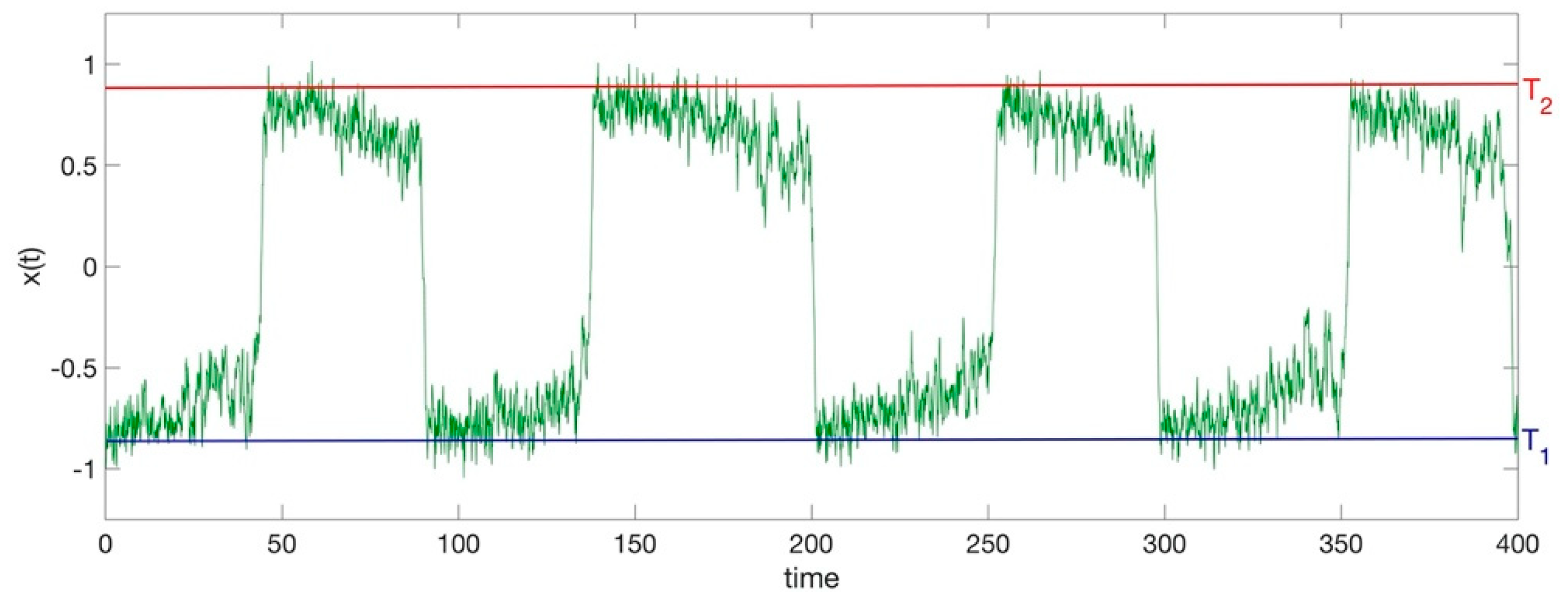
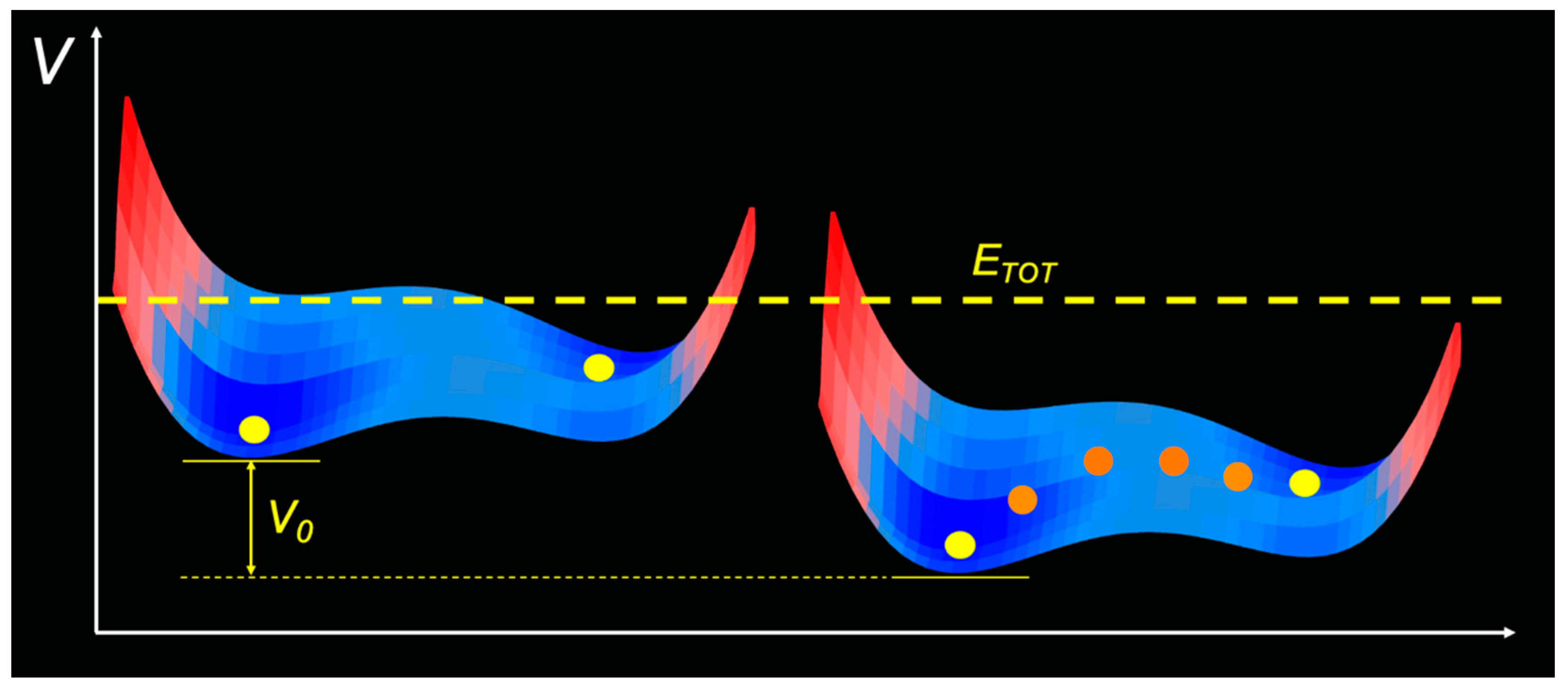
In this framework, starting from the obtained resonance conditions, we have performed new numerical simulations, taking into account increasing global Earth temperature values. This temperature increase has been taken into account by downshifting the double-well potential of a constant term with respect to the fixed total energy of the system, i.e., in such a case, in fact, although the driving force keeps constant, see Equation (15), the downshift of the potential well, keeping constant the total energy, corresponds to an increase of the system kinetic energy, and hence of temperature. In other words, the simulations have been performed at first by varying the intensity of the noise while keeping the periodic signal constant in order to single out the noise amplitude value, for which the jump of the system from one hole to the other one is synchronized with the external system periodic disturbance; in such a way, the resonance condition was obtained [86,87]. Successively, starting from this SR condition, we have simulated the modelled system answer for different values of the global planet temperature. Figure 5 reports the solution of Equation (14), i.e., the x(t) = T(t), by using the following parameters: = 0.46 and . As it can be seen, under such a situation, the system jumped from the left well to the right well, giving rise to a periodic oscillation between the two wells corresponding to the glacial (at temperature T1) and interglacial (at temperature T2) states [88,89,90].
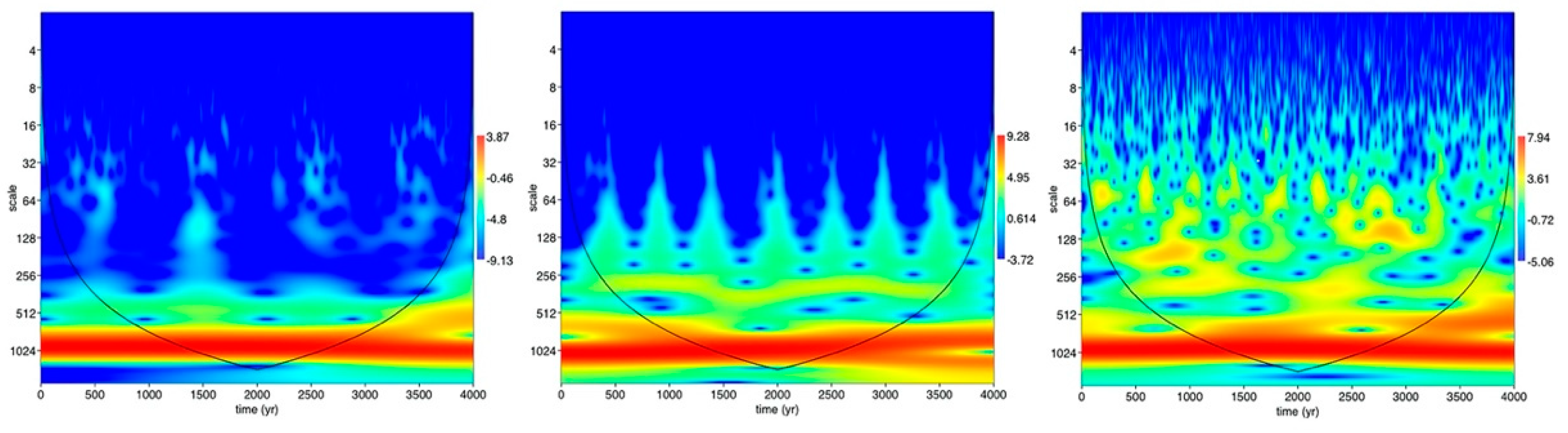
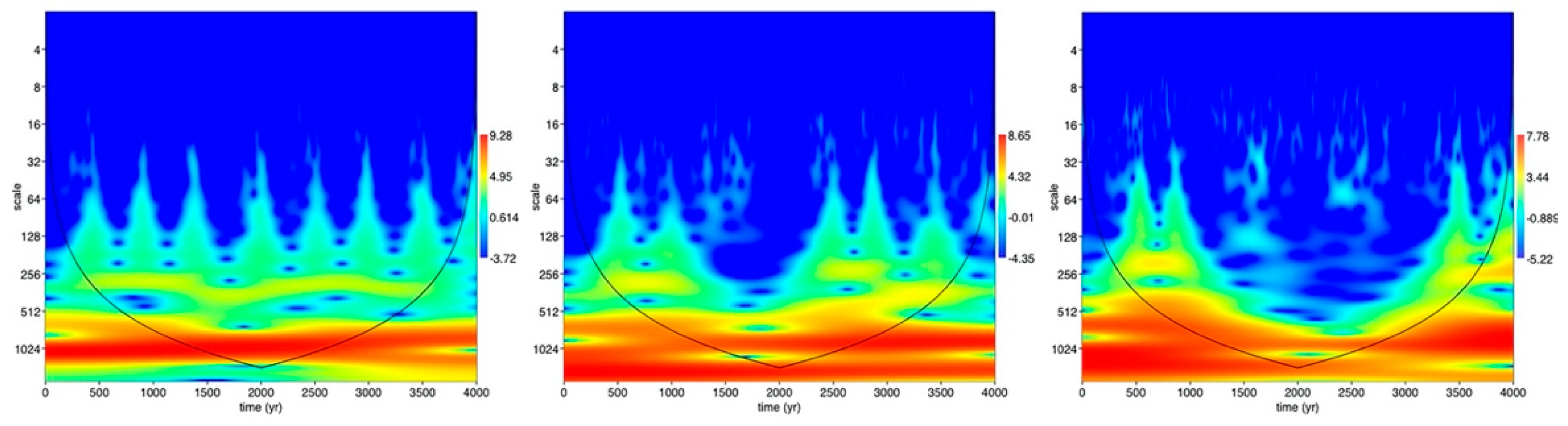
To spotlight the SR condition and to quantitatively determine the signal-to-noise ratio, SNR, a WT scalogram of the obtained solution, i.e., x(t) = T(t), has been evaluated for the fixed value of a = 0.46 and for different values of α, i.e., α = 0.05 (left side), 0.23 (center), and 0.70 (right side), as reported in Figure 6.
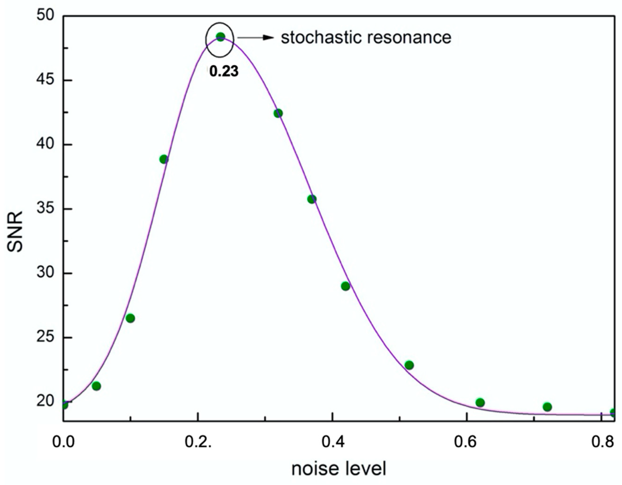
Such a WT approach allowed us to evaluate the SNR value, for different noise levels [91,92,93,94,95]. The result of such a calculation for 12 values of noise, in the range 0.000.83, is shown in Figure 7. These results put in the foreground that, starting from low noise levels, at first, the SNR value surged, attaining a maximum of a = 0.46 and α = 0.23 and then it dropped for higher noise values. Therefore, for a = 0.46, the value of α = 0.23 established a cutting-edge between increasing and decreasing SNR conditions [96,97,98,99,100,101].
During the last few decades, there has been considerable progress in understanding climate variability by large observational efforts, model simulations, and theory development. In the next section, following the proposed SR climate model, we present the results of new numerical simulations that will show how, starting from a resonance condition, an increase of temperature gives rise to transition to a chaotic regime.
5. Effects of the Global Climate Warming on the Basis of the SR Climate Model
A climate change is considered anomalous when it is not compatible with only its internal variability within a period of time longer than about 30 years. The evidence of a global climate change is based on the analysis of the long-term variability that affects the different components of the climate system, which are the atmosphere (i.e., the shell of gases and vapors around the Earth), the hydrosphere (i.e., seas, rivers, water basins), the cryosphere (i.e., sea ices, snows, glaciers, iced soils), the biosphere (i.e., the living organisms), and the lithosphere (i.e., Earth’s crust). These elements continuously exchange energy and matter (i.e., water, mineral and/or organic substances) between each other; furthermore, their interactions are modulated by planet radiative balance fluctuations, which can be amplified or stabilized by positive or negative feedback physical processes (positive and negative retroactions). Atmosphere constitutes the rapid component of the climate system, since the air masses mix, at the planetary level, within some months, whereas the seas interact with the atmosphere from both short time scales (i.e., daily) through to several decades. Sea currents are due to the Earth’s rotation, winds, and seas density, which in turn depends on sea temperature and salinity. Climate changes depend on external forcing, i.e., perturbations external to the climate systems (e.g., orbital parameters, variations of Sun’s activity), or by internal forcing (e.g., El Nino). Furthermore, anthropic activities produce greenhouse gases, such as carbon dioxide (CO2), methane (CH4), nitrogen protoxyde (N2O), etc.; aerosols (small solid or liquid particles); and changes in the soil usage (e.g., deforestation, agriculture).
The climate trend can be inferred from the analysis of long-term datasets, which are essentially based on paleoclimate archives of different climate-dependent chemical–physical quantities, often integrated through numerical and interpretative models. In fact, climate changes leave indirect information in the physical, chemical, and biological compositions of natural materials, i.e., in proxy data. In particular, the observations and the available measurements of the atmosphere, of the oceans, and of the Earth’s surface parameters indicate unequivocally that since the nineteenth century, the planet has started to undergo to a warming process. In recent decades, soil and ocean temperatures, on average, have increased, even if not homogeneously, but with greater warming near polar latitudes, especially in the Arctic region.
In the meantime, the ice and snow coverage has decreased in different areas of the planet. The atmospheric water vapor content has increased everywhere due to the higher temperature of the atmosphere, while sea level has also risen. Furthermore, changes in several other climatic indicators have also been detected; these include the seasonal extension in many places of the planet; an increase in the tendency of extreme meteorological events, such as heat waves or heavy rainfall; and a general decrease in extreme cold events. As far as the cause of the registered warming is concerned, if one takes into account only the natural forcing, it is not possible to justify these climatic changes. Most of the warming effects observed globally over the last 50 years can only be explained if one takes into account the effects produced by human activities, and in particular both the emissions from fossil fuels and the deforestation processes [102,103,104,105].
The series of global temperatures registered over the period 1840–2017 show a warming trend interrupted only for short periods. In particular, the decade between 1900 and 1910 and that between 1942 and 1950 represent the only time intervals in which global temperatures have undergone a reversal trend. Moreover, starting from the late 1970s, the slope of the regression line has undergone a substantial increase, which has brought the heating values between 1970 and 2017 to about 0.17 °C/decade [106,107,108,109,110,111].
In this framework, with the aim to single out the effects of temperature increase on the above described SR scenario, starting from the resonance condition obtained at = 0.46 for , we next focused our attention on the SR model outcomes for increasing values of the Earth’s temperature. More specifically, to cope with the effects of global warming within the SR scenario, we performed new numerical simulations for a sequence of downshifted double-well potentials (see Figure 8).
In fact, a temperature increase corresponded to a downshift of the system potential energy, furnishing a dummy run of the system behaviour. As an example, Figure 9 shows three WT scalograms of the generalized Langevin’s equation solution for , , and . As it can be seen, the Earth’s temperature increase gave rise to a breaking of the stochastic resonance condition.
In summary, in this study we have tested the climate stochastic resonance model under the condition of a temperature increase. More specifically, within this framework model, we have determined the resonance stochastic condition by varying at first the noise level and by applying the wavelet analysis; then, once the resonance condition has been reached, by keeping constant the noise level, new simulations were performed by varying the thermal potential. As a result, the simulation results indicate a transition towards a chaotic regime, where the Milankovitch cycle effects disappear.
6. Conclusions
The last few decades have registered the hottest temperature variation in recorded history. In this framework, the effects provided by a global temperature increase on climate behavior, as inferred by both applying the stochastic resonance interpretative model for climate and WT data analysis, are discussed.
In particular, a Milankovitch-cycle-breaking scenario induced by a triggering temperature increase, independently from a peculiar temperature trend, is forecasted by the climate stochastic resonance model. Numerical simulations for increasing planet temperatures have been performed. The simulations’ outcomes beget the following scenario: starting from the resonance condition, the Earth’s temperature increase boosts a transition towards a chaotic regime, where the Milankovitch cycles disappear. It should be noticed that, although meteorology and climate drastically differ for the involved time scales, they constitute the two faces of the same coin. In this framework, the obtained results justify, on short time scales, the registered intensity increase of extreme meteorological events. If the greenhouse gas emissions continue to increase at the present rate during the XXI century, a temperature increase of 5 ± 1 °C is expected by the year 2100 in respect to the value corresponding to the beginning of the industrial era; this would also imply a rise of the sea level of 75 ± 20 cm. For these reasons, as well as in consideration of the climate system high inertia connected to the residence time of CO2 in the atmosphere, it is important to stabilize the global temperature within +2 °C by 2100 compared to the preindustrial value, in agreement to the international treatises.
Author Contributions
M.T.C. and S.M. contributed equally; in particular M.T.C. and S.M. performed theoretical and numerical analysis, contributed analytic tools and interpreted the data, wrote the main draft of the paper, and participated in revising the manuscript. All authors have read and agreed to the published version of the manuscript.
Funding
This research received no external funding.
Conflicts of Interest
The authors declare no conflict of interest.
References
- Jacka, T.H.; Budd, W.F. Detection of temperature and sea-ice-extent changes in the Antarctic and Southern Ocean, 1949–1996. Ann. Glaciol. 1998, 27, 553–559. [Google Scholar] [CrossRef] [Green Version]
- Caccamo, M.T.; Castorina, G.; Colombo, F.; Insinga, V.; Maiorana, E.; Magazù, S. Weather forecast performances for complex orographic areas: Impact of different grid resolutions and of geographic data on heavy rainfall event simulations in Sicily. Atmos. Res. 2017, 198, 22–33. [Google Scholar] [CrossRef]
- Jones, P.D. Recent variations in mean temperature and the diurnal temperature range in the Antarctic. Geophys. Res. 1995, 22, 1345–1348. [Google Scholar] [CrossRef]
- Raper, S.C.; Wigley, T.M.; Jones, P.D.; Salinger, M.J. Variations in surface air temperatures: Part 3. The Antarctic, 1957–1982. Mon. Weather Rev. 1984, 112, 1341–1353. [Google Scholar] [CrossRef] [Green Version]
- Monnin, E.; Indermuhle, A.; Dallenbach, A.; Fluckiger, J.; Stauffer, B.; Stocker, T.F.; Raynaud, D.; Barnola, J.-M. Atmospheric CO2 Concentrations over the Last Glacial Termination. Science 2001, 291, 112–114. [Google Scholar] [CrossRef] [Green Version]
- Nakamura, K.; Doi, K.; Shibuya, K. Estimation of seasonal changes in the flow of Shirase Glacier using JERS-1/SAR image correlation. Polar Sci. 1984, 1, 73–84. [Google Scholar] [CrossRef] [Green Version]
- Davey, M.C. Effects of continuous and repeated dehydration on carbon fixation by bryophytes from the maritime Antarctic. Oecologia 1997, 110, 25–31. [Google Scholar] [CrossRef]
- Caccamo, M.T.; Magazù, S. A Physical–Mathematical Approach to Climate Change Effects through Stochastic Resonance. Climate 2019, 7, 21. [Google Scholar] [CrossRef] [Green Version]
- Barnola, J.M.; Raynaud, D.; Korotkevich, Y.S.; Lorius, C. Vostok ice core provides 160,000-year record of atmospheric CO2. Nature 1987, 329, 408–414. [Google Scholar] [CrossRef]
- Jouzel, J.; Lorius, C.; Petit, J.R.; Genthon, C.; Barkov, N.I.; Kotlyakov, V.M.; Petrov, V.M. Vostok ice core: A continuous isotopic temperature record over the last climatic cycle (160,000 years). Nature 1987, 329, 403–408. [Google Scholar] [CrossRef]
- Pepin, L.; Raynaud, D.; Barnola, J.M.; Loutre, M.F. Hemispheric roles of climate forcings during glacial-interglacial transitions as deduced from the Vostok record and LLN-2D model experiments. J. Geophys. Res. 2001, 106, 31885–31892. [Google Scholar] [CrossRef]
- Petit, J.R.; Basile, I.; Leruyuet, A.; Raynaud, D.; Lorius, C.; Jouzel, J.; Stievenard, M.; Lipenkov, V.Y.; Barkov, N.I.; Kudryashov, B.B.; et al. Four climate cycles in Vostok ice core. Nature 1997, 387, 359–360. [Google Scholar] [CrossRef] [Green Version]
- von der Heydt, A.; Ashwin, S.P.; Camp, C.D.; Crucifix, M.; Dijkstra, H.A.; Ditlevsen, P.; Lenton, T.M. Quantification and interpretation of the climate variability record. Glob. Planet. Chang. 2021, 197, 103399. [Google Scholar] [CrossRef]
- Liu, H.S. A new view on the driving mechanism of Milankovitch glaciation cycles. Earth Plan. Sci. Lett. 1995, 131, 17–26. [Google Scholar] [CrossRef]
- Becker, J.; Lourens, L.J.; Hilgen, F.J.; Van Der Laan, E.; Kouwenhoven, T.J.; Reichart, G.-J. Late Pliocene climate variability on Milankovitch to millennial time scales: A high-resolution study of MIS100 from the Mediterranean. Palaeogeogr. Palaeoclim. Palaeoecol. 2005, 228, 338–360. [Google Scholar] [CrossRef]
- Lachniet, M.; Asmerom, Y.; Polyak, V.; Denniston, R. Arctic cryosphere and Milankovitch forcing of Great Basin paleoclimate. Sci. Rep. 2017, 7, 12955. [Google Scholar] [CrossRef] [PubMed] [Green Version]
- Petit, J.R.; Jouzel, J.; Raynaud, D.; Barkov, N.I.; Barnola, J.-M.; Basile-Doelsch, I.; Bender, M.L.; Chappellaz, J.; Davis, M.L.; Delaygue, G.; et al. Climate and atmospheric history of the past 420,000 years from the Vostok ice core, Antarctica. Nature 1999, 399, 429–443. [Google Scholar] [CrossRef] [Green Version]
- Basile, I.; Grousset, F.E.; Revel, M.; Petit, J.R.; Biscalye, P.E.; Barkov, N.I. Patagonian origin dust deposited in East Antarctica (Vostok and Dome C) during glacial stages 2, 4 and 6. Earth Planet. Sci. Lett. 1997, 146, 573–589. [Google Scholar] [CrossRef]
- Waelbroeck, C.; Jouzel, J.; Labeyrie, L.; Lorius, C.; Labracherie, M.; Stiévenard, M.; Barkov, N.I. A comparison of the Vostok ice deuterium record and series from Southern Ocean core MD 88-770 over the last two glacial-interglacial cycles. Clim. Dyn. 1995, 12, 113–123. [Google Scholar] [CrossRef]
- Suwa, M.; Bender, M.L. Chronology of the Vostok ice core constrained by O2/N2 ratios of occluded air, and its implication for the Vostok climate records. Quat. Sci. Rev. 2008, 27, 1093–1106. [Google Scholar] [CrossRef]
- Landais, A.; Barkan, E.; Luz, B. Record of delta δ18O and 17O-excess in ice from Vostok Antarctica during the last 150,000 years. Geophys. Res. Lett. 2008, 35, L02709. [Google Scholar]
- Bopp, L.; Kohfeld, K.E.; Le Quere, C.; Aumont, O. Dust impact on marine biota and atmospheric CO2 during glacial periods. Paleoceanography 2003, 18, 1046. [Google Scholar] [CrossRef]
- Farquhar, G.D.; Lloyd, J.; Taylor, J.A.; Flanagan, L.B.; Syvertsen, J.P.; Hubick, K.T.; Wong, S.C.; Ethleringer, J.R. Vegetation effects on the isotope composition of oxygen in atmospheric CO2. Nature 1993, 363, 439–442. [Google Scholar] [CrossRef]
- Bargagli, R.; Agnorelli, C.; Borghini, F.; Monaci, F. Enhanced deposition and bioaccumulation of mercury in Antarctic terrestrial ecosystems facing a coastal polynya. Environ. Sci. Technol. 2005, 39, 8150–8155. [Google Scholar] [CrossRef] [PubMed]
- Richardson, A.J.; Schoeman, D.S. Climate impact on ecosystems in the northeast Atlantic. Science 2004, 305, 1609–1612. [Google Scholar] [CrossRef]
- Lisiecki, L.E.; Raymo, M.E. A Pliocene-Pleistocene stack of 57 globally distributed benthic δ18O records. Paleoceanography 2005, 20, 1003. [Google Scholar] [CrossRef] [Green Version]
- Ruf, T. The Lomb-Scargle Periodogram in Biological Rhythm Research: Analysis of Incomplete and Unequally Spaced Time-Series. Biol. Rhythm Res. 1999, 30, 178–201. [Google Scholar] [CrossRef]
- Van Dongen, H.P.A.; Olofsen, E.; Van Hartevelt, J.H.; Kruyt, E.W. A Procedure of Multiple Period Searching in Unequally Spaced Time-Series with the Lomb–Scargle Method. Biol. Rhythm Res. 1999, 30, 149–177. [Google Scholar] [CrossRef]
- Pardo-Igúzquiza, E.; Rodríguez-Tovar, F.J. Spectral and cross-spectral analysis of uneven time series with the smoothed Lomb–Scargle periodogram and Monte Carlo evaluation of statistical significance. Comput. Geosci. 2012, 49, 207–216. [Google Scholar] [CrossRef]
- Glynn, E.F.; Chen, J.; Mushegian, A.R. Detecting periodic patterns in unevenly spaced gene expression time series using Lomb–Scargle periodograms. Bioinformatics 2006, 22, 310–316. [Google Scholar] [CrossRef] [PubMed] [Green Version]
- Priestley, M.B. Spectral Analysis and Time Series. J. Time Ser. Anal. 1996, 17, 85–103. [Google Scholar] [CrossRef]
- Caccamo, M.T.; Magazù, S. Variable mass pendulum behaviour processed by wavelet analysis. Eur. J. Phys. 2017, 38, 15804. [Google Scholar] [CrossRef]
- Caccamo, M.T.; Cannuli, A.; Magazù, S. Wavelet analysis of near-resonant series RLC circuit with time-dependent forcing frequency. Eur. J. Phys. 2018, 39, aaae77. [Google Scholar] [CrossRef]
- Caccamo, M.T.; Magazù, S. Variable length pendulum analyzed by a comparative Fourier and wavelet approach. Rev. Mex. Fisica E 2018, 64, 81–86. [Google Scholar]
- Rioul, O.; Vetterli, M. Wavelets and Signal Processing. Signal Process. Mag. 1991, 8, 14–38. [Google Scholar] [CrossRef] [Green Version]
- Prokoph, A.; Patterson, R.T. Application of wavelet and discontinuity analysis to trace temperature changes: Eastern Ontario as a case study. Atmos. Ocean 2004, 42, 201–212. [Google Scholar] [CrossRef]
- Mallat, S.G. A theory for multiresolution signal decomposition: The wavelet representation. IEEE Trans. Pattern Anal. 1989, 11, 674–693. [Google Scholar] [CrossRef] [Green Version]
- Daubechies, I. The wavelet transform, time-frequency localization and signal analysis. IEEE Trans. Inform. Theory 1990, 36, 961–1005. [Google Scholar] [CrossRef] [Green Version]
- Blinowska, K.J.; Durka, P.J. Introduction to wavelet analysis. Br. J. Audiol. 1997, 31, 449–459. [Google Scholar] [CrossRef] [PubMed]
- Galli, A.W.; Heydt, G.T.; Ribeiro, P.F. Exploring the power of wavelet analysis. IEEE Comput. Appl. Power 1996, 9, 37–41. [Google Scholar] [CrossRef]
- Morlet, J.; Arens, G.; Fourgeau, E.; Glard, D. Wave propagation and sampling theory; Part I, Complex signal and scattering in multilayered media. Geophysics 1982, 47, 203–221. [Google Scholar] [CrossRef] [Green Version]
- Kronland-Martinet, R.; Morlet, J.; Grossmann, A. Analysis of sound patterns through wavelet transform. Int. J. Pattern Recognit. 1987, 1, 97–126. [Google Scholar] [CrossRef]
- Crucifix, M. Oscillators and relaxation phenomena in Pleistocene climate theory. Philos. Trans. R. Soc. A 2012, 370, 1140–1165. [Google Scholar] [CrossRef] [PubMed] [Green Version]
- Lisiecki, L. Links between eccentricity forcing and the 100,000-year glacial cycle. Nat. Geosci. 2010, 3, 349–352. [Google Scholar] [CrossRef]
- Williams, D.R.; Kasting, J.F. Habitable Planets with High Obliquities. Icarus 1997, 129, 254–267. [Google Scholar] [CrossRef]
- Gardner, G. Quantity of heat energy received from the sun. Sol. Energy 1960, 4, 26–28. [Google Scholar] [CrossRef]
- Bertolucci, S.; Zioutas, K.; Hofmann, S.; Maroudas, M. The Sun and its Planets as detectors for invisible matter. Phys. Dark Universe 2017, 17, 13–21. [Google Scholar] [CrossRef]
- Rolf, T.; Pesonen, L.J. Geodynamically consistent inferences on the uniform sampling of Earth’s paleomagnetic inclinations. Gondwana Res. 2018, 63, 1–14. [Google Scholar] [CrossRef]
- Fu, B.; Sperber, E.; Eke, F. Solar sail technology—A state of the art review. Prog. Aerosp. Sci. 2016, 86, 1–19. [Google Scholar] [CrossRef]
- Benzi, R.; Parisi, G.; Sutera, A.; Vulpiani, A. Stochastic resonance in climatic change. Tellus 1982, 34, 10–16. [Google Scholar] [CrossRef]
- Gang, H.; Gong, D.-C.; Wen, X.-D.; Yang, C.-Y.; Qing, G.-R.; Li, R. Stochastic resonance in a nonlinear system driven by an aperiodic force. Phys. Rev. A 1992, 46, 3250–3254. [Google Scholar] [CrossRef]
- Fauve, S.; Heslot, F. Stochastic resonance in a bistable system. Phys. Lett. A 1983, 97, 5–7. [Google Scholar] [CrossRef]
- Nicolis, C. Stochastic resonance in multistable systems: The role of intermediate states. Phys. Rev. E 2010, 82, 011139. [Google Scholar] [CrossRef] [PubMed]
- Bracewell, R.N. The Fourier Transform and Its Applications, 3rd ed.; McGraw-Hill: New York, NY, USA, 1999; pp. 84–102. [Google Scholar]
- Carslaw, H.S. Introduction to the Theory of Fourier’s Series and Integrals and the Mathematical Theory of the Conduction of Heat; MacMillan & Co.: London, UK, 1906; pp. 55–79. [Google Scholar]
- Eagle, A. A Practical Treatise on Fourier’s Theorem and Harmonic Analysis for Physicists and Engineers; Longmans, Green and Co.: New York, NY, USA, 1925; pp. 65–84. [Google Scholar]
- Ngui, W.K.; Leong, M.S.; Hee, L.M.; Abdelrhman, A.M. Wavelet analysis: Mother wavelet selection methods. Appl. Mech. Mater. 2013, 393, 953–958. [Google Scholar] [CrossRef]
- Astafeva, N.M. Wavelet analysis: Basic theory and some applications. Phys. Uspekhi 1996, 39, 1085–1108. [Google Scholar] [CrossRef]
- Bachman, G.; Narici, L.; Beckenstein, E. Fourier and Wavelet Analysis; Springer: Berlin/Heidelberg, Germany, 2000; pp. 263–388. [Google Scholar]
- McNamara, B.; Wiesenfeld, K. Theory of stochastic resonance. Phys. Rev. A 1989, 39, 4854–4869. [Google Scholar] [CrossRef] [PubMed]
- Benzi, R.; Sutera, A.; Vulpiani, A. The mechanism of stochastic resonance. J. Phys. A 1981, 14, 453–457. [Google Scholar] [CrossRef]
- Gammaitoni, L.; Bulsara, A.R. Nonlinear sensors activated by noise. Physica A 2003, 325, 152–164. [Google Scholar] [CrossRef]
- Benzi, R. Stochastic resonance: From climate to biology. Nonlinear Process. Geophys. 2010, 17, 431–441. [Google Scholar] [CrossRef]
- Kohar, V.; Murali, K.; Sinha, S. Enhanced Logical Stochastic Resonance under Periodic Forcing. Commun. Nonlinear Sci. 2014, 19, 2866–2873. [Google Scholar] [CrossRef]
- Parrondo, J.M.R.; De Cisneros, B.J. Energetics of Brownian motors: A review. Appl. Phys. A 2002, 75, 179–191. [Google Scholar] [CrossRef]
- Lai, Z.H.; Liu, J.S.; Zhang, H.T.; Zhang, C.L.; Zhang, J.W.; Duan, D.Z. Multi-parameter-adjusting stochastic resonance in a standard tri-stable system and its application in incipient fault diagnosis. Nonlinear Dyn. 2019, 96, 2069–2085. [Google Scholar] [CrossRef]
- Bulsara, A.R.; Dari, A.; Ditto, W.L.; Murali, K.; Sinha, S. Logical stochastic resonance. Chem. Phys. 2010, 375, 424–434. [Google Scholar] [CrossRef]
- Shi, P.; An, S.; Li, P.; Han, D. Signal feature extraction based on cascaded multistable stochastic resonance denoising and EMD method. Measurement 2016, 90, 318–328. [Google Scholar] [CrossRef]
- Schiavoni, M.; Carminati, F.R.; Sanchez-Palencia, L.; Renzoni, F.; Grynberg, G. Stochastic resonance in periodic potentials: Realization in a dissipative optical lattice. EPL 2002, 59, 493–500. [Google Scholar] [CrossRef] [Green Version]
- McDonnell, M.D.; Abbott, D. What is stochastic resonance? Misconceptions, Debates and its relevance to Biology. PLoS Comput. Biol. 2009, 5, e1000348. [Google Scholar] [CrossRef] [PubMed] [Green Version]
- Gammaitoni, L.; Hänggi, P.; Jung, P.; Marchesoni, F. Stochastic resonance. Rev. Mod. Phys. 1998, 70, 223–287. [Google Scholar] [CrossRef]
- Hänggi, P.; Inchiosa, M.E.; Fogliatti, D.; Bulsara, A.R. Nonlinear stochastic resonance: The saga of anomalous output-input gain. Phys. Rev. E 2000, 62, 6155–6163. [Google Scholar] [CrossRef] [PubMed] [Green Version]
- Gammaitoni, L.; Hänggi, P.; Jung, P.; Marchesoni, F. Stochastic resonance: A remarkable idea that changed our perception of noise. Eur. Phys. J. B 2009, 69, 1–3. [Google Scholar] [CrossRef]
- Wellens, T.; Shatokhin, V.; Buchleitner, A. Stochastic resonance. Rep. Prog. Phys. 2004, 67, 45–105. [Google Scholar] [CrossRef]
- Berdichevsky, V.; Gitterman, M. Stochastic resonance in linear systems subject to multiplicative and additive noise. Phys. Rev. E 1999, 60, 1494–1499. [Google Scholar] [CrossRef] [PubMed]
- Li, J.H.; Han, Y.X. Phenomenon of stochastic resonance caused by multiplicative asymmetric dichotomous noise. Phys. Rev. E 2006, 74, 051115. [Google Scholar] [CrossRef] [PubMed]
- Gitterman, M. Harmonic oscillator with fluctuating damping parameter. Phys. Rev. E 2004, 69, 041101. [Google Scholar] [CrossRef]
- Douglass, J.K.; Wilkens, L.; Pantazelou, E.; Moss, F. Noise enhancement of information transfer in crayfish mechanoreceptors by stochastic resonance. Nature 1993, 365, 337–340. [Google Scholar] [CrossRef]
- Wiesenfeld, K.; Moss, F. Stochastic resonance and the benefits of noise: From ice ages to crayfish and SQUIDs. Nature 1995, 373, 33–36. [Google Scholar] [CrossRef]
- Rombouts, J.; Ghil, M. Oscillations in a simple climate–vegetation model. Nonlinear Process. Geophys. 2015, 22, 275–288. [Google Scholar] [CrossRef] [Green Version]
- Alberti, T.; Primavera, L.; Vecchio, A.; Lepreti, F.; Carbone, V. Spatial interactions in a modified Daisyworld model: Heat diffusivity and greenhouse effects. Phys. Rev. E 2015, 92, 052717. [Google Scholar] [CrossRef]
- Gitterman, M. Classical harmonic oscillator with multiplicative noise. Physica A 2005, 352, 309–334. [Google Scholar] [CrossRef]
- Gammaitoni, L.; Marchesoni, F.; Santucci, S. Stochastic resonance as a bona fide resonance. Phys. Rev. Lett. 1995, 74, 1052. [Google Scholar] [CrossRef] [PubMed]
- Gammaitoni, L.; Martinelli, M.; Pardi, L.; Santucci, S. Observation of stochastic resonance in bistable electron-paramagnetic-resonance systems. Phys. Rev. Lett. 1991, 67, 1799–1802. [Google Scholar] [CrossRef] [PubMed]
- Benzi, R.; Parisi, G.; Sutera, A.; Vulpiani, A. A Theory of Stochastic Resonance in Climatic Change. SIAM J. Appl. Math. 1983, 43, 565–578. [Google Scholar] [CrossRef]
- Walsh, J.; Rackauckas, C. On the Budyko-Sellers Energy Balance Climate Model with Ice Line Coupling. Discret. Contin. Dyn. Syst. Ser. B 2015, 20, 10–20. [Google Scholar] [CrossRef] [Green Version]
- Widiasih, E. Dynamics of the Budyko energy balance model. SIAM J. Appl. Dyn. Syst. 2013, 12, 2068–2092. [Google Scholar] [CrossRef] [Green Version]
- McGehee, R.; Widiasih, E. A quadratic approximation to Budyko’s ice-albedo feedback model with ice line dynamics. SIAM J. Appl. Dyn. Syst. 2014, 13, 518–536. [Google Scholar] [CrossRef]
- Walsh, J.A.; Widiasih, E. A dynamics approach to a low-order climate model. Discret. Contin. Dyn. Syst. B 2014, 19, 257–279. [Google Scholar] [CrossRef]
- Budyko, M.I. The effect of solar radiation variation on the climate of the Earth. Tellus 1969, 5, 611–619. [Google Scholar]
- Grinsted, A.; Moore, J.C.; Jevrejeva, S. Application of the cross wavelet transform and wavelet coherence to geophysical time series. Nonlinear Process. Geophys. 2004, 11, 561–566. [Google Scholar] [CrossRef]
- Veleda, D.; Montagne, R.; Araujo, M. Cross-wavelet bias corrected by normalizing scales. J. Atmos. Ocean. Technol. 2012, 29, 1401–1408. [Google Scholar] [CrossRef]
- Caccamo, M.T.; Magazù, S. Multiscaling Wavelet Analysis of Infrared and Raman Data on Polyethylene Glycol 1000 Aqueous Solutions. Spectrosc. Lett. 2017, 50, 130–136. [Google Scholar] [CrossRef]
- Sifuzzaman, M.; Islam, M.R.; Ali, M.Z. Application of wavelet transform and its advantages compared to Fourier transform. J. Phys. Sci. 2009, 13, 121–134. [Google Scholar]
- Strang, G. Wavelets and dilation equations: A brief introduction. SIAM Rev. 1989, 31, 614–627. [Google Scholar] [CrossRef]
- Magazù, S.; Migliardo, F.; Caccamo, M.T. Innovative Wavelet Protocols in Analyzing Elastic Incoherent Neutron Scattering. J. Phys. Chem. B 2012, 116, 9417–9423. [Google Scholar] [CrossRef] [PubMed]
- de Artigas, M.Z.; Elias, A.G.; de Campra, P.F. Discrete wavelet analysis to assess long-term trends in geomagnetic activity. Phys. Chem. Earth 2006, 31, 77–80. [Google Scholar] [CrossRef]
- Mantua, N.J.; Hare, S.R.; Zhang, Y.; Wallace, J.M.; Francis, A. Pacific Interdecadal Climate Oscillation with Impacts on Salmon Production. Bull. Am. Meteorol. Soc. 1997, 78, 1069–1079. [Google Scholar] [CrossRef]
- Caccamo, M.T.; Calabrò, E.; Cannuli, A.; Magazù, S. Wavelet Study of Meteorological Data Collected by Arduino-Weather Station: Impact on Solar Energy Collection Technology. MATEC Web Conf. 2016, 55, 02004. [Google Scholar] [CrossRef] [Green Version]
- Cannuli, A.; Caccamo, M.T.; Castorina, G.; Colombo, F.; Magazù, S. Laser Techniques on Acoustically Levitated Droplets. EPJ Web Conf. 2018, 167, 05010. [Google Scholar] [CrossRef] [Green Version]
- Caccamo, M.T.; Zammuto, V.; Gugliandolo, C.; Madeleine-Perdrillat, C.; Spanò, A.; Magazù, S. Thermal restraint of a bacterial exopolysaccharide of shallow vent origin. Inter. J. Biol. Macromol. 2018, 114, 649–655. [Google Scholar] [CrossRef] [PubMed]
- Deser, C.; Alexander, M.A.; Xie, S.P.; Phillips, A.S. Sea Surface Temperature Variability: Patterns and Mechanisms. Annu. Rev. Mar. Sci. 2010, 2, 115–143. [Google Scholar] [CrossRef] [Green Version]
- Li, X.; Xie, S.P.; Gille, S.T.; Yoo, C. Atlantic-induced pan-tropical climate change over the past three decades. Nat. Clim. Chang. 2016, 6, 275–279. [Google Scholar] [CrossRef]
- Alexander, L.V.; Zhang, X.; Peterson, T.C.; Caesar, J.; Gleason, B.; Tank, A.M.G.K.; Haylock, M.; Collins, D.; Trewin, B.; Rahimzadeh, F.; et al. Global observed changes in daily climate extremes of temperature and precipitation. J. Geophys. Res. 2006, 111, 1–22. [Google Scholar] [CrossRef] [Green Version]
- Gillett, N.P.; Arora, V.K.; Flato, G.M.; Scinocca, J.F.; von Salzen, K. Improved constraints on 21st-century warming derived using 160 years of temperature observations. Geophys. Res. Lett. 2012, 39, 01704. [Google Scholar] [CrossRef] [Green Version]
- Trenberth, K.E.; Hurrell, J.W. Decadal atmosphere-ocean variations in the Pacific. Clim. Dyn. 1994, 9, 303–319. [Google Scholar] [CrossRef]
- Nitta, T.; Yamada, S. Recent warming of tropical sea surface temperature and its relationship to the Northern Hemisphere circulation. J. Meteorol. Soc. Jpn. 1989, 67, 375–383. [Google Scholar] [CrossRef] [Green Version]
- Miller, A.J.; Cayan, D.; Barnett, T.; Graham, N.; Oberhuber, J. The 1976–1977 climate shift of the Pacific Ocean. Oceanography 1994, 7, 21–26. [Google Scholar] [CrossRef] [Green Version]
- Wang, B. Interdecadal changes in El Niño onset in the last four decades. J. Clim. 1995, 8, 267–285. [Google Scholar] [CrossRef] [Green Version]
- Latif, M.; Kleeman, R.; Eckert, C. Greenhouse warming, decadal variability, or El Niño? an attempt to understand the anomalous 1990s. J. Clim. 1997, 10, 2221–2239. [Google Scholar] [CrossRef] [Green Version]
- Zhang, R.-H.; Rothstein, L.M.; Busalacchi, A.J. Origin of upper-ocean warming and El Nino change on decadal time scales in the Tropical Pacific Ocean. Nature 1998, 391, 879–883. [Google Scholar] [CrossRef]
Figure 1.
Geological scale and scheme of life evolution on the planet during the last 630 M years before present (BP) (on the left) with a zoom on the last 5.5 M years BP that reports the time behavior of the concentration (on the right) [26].
Figure 1.
Geological scale and scheme of life evolution on the planet during the last 630 M years before present (BP) (on the left) with a zoom on the last 5.5 M years BP that reports the time behavior of the concentration (on the right) [26].

Figure 2.
Fourier power spectrum as a function of frequency, expressed in inverse kyears, of the whole not equispaced record. The Lomb–Scargle approach has been employed.
Figure 2.
Fourier power spectrum as a function of frequency, expressed in inverse kyears, of the whole not equispaced record. The Lomb–Scargle approach has been employed.

Figure 3.
Wavelet transform (WT) scalogram of temperature data of Figure 1 obtained by using an analytical Morlet WT mother function with parameter 6.
Figure 3.
Wavelet transform (WT) scalogram of temperature data of Figure 1 obtained by using an analytical Morlet WT mother function with parameter 6.

Figure 4.
(a) Eccentricity variation of the Earth’s orbit around the Sun with a period of 100 K years; (b) Earth’s axis inclination cycle, from 21°55′ to 24°20′, with a period of 41 K years; (c) precession cycle, i.e., double-cone Earth’s axis motion, with a period of 23 K years.
Figure 4.
(a) Eccentricity variation of the Earth’s orbit around the Sun with a period of 100 K years; (b) Earth’s axis inclination cycle, from 21°55′ to 24°20′, with a period of 41 K years; (c) precession cycle, i.e., double-cone Earth’s axis motion, with a period of 23 K years.


Figure 5.
Solution x(t) = T(t) of the generalized Langevin’s equation for the following parameters: a = 0.46 and α = 0.23. As it can be seen, under such conditions, the system jumped from the left well to the right well, giving rise to a periodic oscillation between the two wells, with the same period of the external disturbance, which correspond to the glacial, at temperature T1, and interglacial, at temperature T2, states.

Figure 6.
WT scalograms for the fixed value of and different noise amplitude values, i.e., α = 0.05 (left side), 0.23 (center), and 0.70 (right side).
Figure 6.
WT scalograms for the fixed value of and different noise amplitude values, i.e., α = 0.05 (left side), 0.23 (center), and 0.70 (right side).

Figure 7.
Signal-to-noise ratio, i.e., SNR values, as obtained from the WT scalogram of the generalized Langevin’s solution, versus the noise level.
Figure 7.
Signal-to-noise ratio, i.e., SNR values, as obtained from the WT scalogram of the generalized Langevin’s solution, versus the noise level.

Figure 8.
Downshifting of the double well potential, which, starting from the resonance condition, keeping constant the total energy, corresponds to an increase of the system kinetic energy and hence of temperature.
Figure 8.
Downshifting of the double well potential, which, starting from the resonance condition, keeping constant the total energy, corresponds to an increase of the system kinetic energy and hence of temperature.

Figure 9.
WT scalograms of the generalized Langevin’s equation solution for , , and . As it can be seen, the temperature increase gave rise to a breaking of the stochastic resonance condition.
Figure 9.
WT scalograms of the generalized Langevin’s equation solution for , , and . As it can be seen, the temperature increase gave rise to a breaking of the stochastic resonance condition.

Publisher’s Note: MDPI stays neutral with regard to jurisdictional claims in published maps and institutional affiliations. |
© 2021 by the authors. Licensee MDPI, Basel, Switzerland. This article is an open access article distributed under the terms and conditions of the Creative Commons Attribution (CC BY) license (https://creativecommons.org/licenses/by/4.0/).
Share and Cite
MDPI and ACS Style
Caccamo, M.T.; Magazù, S. On the Breaking of the Milankovitch Cycles Triggered by Temperature Increase: The Stochastic Resonance Response. Climate 2021, 9, 67. https://0-doi-org.brum.beds.ac.uk/10.3390/cli9040067
AMA Style
Caccamo MT, Magazù S. On the Breaking of the Milankovitch Cycles Triggered by Temperature Increase: The Stochastic Resonance Response. Climate. 2021; 9(4):67. https://0-doi-org.brum.beds.ac.uk/10.3390/cli9040067
Chicago/Turabian StyleCaccamo, Maria Teresa, and Salvatore Magazù. 2021. "On the Breaking of the Milankovitch Cycles Triggered by Temperature Increase: The Stochastic Resonance Response" Climate 9, no. 4: 67. https://0-doi-org.brum.beds.ac.uk/10.3390/cli9040067
Note that from the first issue of 2016, this journal uses article numbers instead of page numbers. See further details here.