Effects of Climate Change on the Future of Heritage Buildings: Case Study and Applied Methodology

Abstract

Heritage buildings and the precious artworks contained therein, represent inestimable cultural and artistic evidence from the past that must be properly preserved for future generations. In the last decades, climate change has gained relevance and is becoming crucial to assess the building performance under such effect to provide timely mitigation actions to preserve our cultural heritage. In this regard, this paper outlines a method that combines different experimental activities and tools to forecast possible future risks due to climate change for the conservation of the artworks and provide its application in a relevant case study in Italy, the Duomo di Milano. In detail, the suggested method consists of the monitoring of the building indoor climate to validate a simulation model, defining possible future scenarios based on the Intergovernmental Panel on Climate Change (IPCC) projections, and evaluation of the future conservation risks of the main artworks. The results of the analysis carried out, show that for some artworks (e.g., stone sculptures, some organic materials, etc.), the conservation conditions will not worsen compared to the current situation, while for others (e.g., paintings, wooden objects, etc.) the risk of deterioration is expected to increase substantially. This study helps to understand how the future climate can affect the indoor environment of a huge masonry building and allow to plan targeted mitigation strategies aimed to reduce the future risks.

1. Introduction

Climate change is one of the main critical global challenges of our time, which could lead, among other things, to accelerated degradation or loss of cultural heritage [1]. In order to manage properly our cultural heritage buildings, thus, it is important to know how changes in future climate will affect the outdoor and consequently the indoor conditions of historical buildings [2,3]. They are generally characterized by old and precious materials and contain several artworks, which are particularly sensitive to climate behaviour. In this regard, the evaluation of the potential risks and effects on heritage buildings due to climate variations along the time is pivotal to develop efficient and sustainable adaptation and mitigation strategies to properly preserve such heritage for future generations [4]. In order to do it, reliable assessments and methods to carry out future projections are necessary [2].

Proofs that the interest in such topics is increasing are the number of recent scientific publications [3,5,6,7,8,9,10,11,12,13,14,15] as well as the funded projects at the European level [16,17,18].

In particular, European projects such as Noah’s Ark [16,17] and Climate for Culture [18], analysed the areas of the European territory characterized by high deterioration risk for materials, according to different variations in climate conditions. In Italy, a study commissioned by the Ministry of the Environment [19] analyses the impacts, vulnerability, and capability of adaptation of different infrastructures, one of which related to heritage buildings, to climate change.

Although in recent years, some studies analysed the future threats due to climate change in heritage indoors [2,3,6,10,13,15,20,21,22,23], few of them developed methods and tools to assess the impact of climate change upon heritage artworks [2,3,23].

Among such studies, Lankester et al. [20,21] used a mathematical function statistically-based to predict the effect of future climate change in the indoor environment.

Similarly, Camuffo et al. [23] adopted a mathematical function to calculate the future indoor climate parameters according to different regional climate scenarios generated by ENSEMBLES, a probabilistic high-resolution prediction system [24].

Leissner et al. [2] forecast the indoor temperature and relative humidity necessary to evaluate the risks for artworks conservation in heritage buildings, using building simulation software (such as Hambase and Wufi Plus), while future weather projections have been made with a regional climate model called REMO [25].

More recently, Coelho et al. [6] investigated the effects of future climate change in terms of energy consumption and conservation risk of artworks in a historic church in Lisbon. The authors developed a whole building hygrothermal model using Wufi Plus software, which was validated with indoor climate measurements obtained from a long-term monitoring campaign. The validated model has been finally adopted to forecast the change in the interior microclimate parameters according to two different future scenarios.

Muñoz González et al. [3] followed a similar approach, which combines a monitoring campaign and simulation model to assess, respectively, current and future indoor climate parameters in several historic churches. The authors adopted CCWorldWeatherGen [26] software to generate future weather data and predict the effects on artwork conservation, energy consumption, and thermal comfort.

Although these studies provide information on future deterioration risk for different historic buildings in Europe, it remains of great importance to acquire data on case studies in different locations, increasing the scientific knowledge about the nexus of optimal conservation threshold, indoor climatic parameters, and possible preservation strategies aimed to mitigate future climate change effects both on building and artefacts [3].

Within such a context, in the present work, a method that combines different experimental activities and tools, such as environmental monitoring, a simulation model, and deterioration risk assessment, is presented. In addition, this method has been used to forecast possible future risks due to climate change for the conservation of artworks contained in the Duomo di Milano, one of the most famous masonry buildings in Italy.

This method could assist professionals and researchers involved in the conservation of a building heritage to evaluate the risks due to climate change. Moreover, the results obtained through this analysis can support heritage owners and managers to plan effective measures.

The document is organised as follows: Section 2 describes the method and tools used to generate future weather files, also providing criteria to assess the deterioration risks on materials. Section 3 describes the selected case study and the simulation model characterisation. In Section 4, the proposed method is applied to the case study and the effects of climate change on the future conservation of materials are shown, with a detailed discussion of the results. Finally, Section 5 outlines the conclusions and possible future research.

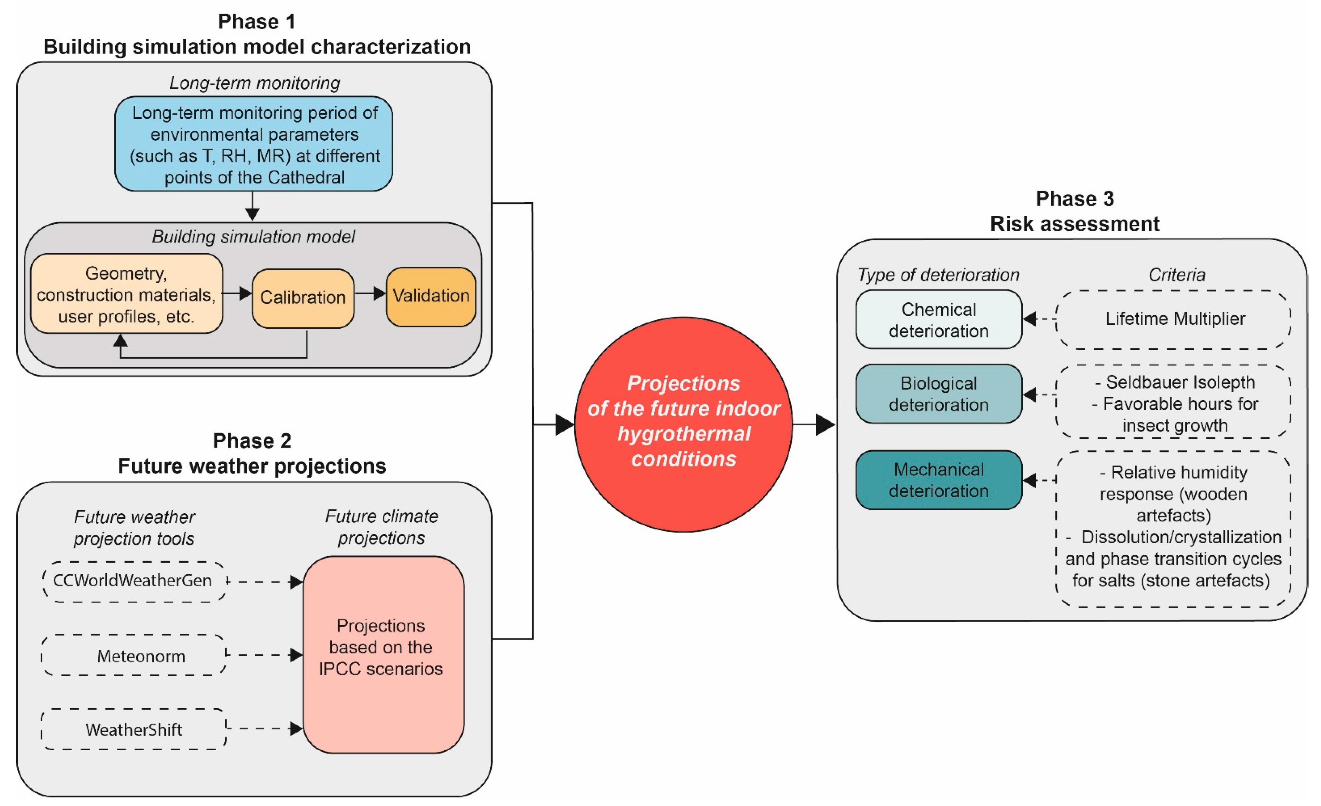
2. Method, Tools and Risk Assessment Criteria

The method developed and applied in the research work is divided into three main phases. In the first one, the monitoring of the building indoor climate must be performed. It allows us to characterize the current indoor climate condition and, subsequently, to validate the simulation model necessary to carry out future projections. In the second phase, to assess the impact of climate change on the built environment, it is necessary to define some possible future scenarios. In that respect, the projections made by the Intergovernmental Panel on Climate Change (IPCC) [27] have been adopted in the building simulation, through the creation of future climatic files with a weather generator tool. Finally, in the third phase, through the validated model and the abovementioned climatic data, the future indoor conditions can be forecasted to evaluate the impact of climate change on the conservation of artworks contained in a certain building. Within such a phase, three main categories of deterioration risk have been evaluated: chemical, biological, and mechanical. The method adopted in this research work is outlined in Figure 1, while the detailed description of each phase is described in the next sections.

2.1. Building Simulation Model Characterization (Phase 1)

In this section, the two steps necessary to characterize and validate the simulation model are described.

2.1.1. Long-Term Monitoring

In heritage buildings, particularly those not equipped with a heating, ventilation, and air conditioning (HVAC) system, the monitoring of indoor climate parameters, such as the air temperature, relative humidity, etc., is an important step that allows us to characterize their hygrothermal behaviour and carry out different evaluations [28]. In the proposed method, on-site microclimate monitoring represents a pivotal step for the model calibration and validation to carry out reliable projections [29]. In such a respect, the main climatic parameters, such as the air temperature and relative humidity, should be monitored for a period sufficiently long (at least one year) with an hourly interval, to properly compare the simulation output with the real data for different seasons and conditions [28].

Moreover, in heritage buildings characterised by particularly huge volumes [30], multiple significant points inside the space should be identified and monitored; this allows us to detect possible hygrothermal stratifications and to determine the average behaviour of the environment, useful for comparison with the simulation results.

2.1.2. Building Simulation Model

The indoor climate of new and existing buildings can be predicted through building simulation models, which can forecast their energy and environmental performance according to different boundary conditions [2]. In literature, several tools are adopted, among them the most used are EnergyPlus, DesignBuilder, Trnsys, Wufi Plus, etc. [31].

When dealing with heritage building simulation, some limitations that increase the output uncertainty can be highlighted according to some recent publications [31] (e.g., the lack of information regarding input parameters, the limitations of the tools to describe the geometric features, etc.). Despite these limitations, building simulation models represent one of the most powerful methods to forecast building behaviour. However, it is pivotal that such models are calibrated and validated against real measurements in order to obtain reliable predictions [2,32].

The calibration includes the process of adjusting physical modelling parameters in the simulation model to improve the agreement with experimental data. In such a respect, in Section 3.3, the most influencing input parameters are described.

Regarding the model validation, to assess the level of accuracy some statistical indices must be calculated. Such indices are the Root Mean Squared Error (RMSE) and the Pearson correlation coefficient (r), calculated through the following equations:

$$RMSE=\sqrt{\frac{{\sum }_{i=1}^n{(m_i-s_i)}^2}{n}}$$

(1)

$$r=\frac{{\sum }_{i=1}^n(m_i-\overline{m})(s_i-\overline{s})}{\sqrt{{\sum }_{i=1}^n{(m_i-\overline{m})}^2}\sqrt{{\sum }_{i=1}^n{(s_i-\overline{s})}^2}}$$

(2)

where,

• m_i and s_i are the measured and simulated values, respectively;
• $\overline{m}$ and $\overline{s}$ represent the average of the measured and simulated data, respectively;
• n is the number of total data.

Both statistical indices must be calculated for three main climatic parameters: temperature (T), relative humidity (RH), and mixing ratio (MR). The result of these indices have to be compared against validation thresholds defined by some protocols/standards [33,34,35] and by technical literature [32]:

• RMSE ≤ 1 °C for temperature, ≤5% for relative humidity, and ≤1 g/kg for mixing ratio referred to accurate simulation models (LIV 1), according to [32];
• r² > 0.75, as suggested in [29,33,35].

A further verification is related to the frequency of residuals (differences between measured and simulated data for each time step), verifying that a sufficiently high amount of them are below a suitable threshold. In detail, the thresholds proposed by [29] for each of the three parameters analysed are ±1 °C, ±5% and ±1 g/kg (LIV 1) and ±2 °C, ±10% and ±2 g/kg (LIV 2), respectively, for T, RH, and MR for at least the 95% of the residuals inside one of these two accuracy levels. A detailed description of the model validation is shown in Section 3.3.2.

2.2. Future Weather Projections (Phase 2)

As already introduced, to carry out risk projections, the reference climatic scenarios must first be defined. In such regards, the Fifth Assessment Report (AR5) of the IPCC, which provides different scenarios called Representative Concentration Pathways (RCPs), can be used as a reference. Such scenarios are described as follows:

• RCP 8.5 scenario is the one with the highest emissions and represents the situation we are in today. In this scenario, emissions are projected to increase continuously throughout the XXI century;
• RCP 6.0 and RCP 4.5 are two intermediate scenarios, where the emissions will be reduced through the implementation of strategies and technologies. For scenario RCP 6.0, the peak of the emissions is reached in 2080, while for RCP 4.5 in 2040;
• RCP 2.6 represents a situation where the emissions peak starts in 2020. The concentration of GHGs gradually decreases, such as the amount of heat retained by the atmosphere.

Each of these scenarios corresponds to projections of how much greenhouse gases will be emitted to the atmosphere and, therefore, how much the temperature and sea levels will rise. To implement such scenarios in building simulation and carry out future projections, tools or models able to generate future climate weather files are necessary. These tools are called future weather generators and are based on different downscaling procedures of climate models [36]. The downscaling process of Global Climate Models (GCMs) provides climate data with higher spatial and temporal resolution. This procedure needs further information and assumptions, which generally cause propagation of uncertainties, e.g., uncertainties in the historical relationship between temperature variability and economic growth, the spatial pattern temperature change associated with the level of aggregate emissions and the future rate and pattern of economic development. However, there is significant confidence that climate models provide reliable quantitative estimates of future climate change [36].

Some of the most widely used tools are Climate Change World Weather Generator (CCWorldWeatherGen) [26], Meteonorm [37], and WeatherShift [38]. They are based on different IPCC reports and allow generating various scenarios for different periods of the XXI century; furthermore, some of them allow creating the future climatic file starting from one chosen by the user. According to Moazami et al. [36], the results provided by weather files generated by statistical methods can be sufficient to provide enough information to study the long-term shift in energy use of buildings.

Climate Change World Weather Generator is a tool developed on Microsoft Excel by Jentsch et al. [26] based on IPCC Third Assessment Report. This tool allows the transformation of “current” climate files into the future ones, based on the IPCC’s most unfavourable scenario.

Meteonorm software provides a database of weather files of any location in the world. This tool can create future climate files for IPCC scenarios RCP 2.6, 4.5, and 8.5 for a period that ranges from 2020 to 2100 with ten-year intervals [37].

WeatherShift is a web platform developed by Arup and Argos Analytics for the visualization and generation of future meteorological files, based on the emission scenarios RCP 4.5 and RCP 8.5 [38], and this tool provides the climate file for three periods (2035, 2065, and 2090).

In this study, the WeatherShift tool is adopted for future weather file generation, since it is based on the latest release of IPCC projections for the most unfavourable emission scenario (RCP 8.5) and an intermediate one (RCP 4.5). WeatherShift applies the morphing downscaling method to the outcomes of 14 GCMs available with the AR5 [36]. The morphing is a statistical method that applies three transformation algorithms to the weather variables (shift, stretch, and a combination of both) to adjust them and create future climate weather files. The algorithms apply changes based on monthly trends and variations of GCM or Regional Climate Model (RCM) outputs for a given location [36].

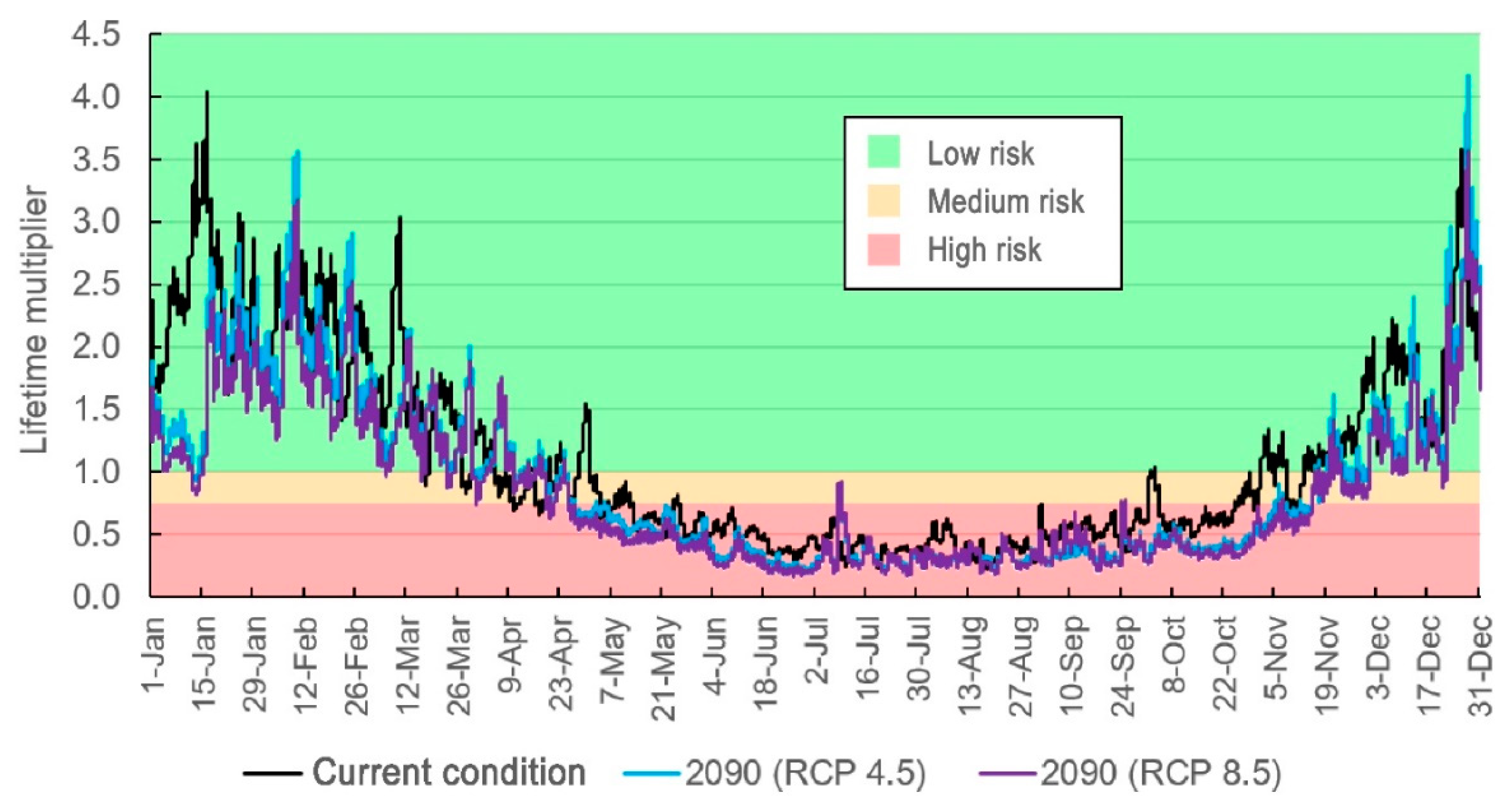
2.3. Risk Assessment (Phase 3)

Criteria widely used in the literature have been adopted in the proposed methodology, to evaluate the risks of deterioration for building materials and artworks [39,40,41]. These criteria are based on different causes of the deterioration: chemical, biological, and mechanical. Furthermore, in the literature exist other methods that use risk indexes to assess the threat level for the deterioration of the artworks [42,43], which are based on suitable T-RH intervals for artwork preservation according to standards and protocols [44,45,46,47].

In the next subsections, a description of criteria that will be applied to measure the risk level of the case study in Section 4.2, has been provided.

2.3.1. Chemical Deterioration

The chemical degradation is generally related to the deterioration of the cellulose of paper and the yellowing of protective varnish on paintings.

The criteria adopted allows us to define the rate of chemical deterioration based on temperature and relative humidity to calculate the so called Lifetime Multiplier (LM) [48]. Such a parameter estimates the life expectancy of the material, compared to the case of maintaining the object in an environment with temperature and relative humidity fixed at 20 °C and 50%, respectively. The LM is calculated according to the equation hereafter reported:

$$L{M}_i={\left(\frac{50\%}{R{H}_i}\right)}^{1.3}\times e^{\frac{E_a}{R}\times \left(\frac{1}{(T_i+273.15)}-\frac{1}{293.15}\right)}$$

(3)

where,

• LM_i is the Lifetime Multiplier at instant i [-];
• E_a is the activation energy [J/mol];
• R is the universal gas constant [8.314 J/molK];
• T_i is the air temperature at instant i [°C];
• RH_i is the relative humidity at the instant i [%].

The activation energy varies according to the material and consists of the energy required for a chemical reaction to take place. This energy ranges from 70 to 100 kJ/mol for most materials; specifically, it is 70 kJ/mol for the yellowing of varnishes and 100 kJ/mol for the degradation of cellulose [48].

To obtain a global value of LM, representative of the risk condition for the entire year analysed, the equivalent Lifetime Multiplier (eLM) can be calculated, according to the equation provided by H.E. Silva et al. [49], shown below.

This indicator represents an average of the reciprocal values of the individual LM calculated for each interval.

$$eLM=\frac{1}{\frac{1}{n}\times {\sum }_{i=1}^n\frac{1}{L{M}_i}}$$

(4)

where,

• eLM indicates the equivalent Lifetime Multiplier [-];
• n is the number of total data [-].

Finally, three main classes of risk associated with eLM values can be identified [40,50], as shown in

Table 1. Risk levels associated with eLM values.

Risk Level	Range
Low risk	eLM > 1
Medium risk	0.75 < eLM ≤ 1
High risk	eLM ≤ 0.75

.

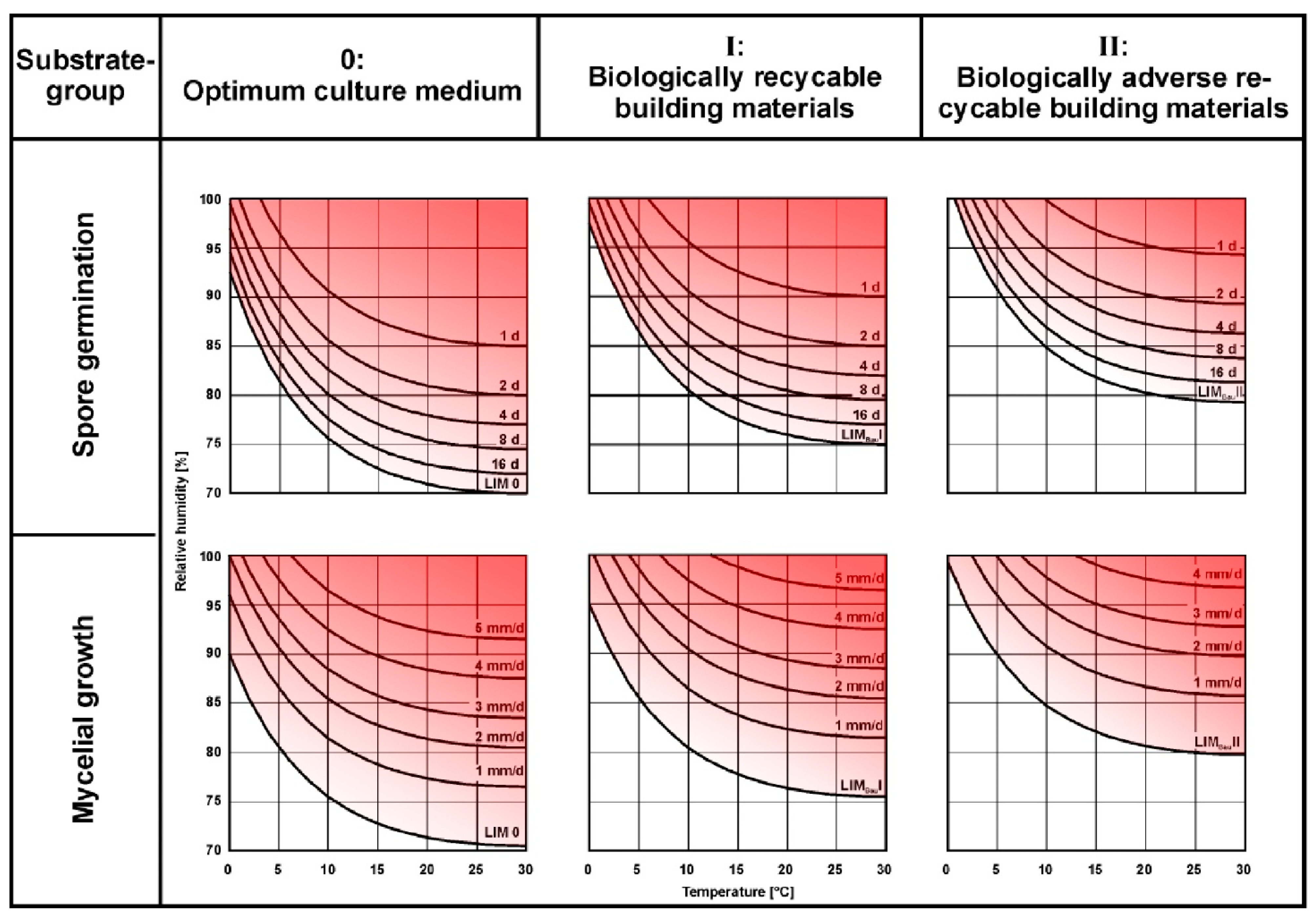
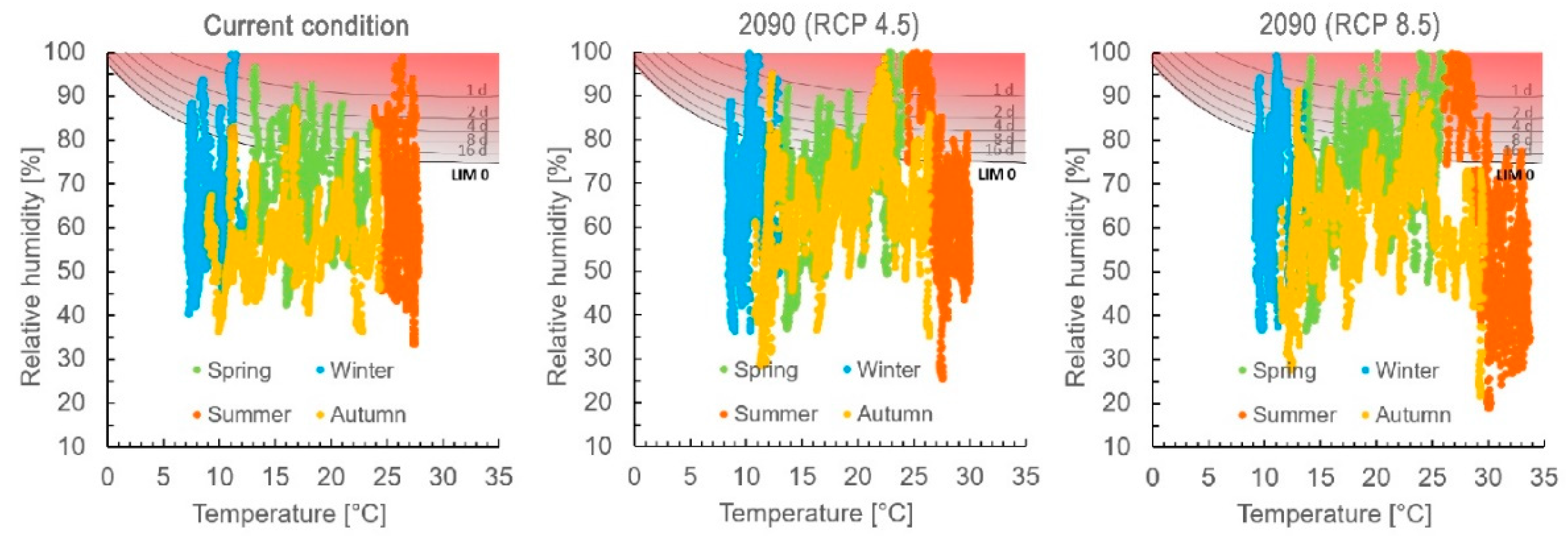
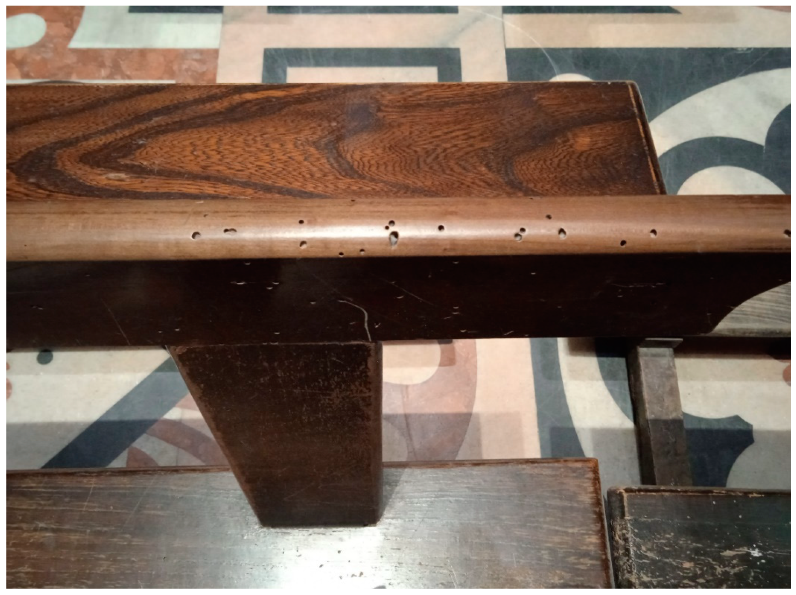
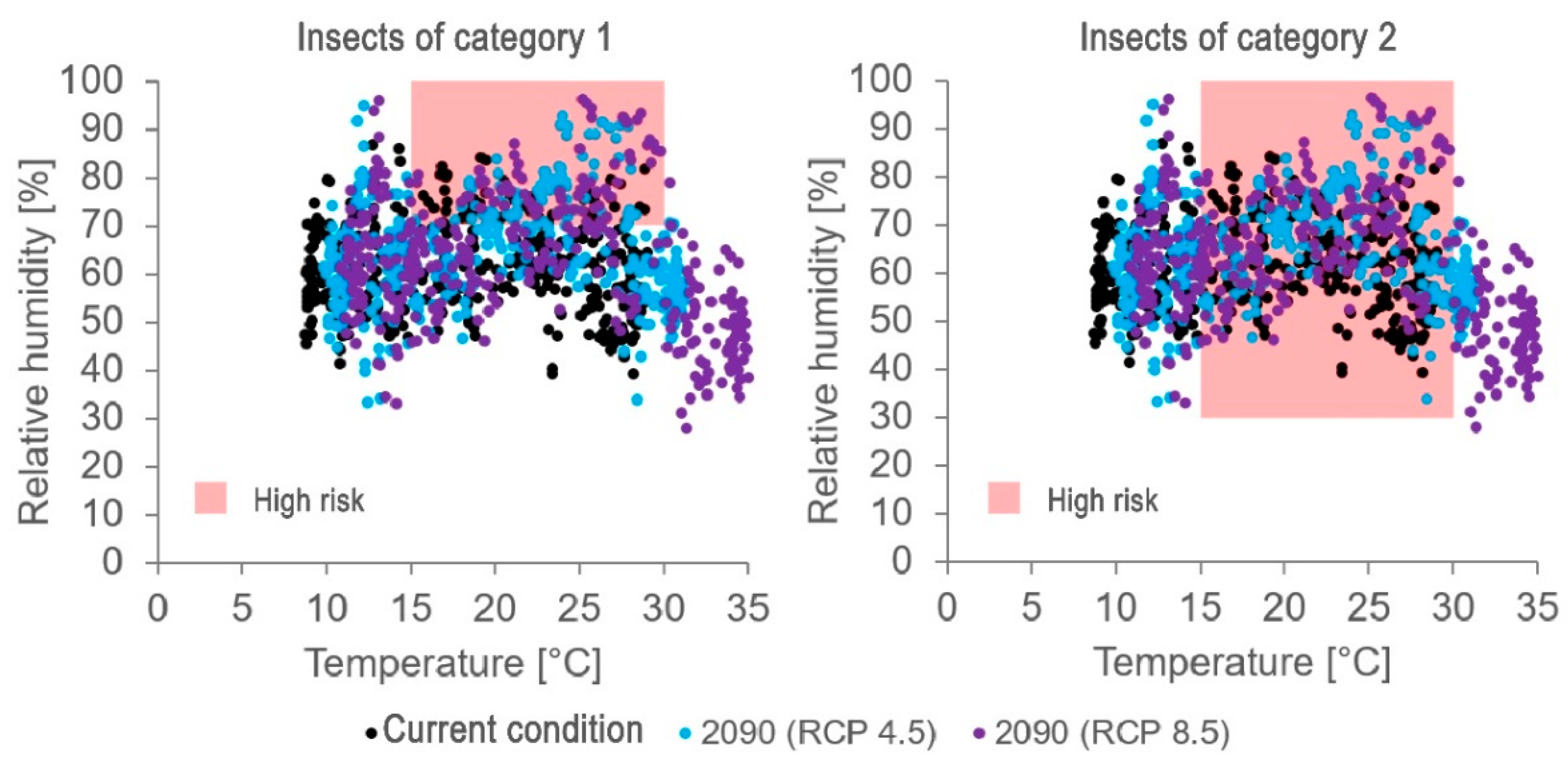
2.3.2. Biological Deterioration

In the building sector, biological deterioration (caused by mould growth, pest proliferation, etc.) represents a risk to both the preservation of the building and the health of the occupants. The Seldbauer’s Isopleth system [51] is one of the most widely used methods in the literature to evaluate mould risks [52]. This method is based on the relationship between surface temperature, relative humidity, and exposure time, which are considered the main factors inducing the mould growth process. This relationship is expressed through isolines that represent the number of days required for mould germination and quantify mycelium growth based on microclimatic conditions.

The rate of growth of a mould spot (diameter), is measured in mm/day or mm/year [51]. Seldbauer distinguishes four categories of the substrate (

Table 2. Assignment of different materials to substrate categories.

Substrate Category	Representative Materials
0	Biological complete media
I	Wallpapers, plasterboard, building products of easily degradable raw materials, material for permanently elastic joints
II	Plasters, mineral building materials, some woods, insulants not belonging to group I
III	Metals, foils, glass, tiles

) where mould can grow at different rates under the same temperature and relative humidity conditions [51].

It should be noted that, in cases where there is considerable dirt and dust on surfaces, substrate category I should be assumed instead of classes II and III [53]. The lowest isoline, where no germination or spore growth is expected, is called LIM (Lowest Isopleth for Mould), as shown in Figure 2.

In order to assess the risk of mould germination, the germination factor (GF) can be calculated as the ratio between the total continuous period of exceedance of an isoline and the time for spore germination specified for a specific curve [39]. To have a more accurate prediction, the isolines can be interpolated. When the GF exceeds the value of 1, spore germination occurs and from that instant, the mould will continue to grow at a speed that depends on climatic conditions.

Finally, three main levels of risk associated with mould growth, evaluated over the whole year, are shown in

Table 3. Risk levels associated with mould growth in a year.

Risk Level	Range
0	Mould growth ≤ 50 mm/year
I	50 mm/year < Mould growth ≤ 200 mm/year
II	Mould growth > 200 mm/year

[54]. However, if the GF never reaches the value of 1 during the analysed period, no risk of mould growth is expected.

Insects can be another cause of damage to materials. Such damage can be caused in organic materials (such as paper and wood) and on some fabrics, by particular types of insects [13]. The main factors considered to assess the risk of insect damage are the climate conditions (air temperature and relative humidity).

In this study, to assess the impact of deterioration risks caused by insects, the percentage hours in a year favourable to their growth are calculated. It should be noted that insect growth increases when the temperature conditions remain in the favourable ranges for a continuous period and with the increasing of temperature [55]. In detail, two particular categories of insects have been analysed, which correspond to two different environmental conditions suitable for their growth [18]:

• Category 1: RH > 70% and T between 15 and 30 °C for insects such as silverfish, psocoptera, and woodworms;
• Category 2: RH > 30% and T between 15 and 30 °C for insects such as the drugstore beetle and the clothes moth.

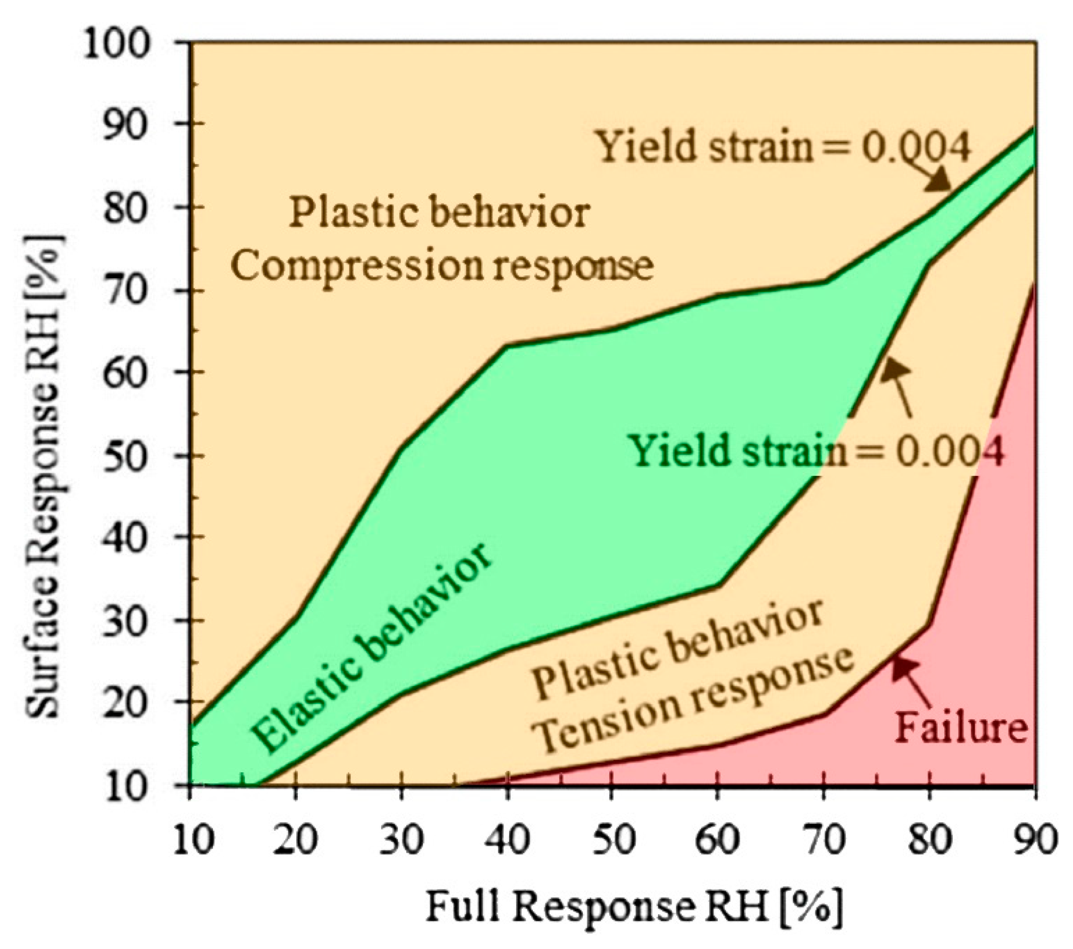
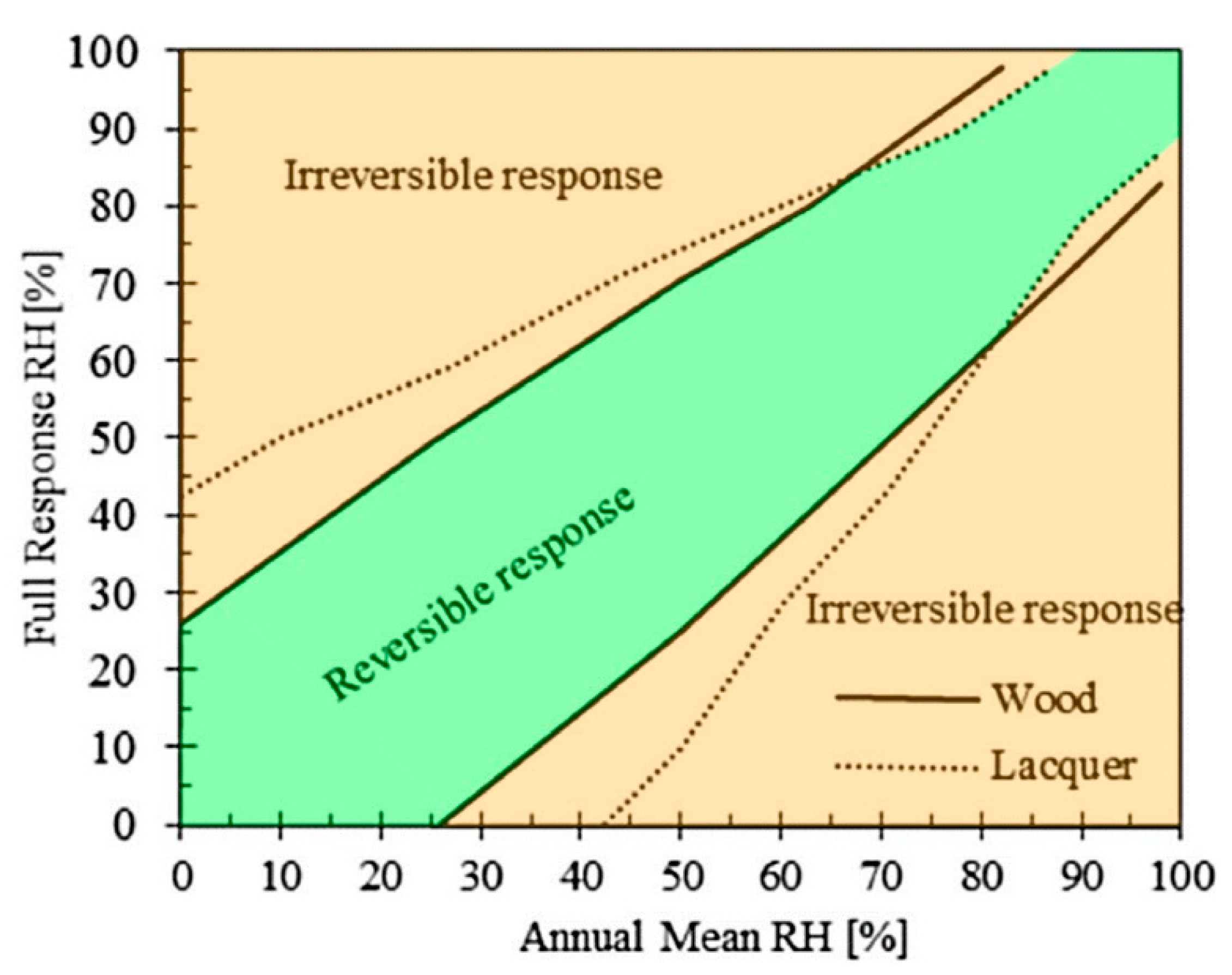
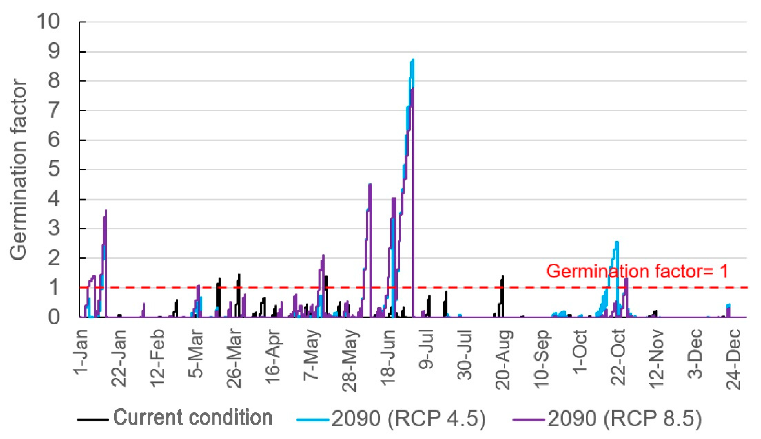
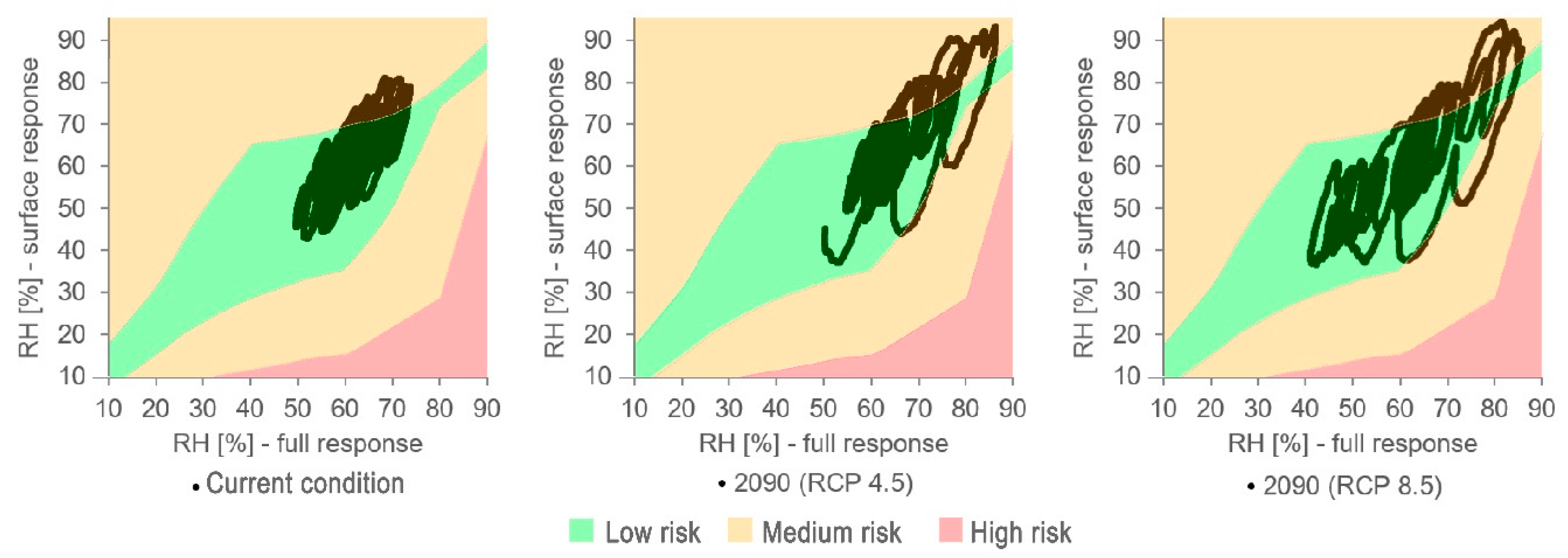
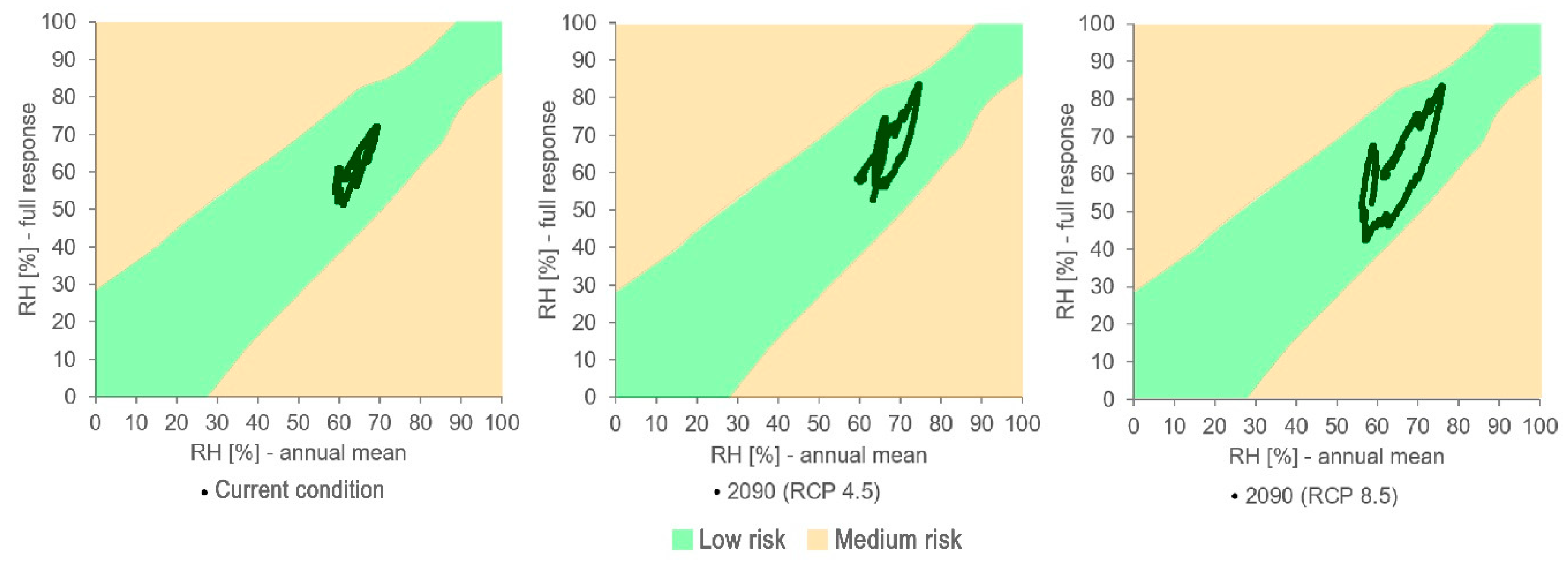
2.3.3. Mechanical Deterioration for Wooden Objects

Mechanical degradation in hygroscopic organic materials (such as paper, wood, etc.) depends primarily on fluctuations in relative humidity that changes the moisture content causing dimensional variations, which can lead to internal stresses (cracks, detachment of surface material, etc.) [39]. Generally, RH fluctuations do not have an immediate effect on the materials, taking some time (hours, days or even weeks) to reach an equilibrium with the surrounding environment, depending on their water vapour adsorption/desorption characteristics [49]. Moreover, it should be noted that the material interior and surface layer need a different time to adapt to RH fluctuations and for already damaged objects that time can decrease [40].

In such a respect, in

Table 4. Relevant responses and corresponding response times for different objects, according to [39].

Object	Relevant Responses	Response Time
Panel painting	Surface response just under oil paint	4.3 days
	The full response of the entire panel	26 days
Lacquer wooden box	The full response of the entire lacquer box	40 days

, the time necessary for different objects to adapt themselves to changes in RH are provided [39]. Such response times have been evaluated experimentally for some specific objects [39,56,57]. The following reference values have been adopted to carry out a general assessment.

The criteria to assess the risk of mechanical degradation for some wooden objects is based on the relative humidity response (RH_response), which is defined as the RH of the object assuming that at the end of the response time, the object reaches an equilibrium with the environment. The RH_response of objects at a generic instant i can be calculated through the following equation [39]:

$$R{H}_{response,i}=\frac{a\times R{H}_i+a^2\times R{H}_{i-1}+a^3\times R{H}_{i-2}+a^4\times R{H}_{i-3}+\dots }{\frac{a}{\left(1-a\right)}}$$

(5)

where,

• RH_response,_i is the relative humidity response at time i [%];
• RH is the relative humidity of the environment [%];
• i is the current time within the data set [-];
• a is the response factor [-].

In order to take into consideration the response time of materials, the response factor (a) is calculated through the following formula:

$$a=e^{\frac{-3\times \Delta t}{t_{response}}}$$

(6)

where,

• Δt indicates the time-step interval in seconds [s];
• t_response is the response time, after the conversion in seconds of the days indicated in Table 4 [s].

Through the calculation of the RH_response, the risk of mechanical damage on painted wooden panels and furniture can be assessed. In detail, for painted wooden panels, the diagram proposed by Mecklenburg et al. [58] based on the yield deformation criteria, which combines the surface and full material response to RH variation in the environment, is adopted (Figure 3). In this method, the differential deformations between the surface and the whole object, based on fluctuations in relative humidity, are analysed.

In detail, Figure 3 shows areas where the response of the surface and the whole wood panel causes elastic and reversible dimensional deformations (area indicated as “elastic behaviour” in Figure 3). When fluctuations exceed from the “elastic behaviour” area, deformations become irreversible, increasing in magnitude as the RH fluctuations distribute deeper in the area indicated as “plastic behaviour compression response” or “tension response”. Finally, when the environment becomes too dry, the RH_response can reach the “failure” area in Figure 3, causing visible cracks in the material [59].

Regarding furniture, the diagram proposed by Bratasz et al. [57] in a study on the dimensional response to changes in relative humidity of a lacquered wood box has been adopted. Similarly to wood panels, the admissible response of the wooden box is based on the yield deformation criteria, which allow us to define the “reversible response area” for both materials (wood and lacquer). In Figure 4, the x-axis indicates the mean annual response [39], while the y-axis indicates the whole response of the object [57].

2.3.4. Mechanical Deterioration in Masonry

The study of the effects of salts in masonry is a complex problem that depends not only on climate conditions but also on the characteristics of the material itself, sources of salts, etc. [15]. However, in this study the objective is to obtain a general trend using a method to assess the risk of damage caused by salts in masonry mainly based on climate variations [21,60,61].

In detail, the cycles of crystallization and phase change of some diffused salts in masonry should be analysed. The first salt that deserves to be analysed is sodium chloride (NaCl), found in the mineral form of Halite; for this salt, the number of times when the daily average relative humidity exceeds and returns below the critical RH value of 75.3% is counted, since it activates the process of deliquescence and following recrystallization [60].

The second salt is sodium sulphate, found in the form of Thénardite and Mirabilite. The transition phase from Thénardite to Mirabilite (Na₂SO₄→Na₂SO₄⋅10H₂O) occurs due to the inclusion of 10 water molecules in the hydrated crystal. The RH_critical value for the phase transition is obtained by the following equation [59]:

$${\mathrm{RH}}_{critical}=0.8485\times {\mathrm{T}}_s+60$$

(7)

where T_s is the surface temperature, between 0 and 30 °C [59].

When the RH exceeds the critical RH threshold, the transition from Thénardite to Mirabilite occurs, causing high pressure within the pores of the material, resulting in deterioration. Repeated cycles cause an accumulation of stresses that can cause severe material decay.

Within the European project Climate for Culture [13,18], certain risk levels are defined based on the number of transition cycles that occur in a year, as shown in

Table 5. Risk levels associated with the number of transition cycles per year for the Halite, and the Thénardite and Mirabilite.

Risk Level	Range
Low risk	Cycle/year ≤ 60
Medium risk	60 < Cycle/year ≤ 120
High risk	Cycle/year > 120

. Such thresholds have been adopted even for Halite deliquescence and recrystallization cycles.

3. Case Study and Simulation Model

The described methodology has been applied to the Duomo di Milano, one of the largest historic buildings in Italy. This section reports a brief description of the main building characteristics, the on-site monitoring campaign of the climatic parameters, and the calibration and validation process of the simulation model.

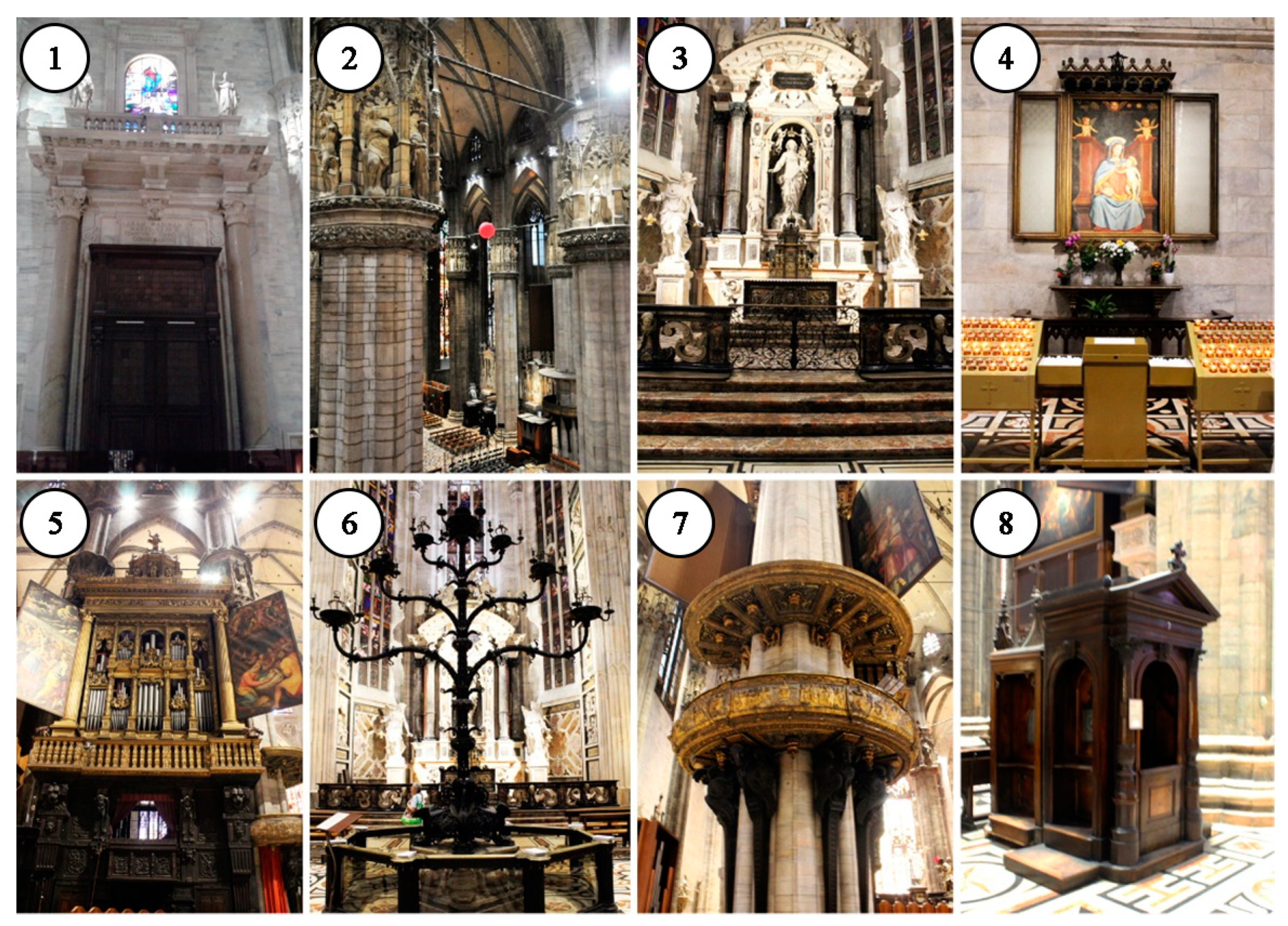
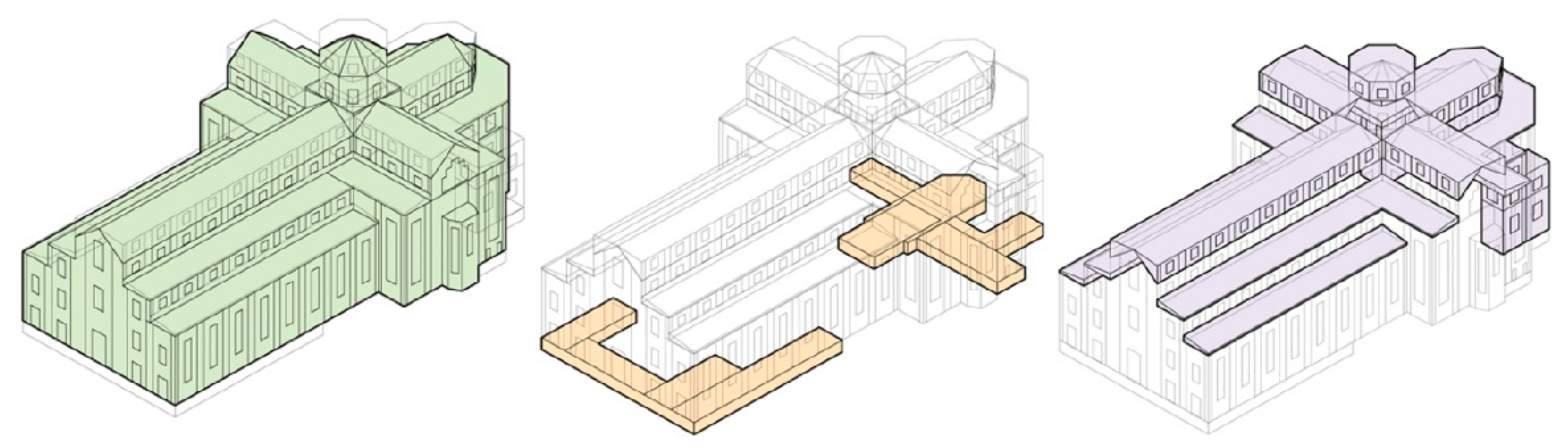
3.1. Brief Description of the Building

The indoor space of the Duomo di Milano occupies an area of 8500 m² and a volume of approximately 300,000 m³, with internal heights that vary from 20 to 45 m, respectively, for the lateral and central naves, up to 65 m at the cupola. The building envelope is made with masonry walls having a variable thickness between 1 and 5 m, approximately.

There are over 50 stained glass windows, decorated with the grisaille painting technique. The roof construction system has a double system of overlapping brick vaults that form accessible attic spaces called “sordine”. These areas are directly connected with the interior of the cathedral, thanks to numerous ventilation holes.

The openings (doors and some portions of the windows) are managed in two different ways depending on the period of the year, to increase or decrease the air exchanges with the outdoor. In the first operating condition (adopted for most of the year), all the openings, except for visitors access, are kept close. In the second, adopted exclusively in the summer months (about from June to September), to increase natural ventilation, some windows in the ambulatory and the transept are kept open, as well as the doors on the main front with their respective fanlight.

Furthermore, inside the Cathedral there are also numerous artefacts of various types, ages, and materials; some of them are shown in Figure 5. The marble is the finishing layer of the envelope and it is one of the main materials for numerous sculptures and decorations (n° 1, 2 e 3 in Figure 5). Another common material is the wood, used for example for the benches, confessionals (n° 8 in Figure 5), the choir seats, and the organ cases, one of which has large wooden panels painted (n° 5 in Figure 5). Under the tiburium, suspended on the two terminal pillars of the nave, there are the pulpits, formed by bronze caryatids supporting a balcony with gilded copper balusters (n° 7 in Figure 5).

In the numerous altars of the aisles, there are also various artefacts of different origins and materials (n° 3 e 4 in Figure 5).

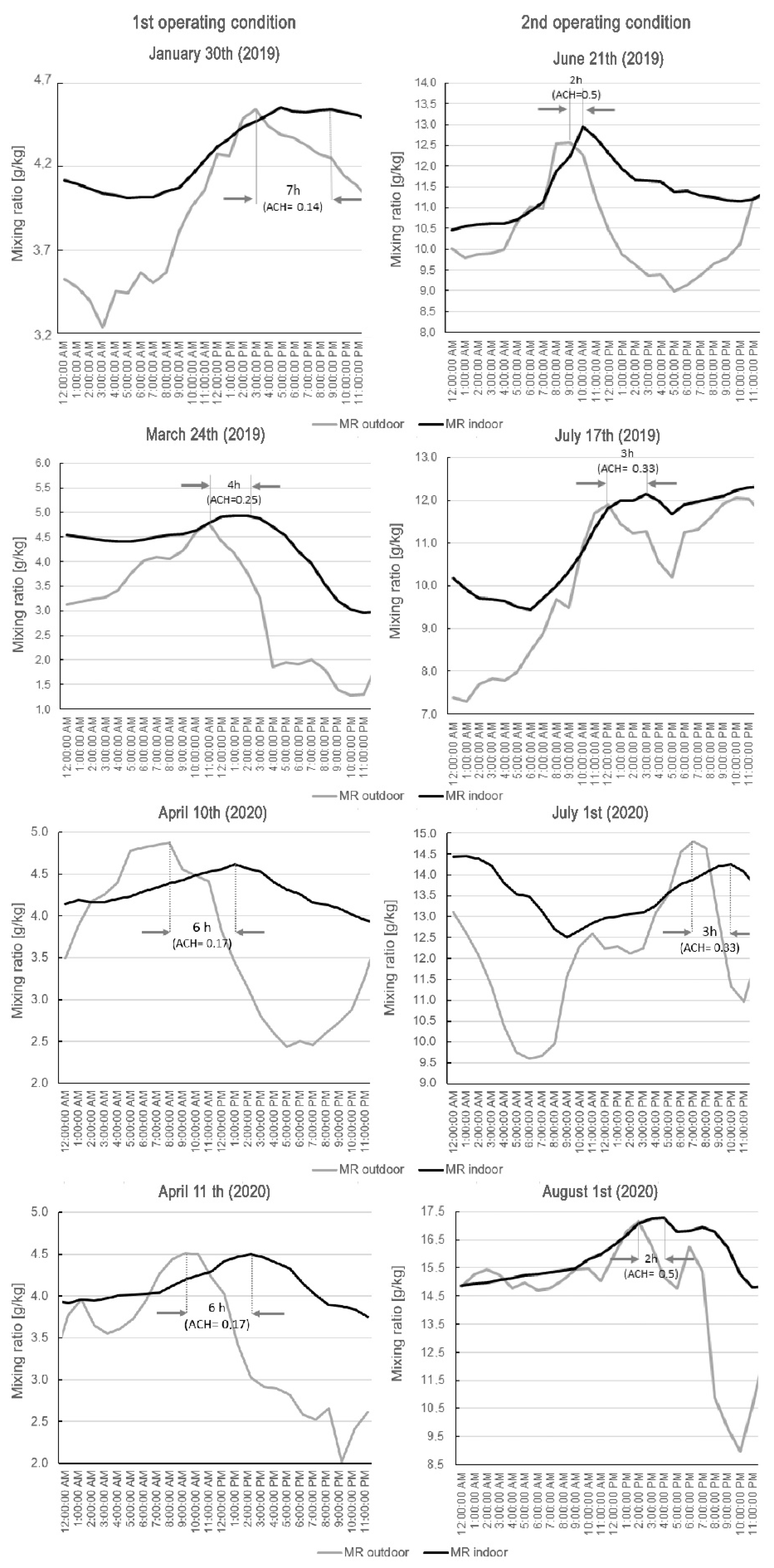
3.2. On-Site Indoor Climate Monitoring

As already said, the monitoring campaign should be considered the starting point to obtain reliable data from the simulations. In the literature, several methods and tools have been used for the monitoring of historic buildings [62,63,64,65,66,67,68,69]. In that respect, the collection of the indoor climatic data started in February 2016 and was divided into two phases. In the first, a series of punctual measurements were carried out through the use of a probe balloon equipped with wireless sensors, which allowed the mapping of the main microclimatic parameters, in order to identify possible stratifications of temperature and humidity. In the second, a long-term measurement plan was defined, which included the installation of several datalogger sensors (Hobo MX T/RH data logger), in the most relevant points previously identified. The detailed monitoring campaign as well as the main results are described in a previous publication [67].

3.3. Duomo di Milano Simulation Model

As already introduced, the impact of climate change on the indoor environment of buildings can be assessed through simulation models properly validated against real data. In this study, the software EnergyPlus v8.9 [70] was adopted to carry out the microclimate simulations.

3.3.1. Characterization and Calibration

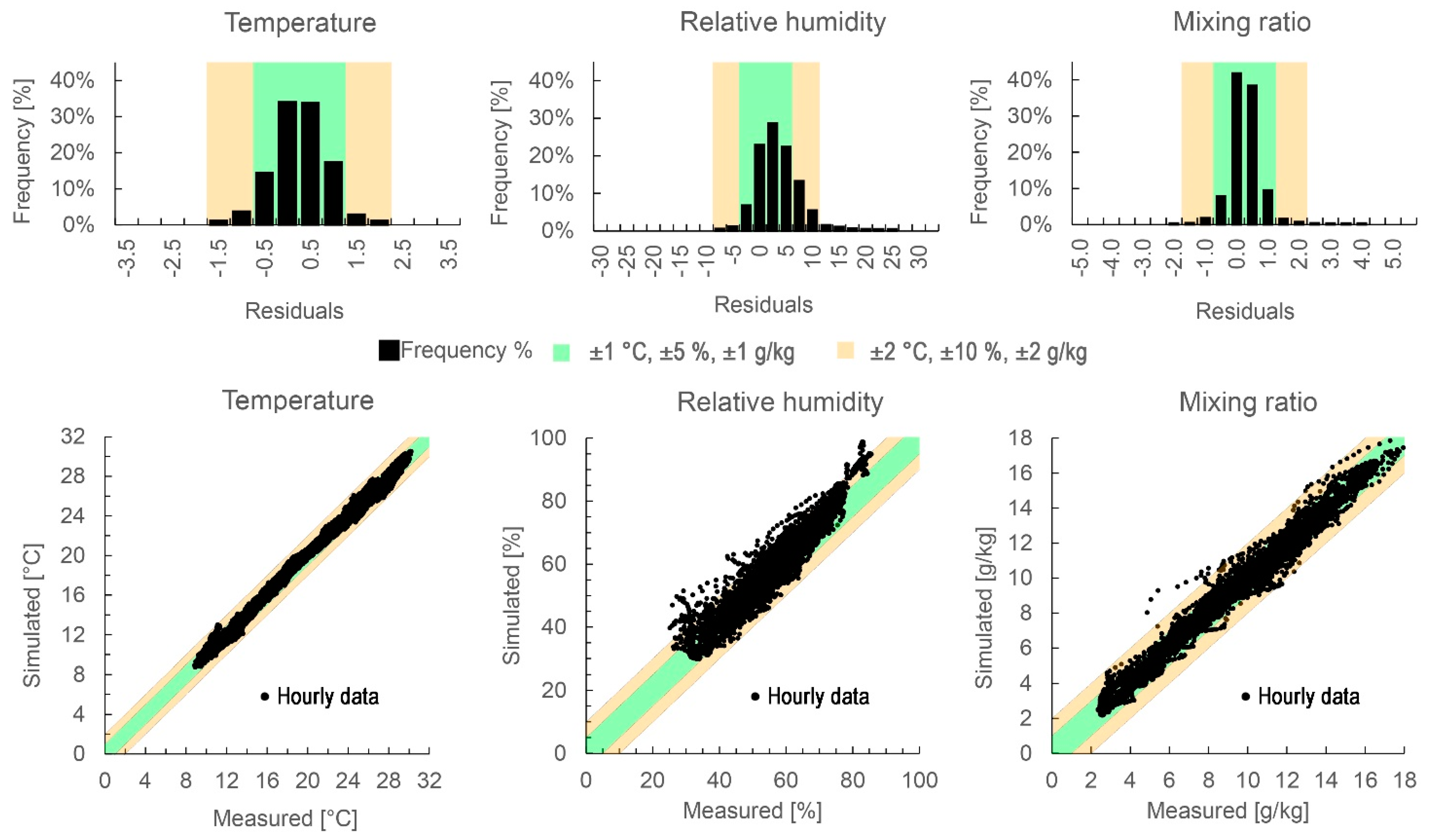
Given the great complexity that characterises the Cathedral of Milan, the modelling required a process of simplification of the spaces and the geometries. A total of 20 thermal zones were created, divided between the main environment of the cathedral, the basement spaces, the areas in the roof called “sordine,” and the sacristies (Figure 6).

The building is not equipped with an HVAC system, thus, the simulations were performed in free-floating conditions. The operation of the cathedral during the year were implemented in the model through some schedules with the occupation profile, internal loads for artificial lighting, and natural ventilation conditions.

The Duomo di Milano is made of dry masonry walls, with U-values estimated to range from 0.29 to 0.92 W/m²K depending on the thickness. The particular high wall thicknesses cannot be successfully simulated with the standard algorithm implemented in EnergyPlus for heat transfer calculation called Conduction Transfer Function [71]. However, adopting the Conduction Finite Difference algorithm [71,72], it is possible to perform the simulations, but at the expense of calculation time. Both algorithms were used progressively in this study. In detail, with the standard algorithm, the masonries having a maximum thickness allowed by the software have been processed, applying an equivalent transmittance of the real wall (the remaining mass has been inserted as internal mass). The simulations performed through this procedure allowed us to calibrate the simulation model faster. The second algorithm was used to carry out the final fine-tuning of the model and to fully take into account the thermal inertia of the building.

The roof system is characterised by a double system of vaults made of solid bricks with a U-value estimated to be 1.17 W/m²K.

Regarding the transparent envelope, these are characterised by a complex geometry that was simplified and modelled considering only the glass surface, adopting a U-value of 5.8 W/m²K [31]. The solar heat gain coefficient (SHGC) and the visible transmittance (τ_v) were adopted from a study carried out on some ancient stained glass decorated with different surface techniques [73]. These values are equal to 0.15 and 0.1, respectively, for SHGC and τ_v.

The method adopted to estimate the air change per hour (ACH) is based on the analysis of indoor climatic data. The ACH from natural ventilation and infiltration in historic buildings is one of the most important parameters that affect the simulation results [31,74]; however, it is difficult to assess due to the huge volume that generally characterizes such structures.

In that respect, the indoor climatic data of the Duomo di Milano has been adopted to estimate air changes through a graphical comparison of the indoor and outdoor mixing ratio (MR), as suggested by the ASHRAE Guideline 34-2019 [47].

In detail, in the method proposed by the ASHRAE regulation, parameters such as absolute humidity, mixing ratio, vapour pressure, etc., can be considered as “tracer gases” that are absorbed or desorbed from the surrounding environment. Hence, through the comparison of internal and external MR values, the air change rate with outdoor can be estimated by counting the hours (time step of the measurements) between the external and internal MR peaks.

However, it should be noted that using such a method it is difficult to isolate the effect due to indoor sources of moisture (e.g., people, etc.) [47].

In that regard, two years have been analysed, one before and one during the Covid-19 pandemic, respectively, 2019 and 2020. In 2020, the particular conditions caused by Covid-19 reduced the presence of visitors inside the Cathedral [75], allowing the recording of the indoor climatic data over a long period, with a negligible or null human effect. Conversely, 2019 represents a pre-pandemic year, characterised by a high number of visitors. The analysis of 2019 is, thus, pivotal to evaluate the impact of people’s presence on indoor environmental conditions.

As discussed in Section 3.1, two different operating conditions of the openings (the first adopted for almost all the year while the second adopted just during the summer months) are implemented in the Duomo, thus, the ACH has been estimated for both cases.

In Figure 7, the trends of the estimated ACH for some sample days of 2019 and 2020, according to the different conditions, are shown.

According to the data acquired along the monitored period, it can be noticed that, for the first operating condition, adopted for the main part of the year, the estimated average ACH are equal to 0.26 and 0.22 for 2019 and 2020, respectively. While for the second operating condition, adopted during the summer months, the average ACH are equal to 0.37 and 0.33 for 2019 and 2020, respectively. The higher ACH of the second operating condition mainly depends on the larger openings surface available in the summer months, as described in Section 3.1.

From the comparison of the data related to the two years analysed, it can be stated that the yearly average ACH is about 11% higher in the year before the Covid-19 pandemic. Such difference is partially related to the impact of people in terms of moisture production, but also to the additional air exchange from the continuous opening of the entrance/exit doors, which influences the indoor mixing ratio.

However, it should be noted that such a small difference indicates that the number of people, although high, has a limited impact on the indoor climate, mainly related to the huge volume of the Duomo. Thus, due to the similarity between the two years, the ACH values related to 2019, which are representative of the standard occupancy of the building, are adopted.

The outdoor MR was obtained from the Brera meteorological station of ARPA [76], placed a few hundred meters from the Duomo di Milano, while for the indoor MR the data logger located in a central point of the cathedral was considered.

Regarding internal heat loads due to people, an occupancy density of 0.11 people/m² was defined (corresponding to an average value of 9000 visitors per day distributed in 10 h of operation, as recorded in the cathedral during the weekdays), while for the internal loads due to artificial lighting, 2 W/m² have been assumed for the current LED lighting system of the Cathedral [77]. Finally, the internal mass of the 52 columns was also implemented.

Once the main characteristics of the model were defined, simulations were performed and their results were compared with the data collected during the monitoring campaign for 2019. As introduced, this year was selected because it is representative of the normal operation of the Cathedral and the indoor climatic data were collected without interruption. Moreover, it should be noted that for the model calibration and validation, the hourly average value of all the probes installed was used. Such data were preferred instead of using just one probe, since it better represents the general behaviour of the indoor environment and not only a localised area.

3.3.2. Validation

In the simulation of existing buildings, the accuracy of the model plays a crucial role to obtain reliable evaluations [32] and it can be measured with the statistical index [78]. In detail, the calculated values of RMSE and r² of the simulation model are within the thresholds described in Section 2.1.2, as reported in

Table 6. Indexes RMSE and r² for T, RH, and MR of the validated model.

	T	RH	MR
RMSE [°C, %, g/kg]	0.52	4.21	0.45
r2 [-]	0.993	0.904	0.984

.

Moreover, in Figure 8, a graphical comparison of the simulated and measured temperature, relative humidity, and mixing ratio is reported. Such charts show the frequency of residuals and the scatter plot comparison between hourly measured and simulated data. For each of the three parameters analysed, two accuracy levels are reported: ±1 °C, ±5% and ±1 g/kg (LIV 1) and ±2 °C, ±10% and ±2 g/kg (LIV 2), respectively, for T, RH, and MR, according to [29].

In detail, about 95% of the residuals are within LIV 1 for temperature, while the remaining 5% is within the range of LIV 2. The mixing ratio has a similar distribution, with 96% of residuals within the LIV 1 and almost 100% within LIV 2. Relative humidity residuals are less accurate compared to T and MR, where about 79% of them are within the LIV 1 and about 98% within LIV 2. This higher amplitude in residuals distribution is due to the dependency of relative humidity from the simulated temperature [32].

According to the obtained data, which shows a good agreement between measured and simulated climatic parameters, the model can be considered validated.

4. Effects of Climate Change on the Conservation of the Duomo di Milano Materials

As discussed in Section 2, the proposed method was implemented to estimate the effects of climate change on the conservation of the main artworks inside the Duomo di Milano. In particular, two weather files referring, respectively, to scenario RCP 4.5 (intermediate scenario) and RCP 8.5 (worst case scenario) for 2090 (which considers the time period between 2081 and 2100) [27] have been used. For the intermediate scenario, the RCP 4.5 was preferred instead of RCP 6.0 because the peak of the emissions is reached in 2040, therefore, there are more differences with respect to RCP 8.5.

To consider the current condition, the most recent available Typical Meteorological Year (TMY) referring to Milan has been adopted, and it is representative of the period between 2000 and 2009. TMY can represent the typical conditions derived from a multi-year analysis of the climate for the specific location. It should be noted that the evaluation of some indicator used in the risk criteria discussed in Section 2.3 (such as the salts deliquescent/crystallization cycles and the mould growth) require the indoor surface temperature, which was not measured continuously for a whole year, thus, for the proposed analysis, such data were estimated through computer simulations.

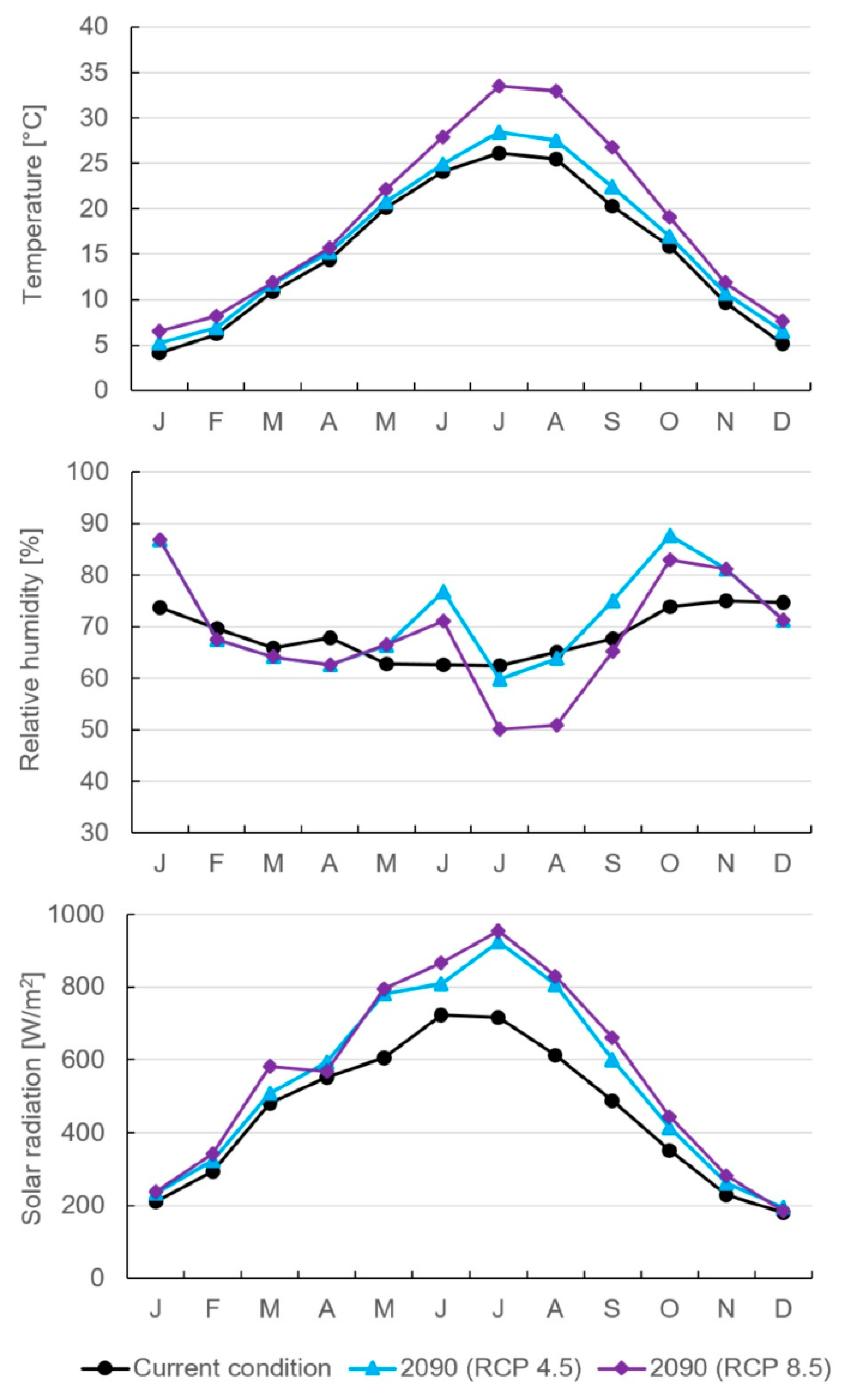
4.1. Future Climate Predicted for Milan

The comparison of the main environmental parameters (temperature, humidity, and solar radiation) of the two selected future scenarios with those of the current condition is shown below.

Regarding temperatures, the RCP 8.5 scenario reaches the highest values, with peaks in the summer months close to 44 °C, compared to 38 °C reached in the RCP 4.5 scenario (Figure 9). Similarly, for global solar radiation, an increase in all months of the year is expected in the future, with minimal differences in the winter and a consistent increase during summer.

Concerning relative humidity, in the two future scenarios, there are periods with high levels of RH in the winter and autumn, while the lowest values are found in the summer months; particularly hot and dry summers are expected in the future [19].

4.2. Future Risk Assessment

The possible future risks of deterioration that may occur to some of the main artworks of the Cathedral are hereafter analysed through the criteria described in Section 2.3.

4.2.1. Chemical Deterioration Risks

The risk of chemical deterioration concerns the yellowing of the varnish is shown below. In Figure 10, the hourly Lifetime Multiplier (LM) values calculated for the current condition and future scenarios related to the yellowing of varnish are shown.

Concerning the current condition, it can be noted that the period with higher risk (with LM below 0.75) is between May and October while considering the future scenarios this period is longer, from April to November, due to an early increase in temperatures.

To evaluate the average annual condition, the equivalent Lifetime Multiplier (eLM) has been calculated (Section 2.3.1); in

Table 7. Risk of chemical deterioration for different climate scenarios.

Scenario	eLM (Yellowing of Varnish)
Current condition	0.72
2090 (RCP 4.5)	0.56
2090 (RCP 8.5)	0.50

, the eLM values for the different scenarios are shown. In detail, regarding varnish deterioration in the current situation, the eLM is about 0.72, which represents a high-risk level. The situation in the next future is even more unfavourable, in fact, the eLM values are equal to 0.56 and 0.50, respectively, for RCP 4.5 and 8.5 scenarios. In particular, in the latter scenario, the eLM value of 0.50 indicates an expectation of durability of varnish is halved compared to the reference conditions (T = 20°C and RH = 50%).

4.2.2. Biological Deterioration Risks

Biological deterioration risks, analysed in this study, are induced by mould and insect attacks. The analysed surfaces are in the north walls of the Cathedral, which are characterised by the coldest temperatures and more probabilities of mould formation. In Figure 11, hourly surface temperature and relative humidity data, coloured according to the seasons, are reported for the current condition and for the two future scenarios.

As shown in Figure 11, scenarios RCP 4.5 and 8.5 are characterised by several periods with high values of relative humidity compared to the current condition. To verify the time in which spore germination occurs, the germination factor is calculated and reported below for the analysed scenarios.

According to Figure 12, in the current condition, there is a low risk related to mould growth. On the contrary, for RCP scenarios 4.5 and 8.5, there are different moments during the year in which the climatic conditions allow the spores to germinate for several consecutive days, particularly during July.

When spores germination starts, moulds will continue to grow at a speed that depends on microclimatic conditions. In this regard, Figure 13 shows the mycelium growth trend related to the three analysed scenarios.

In detail, it can be observed that for the recent scenario, the germination starts in March, while for the two future scenarios it starts two months earlier (about mid-January).

When the first germination occurs, the growth of mould is continuous and is particularly accelerated in July for both future scenarios.

The total annual growth for each scenario is shown in

Table 8. Annual mycelium growth for the different climate scenarios examined.

Scenario	Mycelial Growth/Year
Current condition	45
2090 (RCP 4.5)	146
2090 (RCP 8.5)	151

. These values correspond to a specific level of risk, as described in Section 2.3.2. In the current situation, the total annual growth is equal to 45 mm, which can be considered at low risk according to Table 3 (Section 2.3.2). Regarding the two future scenarios, the projection is similar. In particular, the total mould growth for scenario RCP 4.5 and 8.5 are 146 mm and 151 mm, respectively, hence, for the end of the XXI century, a medium risk of biological deterioration is expected.

Finally, insects can cause additional risk to organic materials, as shown in Figure 14, which represent a wooden bench of the Cathedral attacked by woodworms.

In Section 2.3.2, two categories of insects were analysed according to the favourable environmental conditions for their development. In detail, Category 1 includes insects like silverfish, psocopters, and woodworms, while Category 2 includes insects such as the drugstore beetle and the clothes moth.

In Figure 15, the distribution of the daily average relative temperature and humidity with the area of favourable conditions for the growth of the two categories is shown.

In

Table 9. Annual mycelium growth for the different climate scenarios examined.

Scenario	% Favourable Hours (Category 1)	% Favourable Hours (Category 2)
Current condition	15%	66%
2090 (RCP 4.5)	25%	58%
2090 (RCP 8.5)	22%	48%

, the percentages of favourable hours in a year for insect growth for the different scenarios are shown. For Category 1, the situation gets worst in the future; insect activity is expected to increase compared to the current condition of 10% and 7%, respectively, for RCP scenarios 4.5 and 8.5. For Category 2, on the other hand, there is an inverse trend due to the high temperatures reached especially in the summer months; the percentages of favourable hours for insect development compared to the current condition decrease by 8% and 18% for the RCP scenario 4.5 and 8.5, respectively.

4.2.3. Mechanical Deterioration Risks for Wooden Objects

The possible future risks of mechanical deterioration are analysed for two different wooden categories of objects, particularly numerous in the Duomo di Milano: panels and lacquered artefacts.

In Figure 16, the charts related to painted wooden panels are reported. As already described in Section 2.3.3, the safety area to avoid mechanical damage in the material is coloured green.

For the current condition, the months with the highest risk are March and May, which are characterised by high levels of RH; therefore, in Figure 16, the response RH curve exceeds the safety area, with possible negative effects on the wooden panels. For both future scenarios, the behaviour is similar: in January and June characterised by a continuous number of days with high RH (possibly due to very intense rainfall events), higher deformations are produced due to the rapid response to the moisture of the panel surface, while the whole panel adapts more slowly. Compared to the current period, in the future scenarios, there are moments when the response RH curve exceeds the green area at the bottom; these moments are in correspondence of sudden drops in relative humidity. For example, in the first days of July for the 2090 scenario (RCP 8.5), the external relative humidity changes from about 85% to 15% in less than 24 h, which leads to a very low RH response of the surface layer of the panels after just four days, while the response RH of the entire panel is stable on intermediate values. These excessive deformations result in both swelling and shrinkage of the surface layer of the panel and can cause cracks to appear in the wooden panel, with a probability that increases based on the number of times and the intensity of exceedance in the green area.

Finally, the possible risk of mechanical damage to lacquered wood artefacts is analysed, as illustrated in Figure 17.

About wooden artefacts such as confessionals, furniture, etc., it is evident from Figure 17 that neither in the recent nor the future situation, risks of mechanical degradation are expected. This positive behaviour is due to the protective lacquer in the wooden elements, which considerably slows down the absorption of environmental humidity (the response time for the whole object is estimated to be about 40 days, for further details see Section 2.3.3). However, it should be mentioned that the response time can decrease dramatically if the object is already damaged, as shown in Figure 18 of the confessional.

4.2.4. Mechanical Deterioration Risks in Masonry

Finally, the last risk of deterioration analysed is caused by salts present in the masonry. Figure 19. shows the times when the critical RH value is exceeded for Halite deliquescence and the phase transition of Thénardite to Mirabilite. In this study, the surfaces analysed are those in the south walls of the Cathedral, where some efflorescence problems have been detected [67].

As described in Section 2.3.4, to evaluate the number of crystallization cycles of the salts and to assess the related risks, it is necessary to consider the daily average T_s and RH. In

Table 10. Deliquescence-crystallization cycles (Halite) and phase transitions (Thénardite to Mirabilite) of the two salts analysed for the different climate scenarios.

Scenario	N° Cycles/Year (Halite)	N° Cycles/Year (Thénardite-Mirabilite)
Current condition	19	26
2090 (RCP 4.5)	16	22
2090 (RCP 8.5)	18	23

, the number of cycles per year estimated for each scenario analysed is reported. Compared to the current condition, in the future, a worsening is not expected, as can be seen from Table 10, where the number of cycles is always lower than that related to the present condition, for both types of salts.

5. Conclusions

Heritage buildings and the precious artworks contained therein, represent inestimable cultural and artistic evidence from the past and contribute to providing a sense of identity for people. Such heritage may be particularly threatened in the near future by the effects of climate change.

In that respect, the present work described a method that combines on-site measurements and computer simulation to make projections of the future indoor climate of heritage buildings and analyse possibles risks for artworks conservation using risk assessment criteria based on three main categories of deterioration risk: chemical, biological, and mechanical. The method proposed in this paper can be adopted by other researchers, practitioners, architects, etc., involved in the evaluation of the risks caused by future climate change projections.

The presented method has been applied to one of the most important heritage buildings in Italy, which is characterised by a particularly huge volume and high-massive envelope.

The main results of this study are summarized here and in

Table A1. Summary of climate change effects on different material deterioration risks.

	Chemical Deterioration Risk	Biological Deterioration Risks			Mechanical Deterioration Risks
Causes of deterioration	Acceleration of chemical reactions	Mould	Insects (category 1)	Insects (category 2)	Rapid climate variations	Rapid climate variations	Salts (Halite)	Salts (Thénardite to Mirabilite)
Material interested	Varnish of paintings	Several materials	Wood, paper, other organic materials	Clothes, other organic materials	Wooden panels	Wooden furniture	Masonry, stone sculptures	Masonry, stone sculptures
Current condition
	Unfavourable conditions for material conservation	Low risk	Possible risks of insect attack	Conditions of high risk of insect attack	Possible elastic deformation phenomena (compression events)	Low risk. Caution with already deteriorated objects	Low risk	Low risk
2090 (RCP 4.5)
	A 22% increase in risk is expected with respect to the current condition	Increased risk compared to the current condition, possible mould-related problems	A 10% increase in risk is expected with respect to the current condition	An 8% decrease in risk is expected with respect to the current condition	Increased risk is expected, elastic strain threshold exceeded (compression and tension events)	The risk increase. Caution with already deteriorated objects	Low risk	Low risk
2090 (RCP 4.5)
	A 31% increase in risk is expected with respect to the current condition	Further increase in risk, possible mould-related problems	A 7% increase in risk is expected with respect to the current condition	An 18% decrease in risk is expected with respect to the current condition	A further increase in risk is expected, exceeding the elastic deformation threshold (compression and tension events)	The risks further increase. Caution with already deteriorated objects	Low risk	Low risk

(Appendix A):

• Regarding the risk of chemical deterioration of the protective varnish layer in paintings, it appears that the current conditions are not favourable for proper conservation. In the two future scenarios, the situation gets even worse in a quite similar way;
• The risk of biological deterioration due to mould will increase in the future due to a prolonged period with high indoor relative humidity. The projected mould growth for the RCP 4.5 and 8.5 scenarios are similar;
• The risk of biological deterioration caused by insects is different for Category 1 and Category 2. For the first category of insects, an increase of favourable conditions to their growth is predicted for both future scenarios. For the second category, the unfavourable conditions of the present will decrease in the future, due to excessive increase in temperatures; however, the risk associated remains high;
• The risk of mechanical damage in painted wooden panels will be higher in the future. In the two forecasted climate scenarios, there are events in which the low relative humidity reached during summer (very hot and dry) could generate an excessive shrinkage of the surface layer of the panels with possible crack formation. In the RCP 8.5 scenario, this situation is further intensified;
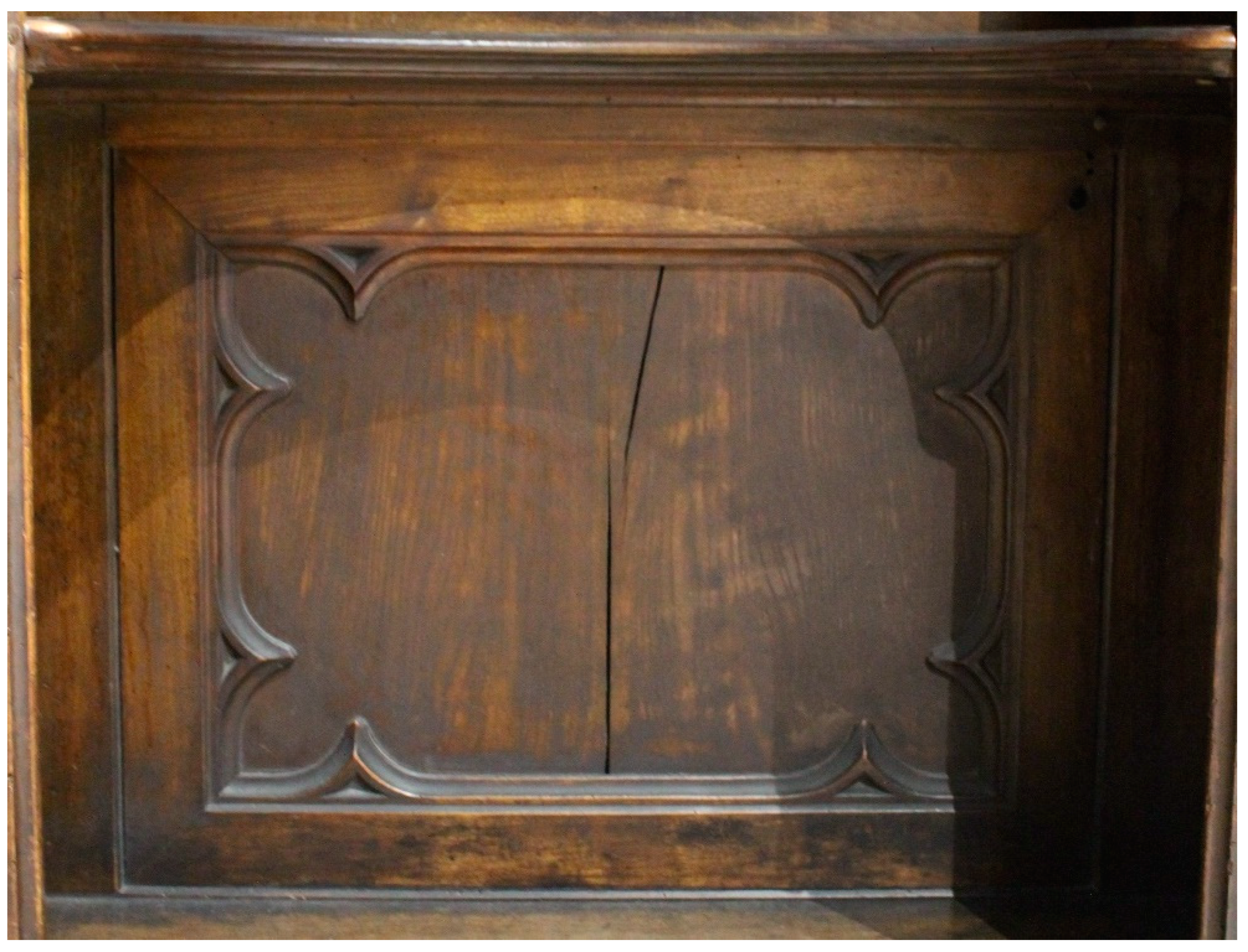
• With regards to wooden furniture, the deformations generated by climatic variations in the present and future do not appear risky. However, for already damaged objects the increased risk of deterioration cannot be excluded;
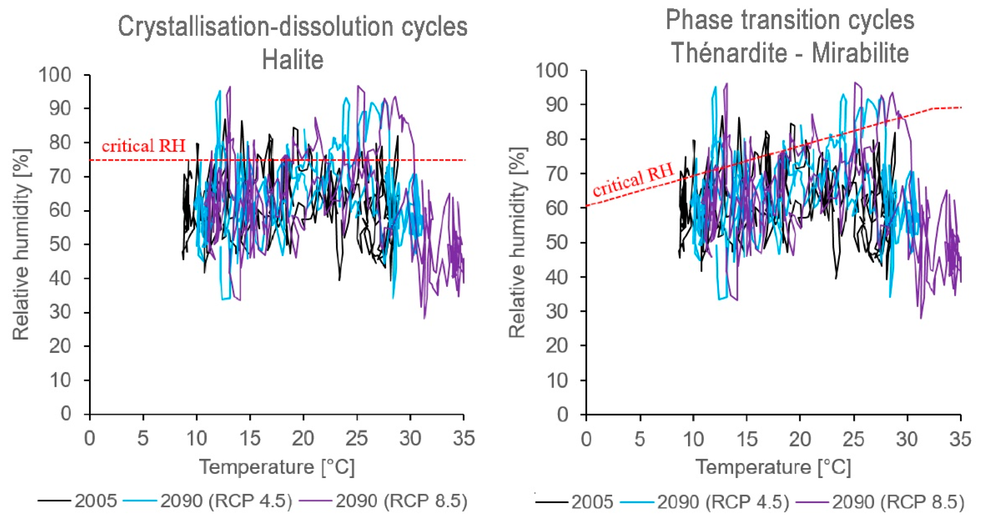
• The risks of deterioration in stone structures generated by the two types of salts analysed do not increase in any of the future scenarios considered.

In conclusion, for some artworks, the number of adverse events appears not to be increasing with respect to the current condition, while for others the risk of deterioration is expected to increase substantially, with more intensity in the scenario RCP 8.5. The results of this study help to understand how the future climate could influence the indoor environment in huge masonry buildings and allow planning possible targeted mitigation strategies aimed to reduce the future risks for heritage conservation.

Such strategies/solutions can be both active or passive. However, in several historic buildings, like the Duomo di Milano, passive strategies are preferable due to the constraints which they are subjected to; some examples of passive solutions to improve the indoor environmental conditions can be the control of the natural ventilation through the openings management, integrated pest management (IPM), the management of the visitors, etc. While regarding the adoption of active solutions, localized HVAC systems or fans can be installed, if possible, to increase the air exchanges with the outdoor during particular conditions, etc. Moreover, if the conservation conditions become too unfavourable for the preservation of the artworks, the movable objects can be relocated to a safer location.

In this study, the projections made can be useful as information of possible future risks for the building and artworks, allowing the authorities to be more conscious and prepared to plan suitable and timely interventions. Future development of this research can be the implementation of the simulation model to evaluate hygrothermal stratifications in huge volume buildings and the definition of a long-term protocol to mitigate the negative effects of future climate on the conservation of the materials of the Duomo di Milano.

References

1. Gandini, A.; Garmendia, L.; San Mateos, R. Towards sustainable historic cities: Adaptation to climate change risks. Entrep. Sustain. Issues 2017, 4, 319–327. [Google Scholar] [CrossRef] [Green Version]
2. Leissner, J.; Kilian, R.; Kotova, L.; Jacob, D.; Mikolajewicz, U.; Broström, T.; Ashley-Smith, J.; Schellen, H.L.; Martens, M.; Van Schijndel, J.; et al. Climate for culture: Assessing the impact of climate change on the future indoor climate in historic buildings using simulations. Herit. Sci. 2015, 3, 1–15. [Google Scholar] [CrossRef]
3. Muñoz González, C.M.; León Rodríguez, A.L.; Suárez Medina, R.; Jaramillo, J.R. Effects of future climate change on the preservation of artworks, thermal comfort and energy consumption in historic buildings. Appl. Energy 2020, 276, 1–12. [Google Scholar] [CrossRef]
4. Antretter, F.; Schöpfer, T.; Kilian, R. An approach to assess future climate change effects on indoor climate of a historic stone church. In Proceedings of the 9th Nordic Symposium on Building Physics; Fraunhofer-Institut Für Bauphysik, Holzkirchen, Germany, 29 May–2 June 2011; Volume 2, pp. 849–856. [Google Scholar]
5. Sesana, E.; Gagnon, A.S.; Bertolin, C.; Hughes, J. Adapting cultural heritage to climate change risks: Perspectives of cultural heritage experts in europe. Geosciences 2018, 8, 305. [Google Scholar] [CrossRef] [Green Version]
6. Coelho, G.B.A.; Silva, H.E.; Henriques, F.M.A. Impact of climate change in cultural heritage: From energy consumption to artefacts’ conservation and building rehabilitation. Energy Build. 2020, 224, 110250. [Google Scholar] [CrossRef]
7. Sesana, E.; Gagnon, A.S.; Ciantelli, C.; Cassar, J.A.; Hughes, J.J. Climate change impacts on cultural heritage: A literature review. Wiley Interdiscip. Rev. Clim. Chang. 2021, 12, 1–29. [Google Scholar] [CrossRef]
8. Ciantelli, C.; Palazzi, E.; Von Hardenberg, J.; Vaccaro, C.; Tittarelli, F.; Bonazza, A. How can climate change affect the UNESCO cultural heritage sites in panama? Geosciences 2018, 8, 296. [Google Scholar] [CrossRef] [Green Version]
9. Carroll, P.; Aarrevaara, E. Review of potential risk factors of cultural heritage sites and initial modelling for adaptation to climate change. Geosciences 2018, 8, 322. [Google Scholar] [CrossRef]
10. Bertolin, C. Preservation of cultural heritage and resources threatened by climate change. Geosciences 2019, 9, 250. [Google Scholar] [CrossRef] [Green Version]
11. Haugen, A.; Bertolin, C.; Leijonhufvud, G.; Olstad, T.; Broström, T. A methodology for long-term monitoring of climate change impacts on historic buildings. Geosciences 2018, 8, 370. [Google Scholar] [CrossRef] [Green Version]
12. Anaf, W.; Leyva Pernia, D.; Schalm, O. Standardized indoor air quality assessments as a tool to prepare heritage guardians for changing preservation conditions due to climate change. Geosciences 2018, 8, 276. [Google Scholar] [CrossRef] [Green Version]
13. Loli, A.; Bertolin, C. Indoor multi-risk scenarios of climate change effects on building materials in scandinavian countries. Geosciences 2018, 8, 347. [Google Scholar] [CrossRef] [Green Version]
14. Melin, C.B.; Hagentoft, C.E.; Holl, K.; Nik, V.M.; Kilian, R. Simulations of moisture gradients in wood subjected to changes in relative humidity and temperature due to climate change. Geosciences 2018, 8, 378. [Google Scholar] [CrossRef] [Green Version]
15. Menéndez, B. Estimators of the impact of climate change in salt weathering of cultural heritage. Geosciences 2018, 8, 401. [Google Scholar] [CrossRef] [Green Version]
16. Sabbioni, C.; Cassar, M.; Brimblecombe, P.; Lefevre, R.A. Vulnerability of cultural heritage to climate change. Pollut. Atmos. 2009, 157–169. [Google Scholar]
17. NOAHS ARK (Global Climate Change Impact on Built Heritage and Cultural Landscapes). Available online: https://cordis.europa.eu/project/id/501837/reporting/it (accessed on 21 April 2021).
18. European Project Climate for Culture. Available online: https://www.climateforculture.eu/ (accessed on 5 January 2021).
19. Castellari, S.; Venturini, S.; Ballarin Denti, A.; Bigano, A.; Bindi, M.; Bosello, F.; Carrera, L.; Chiriaco, M.V.; Danovaro, R.; Desiato, F.; et al. Rapporto Sullo Stato Delle Conoscenze Scientifiche su Impatti, Vulnerabilità ed Adattamento ai Cambiamenti Climatici in Italia; Ministero dell’Ambiente e della Tutela del Territorio e del Mare: Rome, Italy, 2014. [Google Scholar]
20. Lankester, P.; Brimblecombe, P. The impact of future climate on historic interiors. Sci. Total Environ. 2012, 417, 248–254. [Google Scholar] [CrossRef] [PubMed]
21. Lankester, P.; Brimblecombe, P. Future thermohygrometric climate within historic houses. J. Cult. Herit. 2012, 13, 1–6. [Google Scholar] [CrossRef]
22. Brimblecombe, P.; Lankester, P. Long-term changes in climate and insect damage in historic houses. Stud. Conserv. 2013, 58, 13–22. [Google Scholar] [CrossRef]
23. Camuffo, D.; Bertolin, C.; Bonazzi, A.; Campana, F.; Merlo, C. Past, present and future effects of climate change on a wooden inlay bookcase cabinet: A new methodology inspired by the novel European Standard EN 15757:2010. J. Cult. Herit. 2014, 15, 26–35. [Google Scholar] [CrossRef]
24. ENSEMBLES Project. Available online: https://www.ensembles-eu.org/ (accessed on 18 May 2021).
25. Jacob, D.; Elizalde, A.; Haensler, A.; Hagemann, S.; Kumar, P.; Podzun, R.; Rechid, D.; Remedio, A.R.; Saeed, F.; Sieck, K.; et al. Assessing the transferability of the regional climate model REMO to different coordinated regional climate downscaling experiment (CORDEX) regions. Atmosphere 2012, 3, 181–199. [Google Scholar] [CrossRef] [Green Version]
26. University of Southampton. CCWorldWeatherGen. Available online: https://energy.soton.ac.uk/climate-change-world-weather-file-generator-for-world-wide-weather-data-ccworldweathergen/ (accessed on 21 August 2021).
27. Intergovernmental Panel on Climate Change (IPCC). Climate Change 2014 Synthesis Report; Intergovernmental Panel on Climate Change (IPCC): Geneva, Switzerland, 2014. [Google Scholar]
28. Pretelli, M.; Fabbri, K. (Eds.) Historic Indoor Microclimate of the Heritage Buildings; Springer: Berlin/Heidelberg, Germany, 2018; ISBN 9783319603414. [Google Scholar]
29. Huerto-Cardenas, H.E. Validation of Historical Buildings Energy Models: A Method Based on Microclimatic Control Parameters. Ph.D. Thesis, Politecnico di Milano, Milano, Italy, 25 March 2020. [Google Scholar]
30. Miglioli, A.; Huerto-Cardenas, H.; Leonforte, F.; Aste, N.; Del Pero, C. Energy and economic assessment of HVAC solutions for the armoury hall at the Palazzo Ducale in Mantua. Procedia Struct. Integr. 2020, 29, 118–125. [Google Scholar] [CrossRef]
31. Akkurt, G.G.; Aste, N.; Borderon, J.; Buda, A.; Calzolari, M.; Chung, D.; Costanzo, V.; Del Pero, C.; Evola, G.; Huerto-Cardenas, H.E.; et al. Dynamic thermal and hygrometric simulation of historical buildings: Critical factors and possible solutions. Renew. Sustain. Energy Rev. 2020, 118, 109509. [Google Scholar] [CrossRef]
32. Huerto-Cardenas, H.E.; Leonforte, F.; Aste, N.; Del Pero, C.; Evola, G.; Costanzo, V.; Lucchi, E. Validation of dynamic hygrothermal simulation models for historical buildings: State of the art, research challenges and recommendations. Build. Environ. 2020, 180, 107081. [Google Scholar] [CrossRef]
33. American Society of Heating, Refrigerating and Air-Conditioning Engineers, Inc. ASHRAE Guideline 14-2002 Measurement of Energy and Demand Savings; American Society of Heating, Refrigerating and Air-Conditioning Engineers, Inc.: Peachtree Corners, GA, USA, 2002; p. 170. [Google Scholar]
34. Federal Energy Management Program. FEMP M&V Guidelines: Measurement and Verification for Federal Energy Projects-Version 3.0; Federal Energy Management Program: Washington, DC, USA, 2008. [Google Scholar]
35. International Performance Measurement & Verification Protocol Committee. Efficiency Valuation Organization International Performance Measurement and Verification Protocol: Concepts and Options for Determining Energy and Water Savings Volume 1; International Performance Measurement & Verification Protocol Committee: Washington, DC, USA, 2012; Volume 1. [Google Scholar]
36. Moazami, A.; Nik, V.M.; Carlucci, S.; Geving, S. Impacts of future weather data typology on building energy performance—Investigating long-term patterns of climate change and extreme weather conditions. Appl. Energy 2019, 238, 696–720. [Google Scholar] [CrossRef]
37. Meteotest Meteonorm. Available online: https://meteonorm.com/en/meteonorm-version-8 (accessed on 20 January 2004).
38. ARUP. Argos Analytics LLC Weathershift. Available online: https://www.weathershift.com/heat (accessed on 9 January 2021).
39. Martens, M.H.J. Climate Risk Assessment in Museums: Degradation Risks Determined from Temperature and Relative Humidity Data. Ph.D. Thesis, Technische Universiteit Eindhoven, Eindhoven, The Netherlands, 2012. [Google Scholar]
40. Silva, H.E.; Henriques, F.M.A.; Henriques, T.A.S.; Coelho, G. A sequential process to assess and optimize the indoor climate in museums. Build. Environ. 2016, 104, 21–34. [Google Scholar] [CrossRef]
41. Huijbregts, Z.; Kramer, R.P.; Martens, M.H.J.; van Schijndel, A.W.M.; Schellen, H.L. A proposed method to assess the damage risk of future climate change to museum objects in historic buildings. Build. Environ. 2012, 55, 43–56. [Google Scholar] [CrossRef]
42. Corgnati, S.P.; Fabi, V.; Filippi, M. A methodology for microclimatic quality evaluation in museums: Application to a temporary exhibit. Build. Environ. 2008, 44, 1253–1260. [Google Scholar] [CrossRef]
43. Fabbri, K.; Bonora, A. Two new indices for preventive conservation of the cultural heritage: Predicted risk of damage and heritage microclimate risk. J. Cult. Herit. 2021, 47, 208–217. [Google Scholar] [CrossRef]
44. Ente nazionale italiano di unificazione. UNI 10829: Luglio 1999—BENI di Interesse Storico e Artistico—Condizioni Ambientali di Conservazione—Misurazione ed Analisi; Ente Nazionale Italiano di Unificazione: Rome, Italy, 1999; p. 24. [Google Scholar]
45. MIBAC (Italian Ministry of Cultural Heritage). Atto di Indirizzo Sui Criteri Tecnico-Scientifi ci e Sugli Standard di Funzionamento e Sviluppo Dei Musei, Ambito VI. D.Lgs. 112/1998 (Art. 150, Comma 6); Technical Report; Italian Law: Rome, Italy, 2001; pp. 81–94. [Google Scholar]
46. European Committee for Standardization. CEN EN 15757: 2010—Conservation of Cultural Property. Specifications for Temperature and Relative Humidity to Limit Climate-Induced Mechanical Damage in Organic Hygroscopic Materials; European Committee for Standardization: Brussels, Belgium, 2010; p. 18. [Google Scholar]
47. American Society of Heating, Refrigerating and Air-Conditioning Engineers, Inc. ASHRAE Energy Guideline for Historical Buildings, ASHRAE 34P, Standards Michigan; American Society of Heating, Refrigerating and Air-Conditioning Engineers, Inc.: Peachtree Corners, GA, USA, 2019. [Google Scholar]
48. Michalski, S. Double the Life for Each Five-Degree Drop, More Than Double the Life for Each Halving of Relative Humidity. In Proceedings of the Thirteenth Triennial Meeting ICOM-CC, Rio de Janeiro, Brazil, 22–27 September 2002; Volume I, pp. 66–72. [Google Scholar]
49. Silva, H.E.; Henriques, F.M.A. Preventive conservation of historic buildings in temperate climates. The importance of a risk-based analysis on the decision-making process. Energy Build. 2015, 107, 26–36. [Google Scholar] [CrossRef]
50. Verticchio, E.; Frasca, F.; Garcìa-Diego, F.J.; Siani, A.M. Investigation on the use of passive microclimate frames in view of the climate change scenario. Climate 2019, 7, 98. [Google Scholar] [CrossRef] [Green Version]
51. Sedlbauer, K. Prediction of Mould Fungus Formation on the Surface of and Inside Buildings Components. Ph.D. Thesis, Fraunhofer Institute for Building Physics, Stuttgart, Germany, 2001. [Google Scholar]
52. Vereecken, E.; Roels, S. Review of mould prediction models and their influence on mould risk evaluation. Build. Environ. 2012, 51, 296–310. [Google Scholar] [CrossRef] [Green Version]
53. Krus, M.; Sedlbauer, K. A new model for prediction and its application in practice. In Proceedings of the 6th International Conference on Indoor Air Quality, Ventilation & Energy Conservation in Buildings IAQVEC 2007, Sendai, Japan, 28–31 October 2007. [Google Scholar]
54. Vereecken, E.; Saelens, D.; Roels, S. A comparison of different mould prediction models. In Proceedings of the 12th Conference of International Building Performance Simulation Association, Sydney, NSW, Australia, 14–16 November 2011; Volume 6, pp. 1934–1941. [Google Scholar]
55. Strang, T.J.K. Studies in Pest Control for Cultural Property. Ph.D. Thesis, University of Gothenburg, Gothenburg, Sweden, 2012. ISBN 9789173467346. [Google Scholar]
56. Vici, P.D.; Mazzanti, P.; Uzielli, L. Mechanical response of wooden boards subjected to humidity step variations: Climatic chamber measurements and fitted mathematical models. J. Cult. Herit. 2006, 7, 37–48. [Google Scholar] [CrossRef]
57. Bratasz, Ł.; Kozłowski, R.; Kozłowska, A.; Rivers, S.; Kozlowski, R.; Kozlowska, A. Conservation of the Mazarin Chest: Structural response of Japanese lacquer to variations in relative humidity. In Proceedings of the ICOM-CC Triennial Meeting, New Delhi, India, 22–26 September 2008; Volume 2, pp. 1086–1093. [Google Scholar]
58. Mecklenburg, M.F.; Tumosa, C.S.; Erhardt, D. Structural response of painted wood surfaces to changes in ambient relative humidity. In Painted Wood: History and Conservation; Dorge, V., Howlett, F.C., Eds.; The Getty Conservation Institute: Los Angeles, CA, USA, 1998; pp. 464–483. [Google Scholar]
59. Camuffo, D. Microclimate for Cultural Heritage: Conservation and Restoration of Indoor and Outdoor Monuments; Elsevier: Amsterdam, The Netherlands, 2013; ISBN 9780444632968. [Google Scholar]
60. Grossi, C.M.; Brimblecombe, P.; Menéndez, B.; Benavente, D.; Harris, I.; Déqué, M. Climatology of salt transitions and implications for stone weathering. Sci. Total Environ. 2011, 409, 2577–2585. [Google Scholar] [CrossRef]
61. Sabbioni, C.; Brimblecombe, P.; Cassar, M. The Atlas of Climate Change Impact on European Cultural Heritage: Scientific Analysis and Management Strategies; Anthem Press: London, UK, 2010; ISBN 9781843313953. [Google Scholar]
62. Varas-Muriel, M.J.; Fort, R. Microclimatic monitoring in an historic church fitted with modern heating: Implications for the preventive conservation of its cultural heritage. Build. Environ. 2018, 145, 290–307. [Google Scholar] [CrossRef]
63. D’Agostino, V.; Alfano, F.R.D.; Palella, B.I.; Riccio, G. The museum environment: A protocol for evaluation of microclimatic conditions. Energy Build. 2015, 95, 124–129. [Google Scholar] [CrossRef]
64. Cardinale, T.; Rospi, G.; Cardinale, N. The influence of indoor microclimate on thermal comfort and conservation of artworks: The case study of the Cathedral of Matera (South Italy). Energy Procedia 2014, 59, 425–432. [Google Scholar] [CrossRef] [Green Version]
65. Silva, H.E.; Henriques, F.M.A. Microclimatic analysis of historic buildings: A new methodology for temperate climates. Build. Environ. 2014, 82, 381–387. [Google Scholar] [CrossRef]
66. Muñoz-González, C.M.; León-Rodríguez, A.L.; Navarro-Casas, J. Air conditioning and passive environmental techniques in historic churches in Mediterranean climate. A proposed method to assess damage risk and thermal comfort pre-intervention, simulation-based. Energy Build. 2016, 130, 567–577. [Google Scholar] [CrossRef]
67. Aste, N.; Adhikari, R.S.; Buzzetti, M.; Torre, S.D.; Del Pero, C.; Huerto, C.H.E.; Leonforte, F. Microclimatic monitoring of the Duomo (Milan Cathedral): Risks-based analysis for the conservation of its cultural heritage. Build. Environ. 2019, 148, 240–257. [Google Scholar] [CrossRef]
68. Costanzo, V.; Fabbri, K.; Schito, E.; Petrelli, M.; Marletta, L. Microclimate monitoring and conservation issues of a Baroque church in Italy: A risk assessment analysis. Build. Res. Inf. 2021, 1–19. [Google Scholar] [CrossRef]
69. Frasca, F.; Verticchio, E.; Cornaro, C.; Siani, A.M. Performance assessment of hygrothermal modelling for diagnostics and conservation in an Italian historical church. Build. Environ. 2021, 193, 107672. [Google Scholar] [CrossRef]
70. EnergyPlus (Version 8.9). Available online: https://energyplus.net/downloads (accessed on 21 August 2021).
71. EnergyPlus Documentation—Engineering Reference. Available online: https://energyplus.net/documentation (accessed on 21 August 2021).
72. Lee, K.O.; Medina, M.A.; Sun, X. Development and verification of an EnergyPlus-based algorithm to predict heat transfer through building walls integrated with phase change materials. J. Build. Phys. 2016, 40, 77–95. [Google Scholar] [CrossRef] [Green Version]
73. Giudice, G.M.L.; Buratti, C.; Baldinelli, G. Indagini Spettrofotometriche sulle proprieta’ di trasparenza e riflessione delle vetrate antiche decorate con tecniche superficiali. In Proceedings of the Congr. Naz. AIDI 2002; 2002; pp. 1–8. Available online: www.ciriaf.it/ft/File/Pubblicazioni/pdf/950.pdf (accessed on 17 January 2021).
74. Huerto-Cardenas, H.E.; Leonforte, F.; Del Pero, C.; Aste, N.; Buzzetti, M.; Adhikari, R.S.; Miglioli, A. Impact of moisture buffering effect in the calibration of historical buildings energy models: A case study. J. Sustain. Dev. Energy, Water Environ. Syst. 2020. [Google Scholar] [CrossRef]
75. La Repubblica, Il Duomo di Milano Resta Deserto: Senza Turisti, 90% di Visitatori in Meno. Available online: https://milano.repubblica.it/cronaca/2020/07/01/news/il_duomo_di_milano_resta_deserto_senza_turisti_90_di_visitatori_in_meno-260655353/ (accessed on 21 August 2021).
76. ARPA, Richiesta Dati Misurati. Available online: https://www.arpalombardia.it/Pages/Meteorologia/Richiesta-dati-misurati.aspx (accessed on 17 January 2021).
77. Erco, Far Percepire le Dimensioni Maestose: La Nuova Illuminazione del Duomo di Milano. Available online: https://www.erco.com/it/progetti/zoom/reportage/duomo-di-milano-6168/ (accessed on 21 August 2021).
78. Coakley, D.; Raftery, P.; Keane, M. A review of methods to match building energy simulation models to measured data. Renew. Sustain. Energy Rev. 2014, 37, 123–141. [Google Scholar] [CrossRef] [Green Version]
Figure 1. Phases of the adopted method.
Climate 09 00132 g001
Figure 2. Isolines of spore germination and mould growth for the different categories of substrate. Red areas represent T and RH conditions at risk for spore germination and mycelial growth; the colour intensity indicates higher risk. Adapted from [51].
Climate 09 00132 g002
Figure 3. Mechanical risk assessment for the wooden support of paintings. The green, orange and red areas indicate conditions with a low, medium and high risk of deterioration respectively. Adapted from [58].
Climate 09 00132 g003
Figure 4. Mechanical risk assessment for lacquered wood furniture. The green and orange areas indicate conditions with a low and medium risk of deterioration respectively. Adapted from [57].
Climate 09 00132 g004
Figure 5. Some of the artworks of the Duomo di Milano. (1,2) shows stone sculptures; (3,4) shows various artefacts located in altars of the aisles; (5) shows one of the organ cases which has large wooden panels painted; (6) shows a bronze candelabrum with a marble base; (7) shows a pulpit made with bronze caryatids and balcony with gilded copper balusters; (8) shows a wooden confessional.
Climate 09 00132 g005
Figure 6. View of the thermal zones of the simulation model.
Climate 09 00132 g006
Figure 7. Estimation of time elapsed between peak outdoor (MR outdoor) and indoor (MR indoor) mixing ratio for some sample days of 2019 and 2020 for the first and the second operating condition.
Climate 09 00132 g007
Figure 8. Comparative graphs between measured and simulated temperature data.
Climate 09 00132 g008
Figure 9. Mean monthly temperature, relative humidity, and solar radiation for the different climate scenarios.
Climate 09 00132 g009
Figure 10. Evaluation of the deterioration of the protective varnish of paintings (yellowing). LM trend for the different scenarios analysed.
Climate 09 00132 g010
Figure 11. Ts-RH hourly data concerning the mould germination isolines for the analysed scenarios.
Climate 09 00132 g011
Figure 12. Germination factor for the analysed scenarios.
Climate 09 00132 g012
Figure 13. Mould growth for the different scenarios analysed.
Climate 09 00132 g013
Figure 14. View of a wooden bench attacked by woodworm.
Climate 09 00132 g014
Figure 15. Distribution of daily mean T and RH for the different scenarios analysed, for the favourable conditions for insect growth. The picture on the (left) shows the optimal conditions for insects belonging to Category 1 and the picture on the (right) those for Category 2.
Climate 09 00132 g015
Figure 16. Risks associated with mechanical deterioration on painted wood panels for climate change scenarios.
Climate 09 00132 g016
Figure 17. Risks associated with mechanical deterioration on lacquered wood furniture for climate change scenarios.
Climate 09 00132 g017
Figure 18. Confessional with already ongoing deterioration process.
Climate 09 00132 g018
Figure 19. Ts and RH daily profile versus critical RH for Halite deliquescence (left) and Thénardite to Mirabilite phase transition (right) for the different scenarios analysed.
Climate 09 00132 g019