
A Decomposition-Based Multi-Objective Evolutionary Algorithm for Solving Low-Carbon Scheduling of Ship Segment Painting

Abstract
:1. Introduction
- At this stage, ship enterprises are facing green transformation, and a ship segmental painting low-carbon scheduling model is established for the ship segmental painting low-carbon scheduling during the operation of the painting team during the ship segmental painting process, which is characterized by the problems of low efficiency and excessive carbon emission;
- An MD/ABC algorithm is proposed for solving the above model.
- (1)
- Designing a two-level coding method for ship segmental painting low-carbon scheduling model;
- (2)
- Designing five neighborhood switching methods to ensure that the subproblems can be fully optimized and enhance the global exploration performance of the algorithm;
- (3)
- Improving the competition mechanism by using TOPSIS technology and introducing an angle strategy to further enhance the local search capability of the algorithm;
- (4)
- Designing an exchange strategy for the solutions of subproblems in different neighborhoods to further enhance the performance of the algorithm.
2. Modeling of Low-Carbon Scheduling Problem for Ship Segment Painting
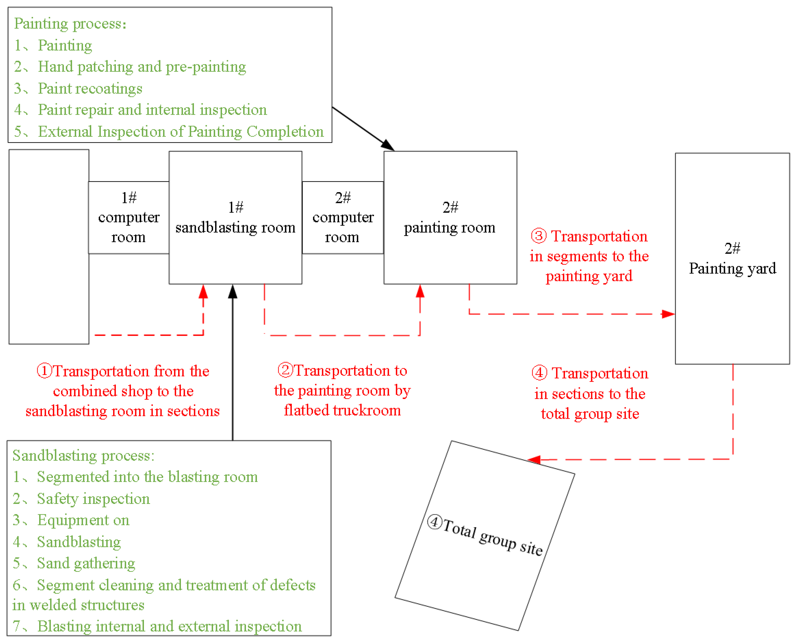
2.1. Segmental Painting Process
- Segmentation into the sandblasting room: Large flatbed trucks are used to transport the sand to be blasted into the sandblasting room in segments and close the flexible door of the room;
- Safety inspection: It is performed mainly using manual methods, the comprehensive inspection of scaffolding, etc., to ensure the safety of construction personnel and inspection of construction tools and labor protection supplies;
- Equipment: It mainly includes indoor lighting, a whole room dust removal system, a dehumidification system, and a sandblasting system;
- Sandblasting operation: A sandblasting gun is used to treat the segments and remove the oxidized skin and other impurities on the surface of the steel plate to make it show metallic luster. At the same time, sufficient lighting is ensured to guarantee the safety of the operating personnel, and equipment such as dust removal and dehumidification are activated to control the temperature and humidity of the air and the concentration of dust in the plant;
- Sand collecting operation: At present, manual sand collecting and vacuum sand sucking machines are used in combination. The vacuum sand-sucking machine consumes a lot of electricity when used, and at the same time, it needs the whole room’s dust removal equipment, dehumidifier, and other equipment to cooperate;
- Sectional cleaning and welding structural defects: They are performed mainly through manual pneumatic tools to remove welding spatters, free-cutting edges, running holes, and other structural defects, as well as residual dust on the surface of the steel plate. In order to meet the requirements and improve the quality of subsequent painting construction, it is necessary to cooperate with the whole room dust removal, dehumidifier and other equipment;
- Blasting internal and external inspection: After completing the sand blasting treatment, the segments need to be transported by flatbed trucks to the painting plant for inspection.
- Spraying construction: The process of manually spraying paint on the surface of steel plates utilizing high-pressure airless spray pumps. The construction requires a small amount of compressed air, and dehumidifiers and organic solvent purification devices are enabled in the plant to ensure that harmful gases, such as VOC, are fully absorbed and environmentally friendly emissions are realized;
- Manual repair and pre-coating: The process of repairing areas that could not be effectively sprayed or were missed during the spraying process, usually by hand brushing or roller coating;
- Paint recoating: Recoating is performed using manual airless spraying construction;
- Paint repair and internal inspection: The film thickness test and the malpractice inspection of completed paint are employed to eliminate problems and ensure that the film-forming effect after construction meets the process requirements;
- External inspection of paint completion: It is performed mainly by the shipowner, paint service provider, crew construction personnel, etc., according to the construction process specifications and quality standards, etc., on the construction of the end of the segment for the external inspection of the film formation situation.
2.2. Description of the Problem
- Each segment must pass through all phases sequentially, with each segment job assigned to a transportation device at a given phase;
- At any given time, a maximum of one segmental painting team may be processed, and a maximum of one segment may be processed on one painting team;
- Interruptions and preemption are not permitted;
- Sections are transported to the paint shop immediately after completion in the sandblasting shop;
- The buffer between the stages of the segmented painting workshop is unrestricted;
- The types of equipment turn on when the paint team is assigned the first segment to begin processing. Only when all segments of the paint team are completed do the types of equipment turn off;
- Segmented jobs must be completely processed by the painting team in the last stage before the next stage can be started;
- Paint teams are permitted idle time, and segments are not to be processed by the paint team until the adjacent operation has been adjusted;
2.3. Carbon Emission Category Analysis
- Manufacturing carbon emissions. Manufacturing carbon emissions represent the carbon emissions emitted by equipment within ship painting workshops during the operation. The overall manufacturing carbon emissions can be calculated as CW in Equation (1).
- Adjustment of carbon emissions. Adjustment carbon emission refers to the carbon emission generated during the adjustment time required for the workshop equipment to process different segments successively. The total carbon emission under adjustment is calculated as CS shown in Equation (2).
- Idle carbon emissions. Idle carbon emission refers to the carbon emission generated by the idle state of workshop equipment, and the total carbon emission under the idle state is calculated as CI shown in Equation (3).
- Auxiliary carbon emissions. Ancillary carbon emissions encompass the energy utilized during the transportation of segments, so the total transportation carbon emissions are calculated as CC shown in Equation (4).
2.4. Mathematical Model
2.5. Illustrative Example
3. Basic Strategy
3.1. Decomposition Strategy
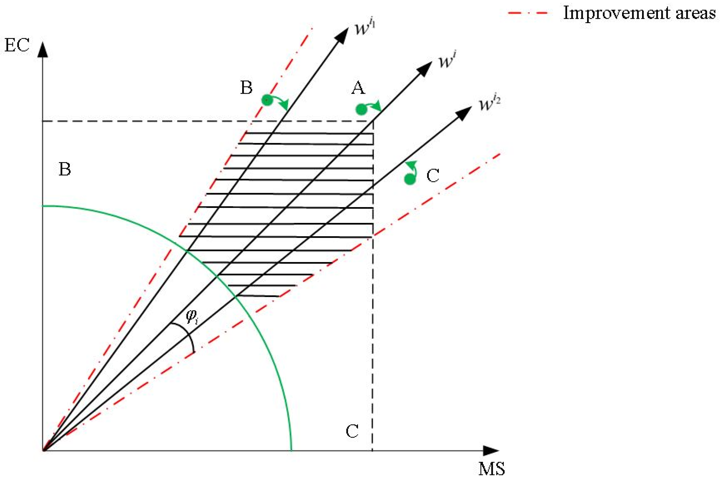
3.2. Strategy of Angle-Based Selection
3.3. Objective Normalization
4. Decomposition-Based Multi-Objective Artificial Bee Colony Algorithm
4.1. ABC Algorithm Basic Framework
| Algorithm 1. Fundamental structure of ABC algorithm |
| Run Procedure Initialize (); While Not Termination Condition() do Employed Bee searching for nectar (); Onlooker Bee to choose the honey source (); Scout Bee look for new nectar sources in their neighborhoods (); End While Deliver the finest solution (); End Procedure |
4.2. Initializing Populations
4.3. Encoding and Decoding
4.4. Changing Neighborhoods to Lead the Employed Bee Phase
- Segment insertion: randomly select segments from the segmented sequence vector and insert them into different randomly selected segments;
- Segment swap: randomly select two segments from the segmented sequence vector and swap their positions;
- Paint group mutation: randomly select segments from the paint group assignment matrix and change their assigned paint groups to different paint groups.
- Perform segmental painting insertion followed by painting panel mutation.
- Perform segmental swap followed by painting group mutation.
| Algorithm 2. Changing neighborhoods to lead the employed bee phase |
| For to do then ELse Endif then ; Endif then ; EndIf Endfor |
4.5. Collaborative Onlooker Bee Phase
| Algorithm 3. Collaborative onlooker bee phase |
| For to do ; ; ; then ; else ; Randomly select two distinct indexes r1,r2 that are different from I from E; Generate the offspring y by the Algorithm 2; Evaluate y and update ; Compute the angles between and y denoted as using(28); ; ; while () & (E is not null) do Randomly pick an index j from E; ; ; & then Replace with y, and set ; Remove j from E; end end |
4.6. Solving the Exchange of the Scout Bee Phase
| Algorithm 4. Solving the exchange of the employed bee phase |
| For to do then num is exchanged ← false; While is exchange=false then If Xi > then is exchange=true; Else ; End If then End End End |
4.7. The Complete Algorithmic Process
- N: the total of subproblems.
- wi (i = 1, …, N): uniformly distributed weight vectors.
- T: number of neighboring subproblems in a neighborhood.
- C: maximum number of consecutive failed updates for the current solution.
- L: number of consecutive failed iterations before discarding the solution.
- Step 1: Initialize the population, which contains N randomly generated solutions and N distributed weight vectors described in Section 4.2.
- Step 2: Update the population and the external population.
- Step 2.1: Perform the neighborhood-based switching method described in Section 4.4 applied to the employed bee phase.
- Step 2.2: Execute the angle selection strategy described in Section 4.5 applied to the collaborative onlooker bee phase.
- Step 2.3: Execute the solution-based switching described in Section 4.6 applied to the scout bee phase.
- Step 3: Repeat Step 2 until the termination condition is satisfied.
- Step 4: Update the external population and output.
5. Testing Study
5.1. Test Data
5.2. Performance Indicators
- Spread is a distributional metric that measures the Pareto frontier (PF), reflecting the degree of coverage of the solution set, with higher values indicating greater uniformity and better diversity, which is defined as follows:denotes the resulting PF, while representing the true solution set. represents the shortest Euclidean distance between the current solution i and the real solution set, and the average Euclidean distance is denoted by . and signify the total number of members and objectives, respectively. represents the Euclidean distance from objective j to the extreme solutions of the actual solution. Concerning this metric, smaller values are better.
- Generational distance (GD) represents the divergence between the acquired PF and the real PF, which measures the quality of convergence of the obtained PF, which is defined as follows:
- The Inverse Generation Distance (IGD) is a comprehensive metric, and it can be used to evaluate the distance and distribution between the solution set and the ideal solution, which is defined as follows:Here, stands for the minimum Euclidean distance between and the points within , with indicating the count of points in .
- The number of nondominated solutions (NOS) is used to indicate the number of nondominated solutions in the approximated true frontier, with larger values providing a better approximation of the entire true frontier.
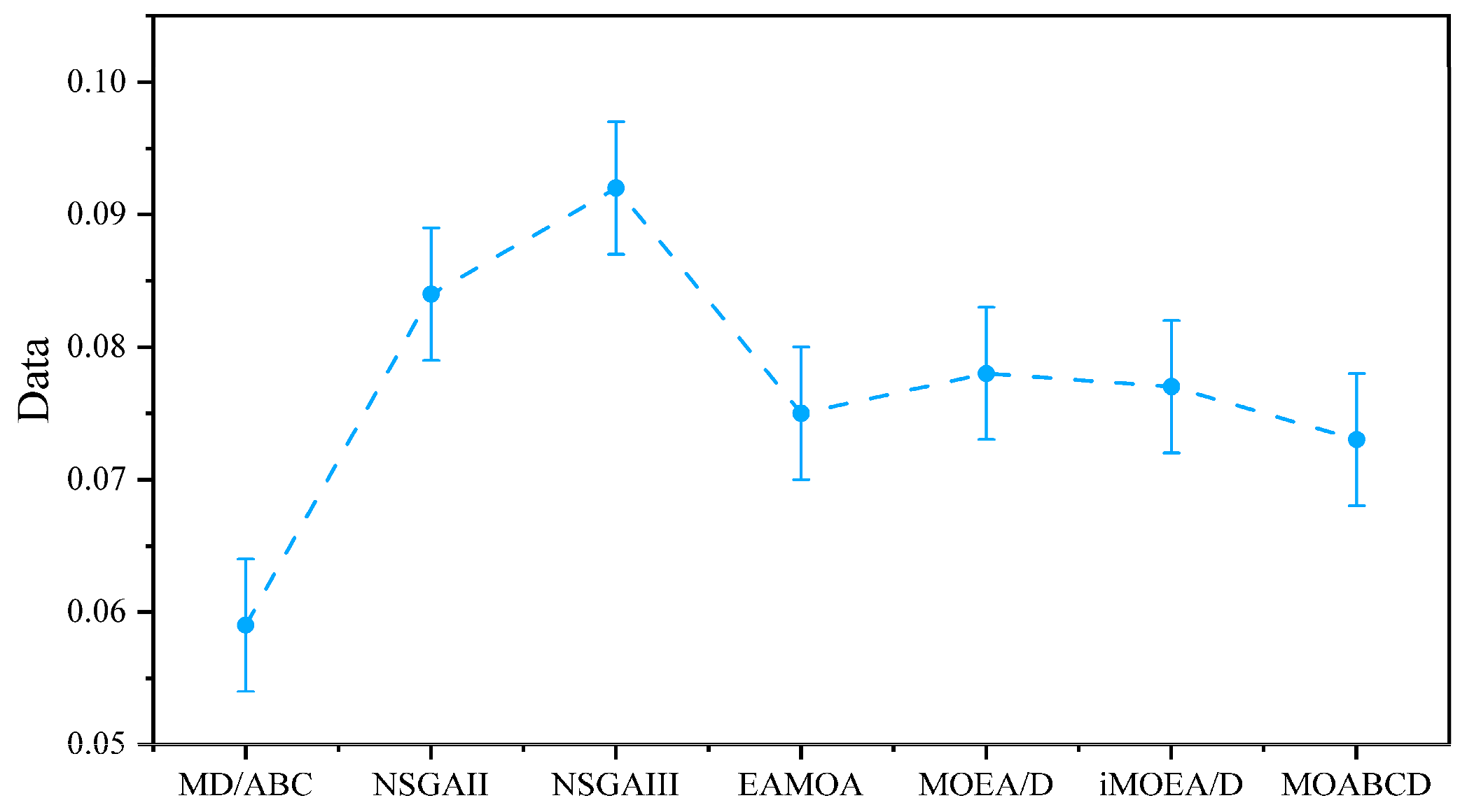
5.3. Parameter Settings
5.4. Evaluate the Core Strategy
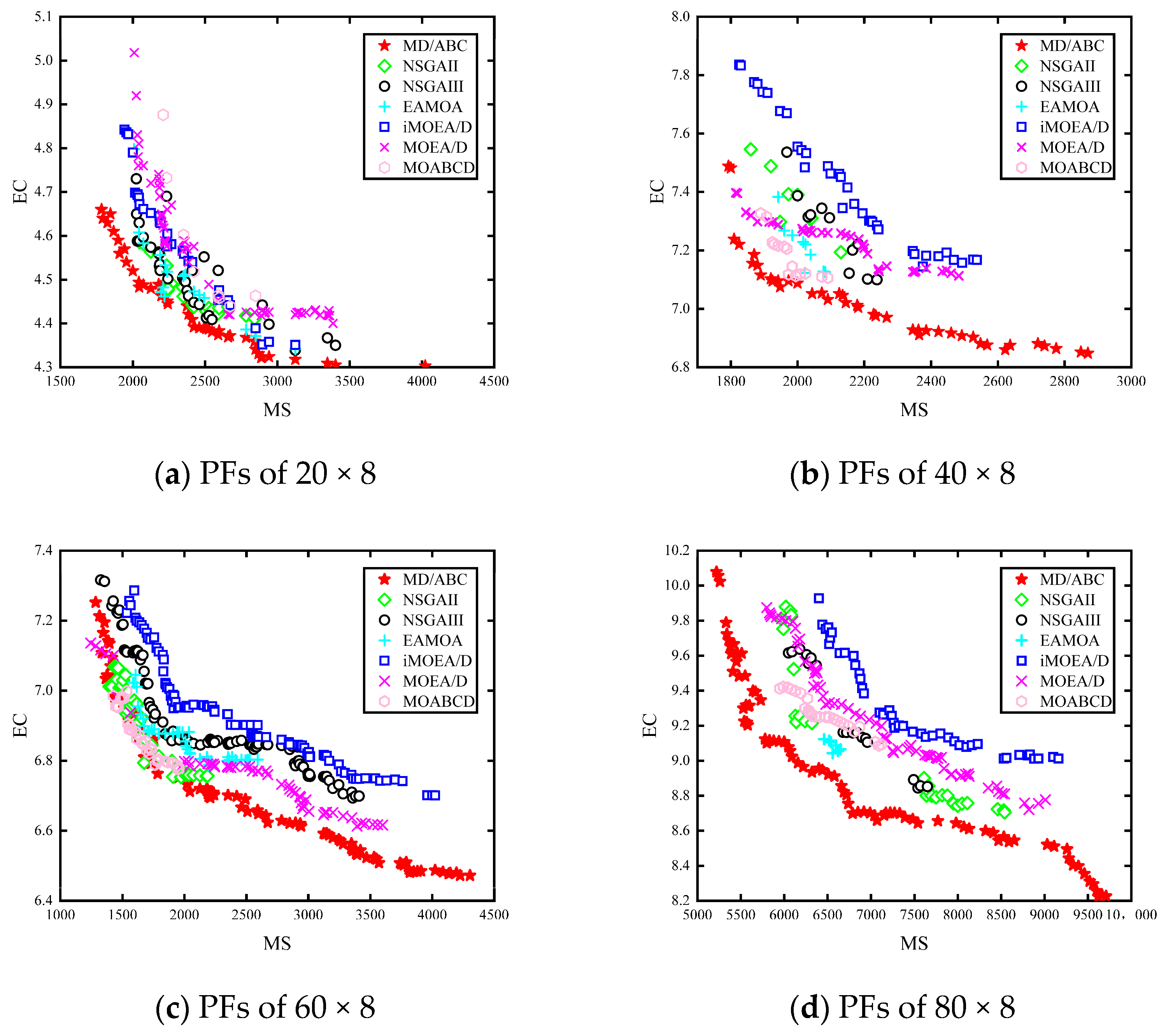
5.5. Evaluating the MD/ABC Algorithm
6. Conclusions and Future Work
Author Contributions
Funding
Institutional Review Board Statement
Informed Consent Statement
Data Availability Statement
Conflicts of Interest
References
- Yang, L.; Liu, Q.; Xia, T.; Ye, C.; Li, J. Preventive Maintenance Strategy Optimization in Manufacturing System Considering Energy Efficiency and Quality Cost. Energies 2022, 15, 8237. [Google Scholar] [CrossRef]
- Bu, H.; Yuan, X.; Niu, J.; Yu, W.; Ji, X.; Lyu, H.; Zhou, H. Ship Painting Process Design Based on IDBSACN-RF. Coatings 2021, 11, 1458. [Google Scholar] [CrossRef]
- Song, M.Y.; Chun, H. Species and Characteristics of Volatile Organic Compounds Emitted from an Auto-Repair Painting Workshop. Sci. Rep. 2021, 11, 16586. [Google Scholar] [CrossRef]
- Wang, Y.; Cao, Q.; Liu, L.; Wu, Y.; Liu, H.; Gu, Z.; Zhu, C. A Review of Low and Zero Carbon Fuel Technologies: Achieving Ship Carbon Reduction Targets. Sustain. Energy Technol. Assess. 2022, 54, 102762. [Google Scholar] [CrossRef]
- Kwon, B.; Lee, G.M. Spatial Scheduling for Large Assembly Blocks in Shipbuilding. Comput. Ind. Eng. 2015, 89, 203–212. [Google Scholar] [CrossRef]
- Cho, K.K.; Chung, K.H.; Park, C.; Park, J.C.; Kim, H.S. A Spatial Scheduling System for Block Painting Process in Shipbuilding. CIRP Ann. 2001, 50, 339–342. [Google Scholar] [CrossRef]
- Wang, Z.; Ma, Y.; Sun, Y.; Tang, H.; Cao, M.; Xia, R.; Han, F. Optimizing Energy Management and Case Study of Multi-Energy Coupled Supply for Green Ships. J. Mar. Sci. Eng. 2023, 11, 1286. [Google Scholar] [CrossRef]
- Qiao, Q.; Eskandari, H.; Saadatmand, H.; Sahraei, M.A. An Interpretable Multi-Stage Forecasting Framework for Energy Consumption and CO2 Emissions for the Transportation Sector. Energy 2024, 286, 129499. [Google Scholar] [CrossRef]
- Zhang, Y.; Sun, L.; Ma, F.; Wu, Y.; Jiang, W.; Fu, L. Collaborative Optimization of the Battery Capacity and Sailing Speed Considering Multiple Operation Factors for a Battery-Powered Ship. World Electr. Veh. J. 2022, 13, 40. [Google Scholar] [CrossRef]
- Xiang, Y.; Wu, G.; Shen, X.; Ma, Y.; Gou, J.; Xu, W.; Liu, J. Low-Carbon Economic Dispatch of Electricity-Gas Systems. Energy 2021, 226, 120267. [Google Scholar] [CrossRef]
- Wu, X.; Sun, Y. A Green Scheduling Algorithm for Flexible Job Shop with Energy-Saving Measures. J. Clean. Prod. 2018, 172, 3249–3264. [Google Scholar] [CrossRef]
- Geetha, M.; Chandra Guru Sekar, R.; Marichelvam, M.K.; Tosun, Ö. A Sequential Hybrid Optimization Algorithm (SHOA) to Solve the Hybrid Flow Shop Scheduling Problems to Minimize Carbon Footprint. Processes 2024, 12, 143. [Google Scholar] [CrossRef]
- Neufeld, J.S.; Schulz, S.; Buscher, U. A Systematic Review of Multi-Objective Hybrid Flow Shop Scheduling. Eur. J. Oper. Res. 2023, 309, 1–23. [Google Scholar] [CrossRef]
- Yu, C.; Andreotti, P.; Semeraro, Q. Multi-Objective Scheduling in Hybrid Flow Shop: Evolutionary Algorithms Using Multi-Decoding Framework. Comput. Ind. Eng. 2020, 147, 106570. [Google Scholar] [CrossRef]
- Qiu, Y.; Wang, J. A Machine Learning Approach to Credit Card Customer Segmentation for Economic Stability. In Proceedings of the 4th International Conference on Economic Management and Big Data Applications, ICEMBDA 2023, Tianjin, China, 27–29 October 2023; EAI: Tianjin, China, 2024. [Google Scholar]
- Heydarpoor, F.; Karbassi, S.M.; Bidabadi, N.; Ebadi, M.J. Solving Multi-Objective Functions for Cancer Treatment by Using Metaheuristic Algorithms. Int. J. Comb. Optim. Probl. Inform. 2020, 11, 61. [Google Scholar]
- Homaee, O.; Kazempour, A.; Gholami, A. Investigation of the Impacts of the Refill Valve Diameter on Prestrike Occurrence in Gas Circuit Breakers. Phys. Fluids 2021, 33, 087120. [Google Scholar] [CrossRef]
- Luan, F.; Cai, Z.; Wu, S.; Liu, S.Q.; He, Y. Optimizing the Low-Carbon Flexible Job Shop Scheduling Problem with Discrete Whale Optimization Algorithm. Mathematics 2019, 7, 688. [Google Scholar] [CrossRef]
- Wang, Z.; Shen, L.; Li, X.; Gao, L. An Improved Multi-Objective Firefly Algorithm for Energy-Efficient Hybrid Flowshop Rescheduling Problem. J. Clean. Prod. 2023, 385, 135738. [Google Scholar] [CrossRef]
- Wang, J.; Zheng, Y.; Huang, P.; Peng, H.; Wu, Z. A Stable-State Multi-Objective Evolutionary Algorithm Based on Decomposition. Expert Syst. Appl. 2024, 239, 122452. [Google Scholar] [CrossRef]
- Fan, M.; Chen, J.; Xie, Z.; Ouyang, H.; Li, S.; Gao, L. Improved Multi-Objective Differential Evolution Algorithm Based on a Decomposition Strategy for Multi-Objective Optimization Problems. Sci. Rep. 2022, 12, 21176. [Google Scholar] [CrossRef] [PubMed]
- Mallipeddi, R.; Das, K.N. A Twin-Archive Guided Decomposition Based Multi/Many-Objective Evolutionary Algorithm. Swarm Evol. Comput. 2022, 71, 101082. [Google Scholar]
- Xiang, Y.; Zhou, Y.; Tang, L.; Chen, Z. A Decomposition-Based Many-Objective Artificial Bee Colony Algorithm. IEEE Trans. Cybern. 2017, 49, 287–300. [Google Scholar] [CrossRef]
- Zhang, B.; Pan, Q.; Gao, L.; Meng, L.-L.; Li, X.-Y.; Peng, K.-K. A Three-Stage Multiobjective Approach Based on Decomposition for an Energy-Efficient Hybrid Flow Shop Scheduling Problem. IEEE Trans. Syst. Man Cybern. Syst. 2019, 50, 4984–4999. [Google Scholar] [CrossRef]
- Li, K.; Deb, K.; Zhang, Q.; Kwong, S. An Evolutionary Many-Objective Optimization Algorithm Based on Dominance and Decomposition. IEEE Trans. Evol. Comput. 2014, 19, 694–716. [Google Scholar] [CrossRef]
- Chen, J.; Ding, J.; Tan, K.C.; Chen, Q. A Decomposition-Based Evolutionary Algorithm for Scalable Multi/Many-Objective Optimization. Memetic Comp. 2021, 13, 413–432. [Google Scholar] [CrossRef]
- Zou, J.; Liu, J.; Yang, S.; Zheng, J. A Many-Objective Evolutionary Algorithm Based on Rotation and Decomposition. Swarm Evol. Comput. 2021, 60, 100775. [Google Scholar] [CrossRef]
- Chen, L.; Gan, W.; Li, H.; Cheng, K.; Pan, D.; Chen, L.; Zhang, Z. Solving Multi-Objective Optimization Problem Using Cuckoo Search Algorithm Based on Decomposition. Appl. Intell. 2021, 51, 143–160. [Google Scholar] [CrossRef]
- Zhou, J.; Zou, J.; Yang, S.; Zheng, J.; Gong, D.; Pei, T. Niche-Based and Angle-Based Selection Strategies for Many-Objective Evolutionary Optimization. Inf. Sci. 2021, 571, 133–153. [Google Scholar] [CrossRef]
- Shi, L.; Tan, Y.; Yan, Z.; Meng, L.; Liu, L. Weight Grouping Operators Selection Strategy for a Multiobjective Evolutionary Algorithm Based on Decomposition. Appl. Intell. 2023, 53, 10585–10601. [Google Scholar] [CrossRef]
- Katragjini, K.; Vallada, E.; Ruiz, R. Flow Shop Rescheduling under Different Types of Disruption. Int. J. Prod. Res. 2013, 51, 780–797. [Google Scholar] [CrossRef]
- Yilmaz Acar, Z.; Başçiftçi, F. Solving Multi-Objective Resource Allocation Problem Using Multi-Objective Binary Artificial Bee Colony Algorithm. Arab. J. Sci. Eng. 2021, 46, 8535–8547. [Google Scholar] [CrossRef]
- Zhang, W.; Li, Y. A Many-Objective Artificial Bee Colony Algorithm Based on Adaptive Grid. IEEE Access 2021, 9, 97138–97151. [Google Scholar] [CrossRef]
- Ramón-Canul, L.G.; Margarito-Carrizal, D.L.; Limón-Rivera, R.; Morales-Carrrera, U.A.; Rodríguez-Buenfil, I.M.; Ramírez-Sucre, M.O.; Cabal-Prieto, A.; Herrera-Corredor, J.A.; De Jesús Ramírez-Rivera, E. Technique for Order of Preference by Similarity to Ideal Solution (TOPSIS) Method for the Generation of External Preference Mapping Using Rapid Sensometric Techniques. J. Sci. Food. Agric. 2021, 101, 3298–3307. [Google Scholar] [CrossRef] [PubMed]
- Zhang, B.; Pan, Q.; Meng, L.; Zhang, X.; Jiang, X. A Decomposition-Based Multi-Objective Evolutionary Algorithm for Hybrid Flowshop Rescheduling Problem with Consistent Sublots. Int. J. Prod. Res. 2023, 61, 1013–1038. [Google Scholar] [CrossRef]
- Audet, C.; Bigeon, J.; Cartier, D.; Le Digabel, S.; Salomon, L. Performance Indicators in Multiobjective Optimization. Eur. J. Oper. Res. 2021, 292, 397–422. [Google Scholar] [CrossRef]
- Li, K.; Yan, X.; Han, Y.; Ge, F.; Jiang, Y. Many-Objective Optimization Based Path Planning of Multiple UAVs in Oilfield Inspection. Appl. Intell. 2022, 52, 12668–12683. [Google Scholar] [CrossRef]
- Ozcelikkan, N.; Tuzkaya, G.; Alabas-Uslu, C.; Sennaroglu, B. A Multi-Objective Agile Project Planning Model and a Comparative Meta-Heuristic Approach. Inf. Softw. Technol. 2022, 151, 107023. [Google Scholar] [CrossRef]
- Kuncoro, I.W.; Pambudi, N.A.; Biddinika, M.K.; Budiyanto, C.W. Optimization of Immersion Cooling Performance Using the Taguchi Method. Case Stud. Therm. Eng. 2020, 21, 100729. [Google Scholar] [CrossRef]
- Deb, K.; Pratap, A.; Agarwal, S.; Meyarivan, T. A Fast and Elitist Multiobjective Genetic Algorithm: NSGA-II. IEEE Trans. Evol. Comput. 2002, 6, 182–197. [Google Scholar] [CrossRef]
- Jain, H.; Deb, K. An Evolutionary Many-Objective Optimization Algorithm Using Reference-Point Based Nondominated Sorting Approach, Part II: Handling Constraints and Extending to an Adaptive Approach. IEEE Trans. Evol. Comput. 2013, 18, 602–622. [Google Scholar] [CrossRef]
- Ho-Huu, V.; Hartjes, S.; Visser, H.G.; Curran, R. An Improved MOEA/D Algorithm for Bi-Objective Optimization Problems with Complex Pareto Fronts and Its Application to Structural Optimization. Expert Syst. Appl. 2018, 92, 430–446. [Google Scholar] [CrossRef]
- Li, J.; Sang, H.; Han, Y.; Wang, C.; Gao, K. Efficient Multi-Objective Optimization Algorithm for Hybrid Flow Shop Scheduling Problems with Setup Energy Consumptions. J. Clean. Prod. 2018, 181, 584–598. [Google Scholar] [CrossRef]
- Li, X.; Ma, S. Multiobjective Discrete Artificial Bee Colony Algorithm for Multiobjective Permutation Flow Shop Scheduling Problem with Sequence Dependent Setup Times. IEEE Trans. Eng. Manag. 2017, 64, 149–165. [Google Scholar] [CrossRef]


| Symbol | Meaning |
|---|---|
| Set of painting teams at the stage and | |
| A grouping of positions designed to accommodate segments allocated to individual painting teams and | |
| Segment j Processing time for the segmental painting team on the stage | |
| Setup time from segment to stage represents that segment is the first segment assigned to a painting team | |
| Transportation from painting team m on stage | |
| Setup energy consumption from segment in stage . indicates that segment j is the first segmental painting team assigned at stage | |
| Energy consumption of the painting team in process on stage | |
| Energy consumption of the painting team at idle on stage | |
| Energy consumption of transportation equipment between in a given phase | |
| Equipment energy utilization for the painting team on stage | |
| Start time for the segment during the stage | |
| Ending time for the segment during the stage | |
| The outset time for the segment at the position within painting team | |
| The finish time for the segment at the position within painting team | |
| The binary variable equals when segment is allocated to position of painting team m during stage , and 0 otherwise | |
| The binary variable equals if segment necessitates transportation at stage ; otherwise, it equals | |
| The intermediate variable denotes the energy consumption of the painting team on stage when it stays in the adjusted and idle state from position to position , and denotes the initial adjusted energy consumption of the first segmental painting team assigned to it | |
| The intermediate variable indicates the energy consumption to transport segment from a particular stage to stage |
| Factors | Levels | Number of Levels |
|---|---|---|
| Number of segments | 20, 40, 60, 80, 100 | 5 |
| Number of stages | 3, 5, 8, 10 | 4 |
| Number of painting teams per stage | [1,5] | 1 |
| Transportation time | [1,25] | 1 |
| Basic processing time | [1,99] | 1 |
| Conversion factor | 1 | |
| Adjustment time | U[1,25], U[1,49], U[1,99], U[1,124] | 4 |
| Adjustment energy consumption | [2,5] | 1 |
| Idle energy consumption | [1,3] | 1 |
| Parameter | Parameter Level | |||
|---|---|---|---|---|
| 1 | 2 | 3 | 4 | |
| N | 100 | 150 | 200 | 250 |
| M | 2 | 3 | 5 | 8 |
| T | 5 | 10 | 15 | 20 |
| C | 8 | 10 | 15 | 18 |
| L | 20 | 30 | 50 | 80 |
| Experiment Number | Parameter | AVG | ||||
|---|---|---|---|---|---|---|
| N | M | T | C | L | ||
| 1 | 100 | 2 | 5 | 8 | 20 | 0.0904 |
| 2 | 100 | 3 | 10 | 10 | 30 | 0.0922 |
| 3 | 100 | 5 | 15 | 15 | 50 | 0.0873 |
| 4 | 100 | 8 | 20 | 18 | 80 | 0.0762 |
| 5 | 150 | 2 | 10 | 15 | 80 | 0.0785 |
| 6 | 150 | 3 | 5 | 18 | 50 | 0.0931 |
| 7 | 150 | 5 | 20 | 8 | 30 | 0.0792 |
| 8 | 150 | 8 | 15 | 10 | 20 | 0.0901 |
| 9 | 200 | 2 | 15 | 18 | 30 | 0.0882 |
| 10 | 200 | 3 | 20 | 15 | 20 | 0.0742 |
| 11 | 200 | 5 | 5 | 10 | 80 | 0.0942 |
| 12 | 200 | 8 | 10 | 8 | 50 | 0.0933 |
| 13 | 250 | 2 | 20 | 10 | 50 | 0.0543 |
| 14 | 250 | 3 | 15 | 8 | 80 | 0.0921 |
| 15 | 250 | 5 | 10 | 18 | 20 | 0.1255 |
| 16 | 250 | 8 | 5 | 15 | 30 | 0.1121 |
| Level | N | M | T | C | L |
|---|---|---|---|---|---|
| 1 | 0.0865 | 0.0779 | 0.0975 | 0.0886 | 0.0951 |
| 2 | 0.0852 | 0.0879 | 0.0974 | 0.0827 | 0.0929 |
| 3 | 0.0875 | 0.0966 | 0.0894 | 0.0880 | 0.0820 |
| 4 | 0.0960 | 0.0929 | 0.0710 | 0.0958 | 0.0853 |
| Rank | 4 | 3 | 2 | 5 | 1 |
| Problem | MD/ABC | MD/ABCa | MD/ABCs |
|---|---|---|---|
| 20 × 3 | 0.074 | 0.072 | 0.124 |
| 20 × 5 | 0.086 | 0.081 | 0.153 |
| 20 × 8 | 0.095 | 0.145 | 0.192 |
| 20 × 10 | 0.142 | 0.136 | 0.188 |
| 40 × 3 | 0.082 | 0.076 | 0.143 |
| 40 × 5 | 0.144 | 0.212 | 0.234 |
| 40 × 8 | 0.096 | 0.098 | 0.165 |
| 40 × 10 | 0.181 | 0.178 | 0.242 |
| 60 × 3 | 0.165 | 0.162 | 0.231 |
| 60 × 5 | 0.114 | 0.132 | 0.199 |
| 60 × 8 | 0.144 | 0.139 | 0.233 |
| 60 × 10 | 0.111 | 0.163 | 0.187 |
| 80 × 3 | 0.101 | 0.104 | 0.206 |
| 80 × 5 | 0.103 | 0.101 | 0.190 |
| 80 × 8 | 0.122 | 0.221 | 0.304 |
| 80 × 10 | 0.163 | 0.236 | 0.258 |
| 100 × 3 | 0.082 | 0.078 | 0.178 |
| 100 × 5 | 0.186 | 0.146 | 0.286 |
| 100 × 8 | 0.083 | 0.086 | 0.158 |
| 100 × 10 | 0.121 | 0.118 | 0.257 |
| Mean | 0.120 | 0.134 | 0.206 |
| Problem | MD/ABC | NSGAII | NSGAIII | EAMOA | MOEA/D | iMOEA/D | MOABCD |
|---|---|---|---|---|---|---|---|
| 20 × 3 | 0.725 | 1.178 | 1.362 | 0.954 | 0.864 | 0.754 | 0.815 |
| 20 × 5 | 0.517 | 1.122 | 1.143 | 0.966 | 0.673 | 0.709 | 0.743 |
| 20 × 8 | 0.613 | 1.083 | 1.113 | 0.975 | 0.726 | 0.694 | 0.740 |
| 20 × 10 | 0.611 | 1.058 | 1.024 | 0.954 | 0.984 | 0.752 | 0.819 |
| 40 × 3 | 0.629 | 1.162 | 1.216 | 0.932 | 0.762 | 0.769 | 0.796 |
| 40 × 5 | 0.617 | 1.167 | 1.243 | 0.965 | 0.843 | 0.748 | 0.738 |
| 40 × 8 | 0.612 | 1.147 | 1.257 | 0.944 | 0.720 | 0.753 | 0.836 |
| 40 × 10 | 0.681 | 1.095 | 1.087 | 0.939 | 0.735 | 0.691 | 0.726 |
| 60 × 3 | 0.621 | 1.106 | 1.098 | 0.812 | 0.697 | 0.736 | 0.744 |
| 60 × 5 | 0.701 | 1.136 | 1.145 | 0.923 | 0.802 | 0.707 | 0.812 |
| 60 × 8 | 0.642 | 1.105 | 1.101 | 0.824 | 0.817 | 0.662 | 0.772 |
| 60 × 10 | 0.741 | 1.082 | 1.017 | 0.912 | 0.846 | 0.795 | 0.783 |
| 80 × 3 | 0.015 | 1.225 | 1.125 | 0.924 | 0.811 | 0.654 | 0.785 |
| 80 × 5 | 0.547 | 1.071 | 1.165 | 0.905 | 0.898 | 0.745 | 0.753 |
| 80 × 8 | 0.124 | 1.067 | 1.154 | 0.956 | 0.983 | 0.681 | 0.703 |
| 80 × 10 | 0.499 | 1.074 | 1.098 | 0.912 | 0.978 | 0.758 | 0.762 |
| 100 × 3 | 0.712 | 1.212 | 1.232 | 0.976 | 0.801 | 0.736 | 0.728 |
| 100 × 5 | 0.649 | 1.078 | 1.178 | 0.934 | 0.905 | 0.690 | 0.764 |
| 100 × 8 | 0.641 | 1.129 | 1.178 | 0.859 | 0.816 | 0.656 | 0.879 |
| 100 × 10 | 0.578 | 1.102 | 1.095 | 0.992 | 0.992 | 0.723 | 0.898 |
| Mean | 0.574 | 1.120 | 1.152 | 0.928 | 0.833 | 0.721 | 0.780 |
| Problem | MD/ABC | NSGAII | NSGAIII | EAMOA | MOEA/D | iMOEA/D | MOABCD |
|---|---|---|---|---|---|---|---|
| 20 × 3 | 0.014 | 0.028 | 0.039 | 0.017 | 0.044 | 0.022 | 0.021 |
| 20 × 5 | 0.022 | 0.042 | 0.052 | 0.034 | 0.053 | 0.041 | 0.037 |
| 20 × 8 | 0.026 | 0.035 | 0.048 | 0.031 | 0.051 | 0.038 | 0.034 |
| 20 × 10 | 0.012 | 0.037 | 0.034 | 0.030 | 0.050 | 0.033 | 0.026 |
| 40 × 3 | 0.016 | 0.049 | 0.036 | 0.027 | 0.036 | 0.018 | 0.041 |
| 40 × 5 | 0.027 | 0.034 | 0.040 | 0.033 | 0.039 | 0.042 | 0.038 |
| 40 × 8 | 0.023 | 0.036 | 0.057 | 0.035 | 0.037 | 0.038 | 0.032 |
| 40 × 10 | 0.029 | 0.044 | 0.031 | 0.046 | 0.044 | 0.026 | 0.038 |
| 60 × 3 | 0.027 | 0.054 | 0.048 | 0.039 | 0.041 | 0.031 | 0.045 |
| 60 × 5 | 0.024 | 0.048 | 0.042 | 0.037 | 0.049 | 0.029 | 0.039 |
| 60 × 8 | 0.026 | 0.031 | 0.037 | 0.034 | 0.042 | 0.032 | 0.029 |
| 60 × 10 | 0.020 | 0.045 | 0.032 | 0.044 | 0.051 | 0.035 | 0.026 |
| 80 × 3 | 0.016 | 0.039 | 0.046 | 0.031 | 0.037 | 0.019 | 0.031 |
| 80 × 5 | 0.019 | 0.041 | 0.048 | 0.038 | 0.031 | 0.028 | 0.035 |
| 80 × 8 | 0.022 | 0.058 | 0.051 | 0.037 | 0.035 | 0.025 | 0.040 |
| 80 × 10 | 0.025 | 0.036 | 0.046 | 0.031 | 0.042 | 0.028 | 0.046 |
| 100 × 3 | 0.022 | 0.042 | 0.031 | 0.041 | 0.038 | 0.026 | 0.044 |
| 100 × 5 | 0.018 | 0.041 | 0.055 | 0.031 | 0.044 | 0.056 | 0.033 |
| 100 × 8 | 0.027 | 0.036 | 0.047 | 0.039 | 0.042 | 0.034 | 0.032 |
| 100 × 10 | 0.015 | 0.039 | 0.038 | 0.030 | 0.034 | 0.058 | 0.035 |
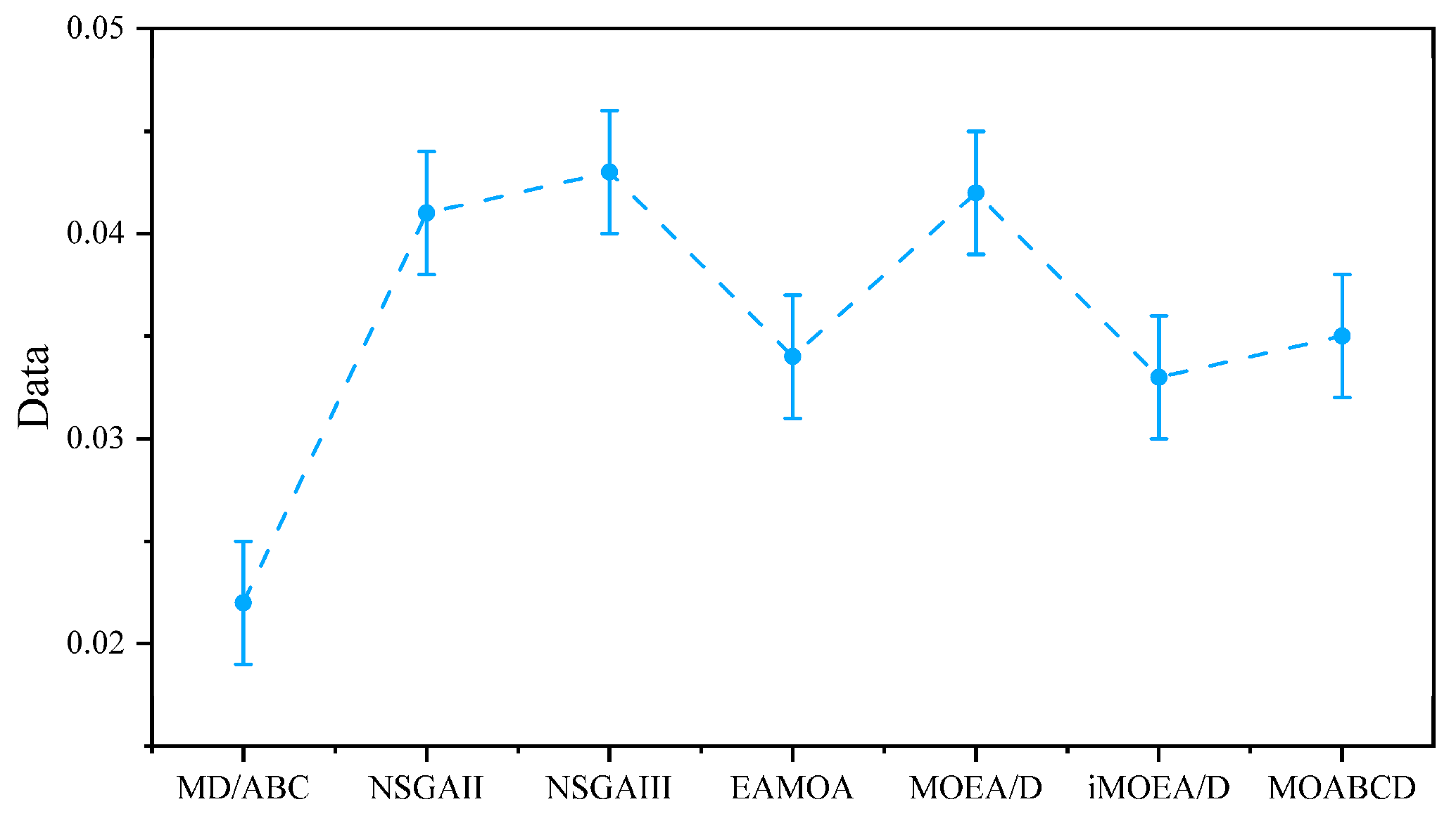
| Mean | 0.022 | 0.041 | 0.043 | 0.034 | 0.042 | 0.033 | 0.035 |
| Problem | MD/ABC | NSGAII | NSGAIII | EAMOA | MOEA/D | iMOEA/D | MOABCD |
|---|---|---|---|---|---|---|---|
| 20 × 3 | 0.064 | 0.088 | 0.097 | 0.074 | 0.076 | 0.074 | 0.079 |
| 20 × 5 | 0.045 | 0.117 | 0.108 | 0.068 | 0.071 | 0.082 | 0.082 |
| 20 × 8 | 0.047 | 0.096 | 0.102 | 0.080 | 0.074 | 0.081 | 0.054 |
| 20 × 10 | 0.053 | 0.081 | 0.124 | 0.063 | 0.069 | 0.076 | 0.067 |
| 40 × 3 | 0.037 | 0.072 | 0.094 | 0.074 | 0.075 | 0.079 | 0.052 |
| 40 × 5 | 0.063 | 0.076 | 0.106 | 0.072 | 0.068 | 0.073 | 0.068 |
| 40 × 8 | 0.067 | 0.080 | 0.086 | 0.076 | 0.079 | 0.078 | 0.075 |
| 40 × 10 | 0.072 | 0.085 | 0.079 | 0.082 | 0.087 | 0.080 | 0.071 |
| 60 × 3 | 0.062 | 0.087 | 0.079 | 0.071 | 0.083 | 0.083 | 0.077 |
| 60 × 5 | 0.048 | 0.063 | 0.082 | 0.075 | 0.084 | 0.078 | 0.061 |
| 60 × 8 | 0.058 | 0.078 | 0.081 | 0.079 | 0.088 | 0.061 | 0.065 |
| 60 × 10 | 0.063 | 0.087 | 0.086 | 0.068 | 0.085 | 0.076 | 0.070 |
| 80 × 3 | 0.057 | 0.083 | 0.103 | 0.072 | 0.076 | 0.077 | 0.074 |
| 80 × 5 | 0.072 | 0.088 | 0.087 | 0.077 | 0.086 | 0.071 | 0.088 |
| 80 × 8 | 0.054 | 0.082 | 0.099 | 0.081 | 0.078 | 0.075 | 0.076 |
| 80 × 10 | 0.071 | 0.086 | 0.086 | 0.084 | 0.086 | 0.074 | 0.082 |
| 100 × 3 | 0.061 | 0.074 | 0.089 | 0.074 | 0.072 | 0.076 | 0.085 |
| 100 × 5 | 0.072 | 0.077 | 0.076 | 0.073 | 0.074 | 0.084 | 0.074 |
| 100 × 8 | 0.062 | 0.089 | 0.091 | 0.083 | 0.080 | 0.075 | 0.086 |
| 100 × 10 | 0.061 | 0.083 | 0.093 | 0.082 | 0.077 | 0.085 | 0.081 |
| Mean | 0.059 | 0.084 | 0.092 | 0.075 | 0.078 | 0.077 | 0.073 |
| Problem | MD/ABC | NSGAII | NSGAIII | EAMOA | MOEA/D | iMOEA/D | MOABCD |
|---|---|---|---|---|---|---|---|
| 20 × 3 | 63 | 55 | 47 | 42 | 42 | 46 | 6 |
| 20 × 5 | 79 | 34 | 22 | 47 | 27 | 31 | 11 |
| 20 × 8 | 43 | 21 | 36 | 16 | 33 | 27 | 8 |
| 20 × 10 | 52 | 26 | 38 | 8 | 50 | 36 | 17 |
| 40 × 3 | 92 | 16 | 21 | 23 | 81 | 82 | 32 |
| 40 × 5 | 51 | 12 | 8 | 16 | 37 | 31 | 16 |
| 40 × 8 | 42 | 9 | 11 | 9 | 34 | 40 | 14 |
| 40 × 10 | 49 | 6 | 19 | 7 | 34 | 36 | 23 |
| 60 × 3 | 87 | 39 | 32 | 25 | 72 | 74 | 26 |
| 60 × 5 | 71 | 17 | 24 | 8 | 69 | 59 | 10 |
| 60 × 8 | 54 | 13 | 31 | 18 | 37 | 41 | 11 |
| 60 × 10 | 52 | 12 | 15 | 7 | 42 | 40 | 14 |
| 80 × 3 | 106 | 83 | 46 | 38 | 84 | 73 | 12 |
| 80 × 5 | 84 | 27 | 37 | 10 | 70 | 69 | 27 |
| 80 × 8 | 39 | 22 | 22 | 16 | 32 | 24 | 30 |
| 80 × 10 | 67 | 13 | 14 | 19 | 65 | 54 | 16 |
| 100 × 3 | 77 | 61 | 49 | 44 | 74 | 53 | 31 |
| 100 × 5 | 47 | 36 | 25 | 25 | 29 | 32 | 15 |
| 100 × 8 | 65 | 11 | 13 | 13 | 54 | 55 | 14 |
| 100 × 10 | 52 | 23 | 17 | 8 | 36 | 31 | 17 |
| Mean | 64 | 27 | 26 | 20 | 50 | 47 | 18 |
Disclaimer/Publisher’s Note: The statements, opinions and data contained in all publications are solely those of the individual author(s) and contributor(s) and not of MDPI and/or the editor(s). MDPI and/or the editor(s) disclaim responsibility for any injury to people or property resulting from any ideas, methods, instructions or products referred to in the content. |
© 2024 by the authors. Licensee MDPI, Basel, Switzerland. This article is an open access article distributed under the terms and conditions of the Creative Commons Attribution (CC BY) license (https://creativecommons.org/licenses/by/4.0/).
Share and Cite
Bu, H.; Zhu, X.; Ge, Z.; Yang, T.; Yan, Z.; Tang, Y. A Decomposition-Based Multi-Objective Evolutionary Algorithm for Solving Low-Carbon Scheduling of Ship Segment Painting. Coatings 2024, 14, 368. https://0-doi-org.brum.beds.ac.uk/10.3390/coatings14030368
Bu H, Zhu X, Ge Z, Yang T, Yan Z, Tang Y. A Decomposition-Based Multi-Objective Evolutionary Algorithm for Solving Low-Carbon Scheduling of Ship Segment Painting. Coatings. 2024; 14(3):368. https://0-doi-org.brum.beds.ac.uk/10.3390/coatings14030368
Chicago/Turabian StyleBu, Henan, Xianpeng Zhu, Zikang Ge, Teng Yang, Zhuwen Yan, and Yingxin Tang. 2024. "A Decomposition-Based Multi-Objective Evolutionary Algorithm for Solving Low-Carbon Scheduling of Ship Segment Painting" Coatings 14, no. 3: 368. https://0-doi-org.brum.beds.ac.uk/10.3390/coatings14030368