A Physically Consistent Model for Forced Torsional Vibrations of Automotive Driveshafts

Abstract

The aim of this research was to design a physically consistent model for the forced torsional vibrations of automotive driveshafts that considered aspects of the following phenomena: excitation due to the transmission of the combustion engine through the gearbox, excitation due to the road geometry, the quasi-isometry of the automotive driveshaft, the effect of nonuniformity of the inertial moment with respect to the longitudinal axis of the tulip–tripod joint and of the bowl–balls–inner race joint, the torsional rigidity, and the torsional damping of each joint. To resolve the equations of motion describing the forced torsional nonlinear parametric vibrations of automotive driveshafts, a variational approach that involves Hamilton’s principle was used, which considers the isometric nonuniformity, where it is known that the joints of automotive driveshafts are quasi-isometric in terms of the twist angle, even if, in general, they are considered CVJs (constant velocity joints). This effect realizes the link between the terms for the torsional vibrations between the elements of the driveshaft: tripode–tulip, midshaft, and bowl–balls–inner race joint elements. The induced torsional loads (as gearbox torsional moments that enter the driveshaft through the tulip axis) can be of harmonic type, while the reactive torsional loads (as reactive torsional moments that enter the driveshaft through the bowl axis) are impulsive. These effects induce the resulting nonlinear dynamic behavior. Also considered was the effect of nonuniformity on the axial moment of inertia of the tripod–tulip element as well as on the axial moment of inertia of the bowl–balls–inner race joint element, that vary with the twist angle of each element. This effect induces parametric dynamic behavior. Moreover, the torsional rigidity was taken into consideration, as was the torsional damping for each joint of the driveshaft: tripod–joint and bowl–balls–inner race joint. This approach was used to obtain a system of equations of nonlinear partial derivatives that describes the torsional vibrations of the driveshaft as nonlinear parametric dynamic behavior. This model was used to compute variation in the natural frequencies of torsion in the global tulip (a given imposed geometry) using the angle between the tulip–midshaft for an automotive driveshaft designed for heavy-duty SUVs as well as the characteristic amplitude frequency in the region of principal parametric resonance together the method of harmonic balance for the steady-state forced torsional nonlinear vibration of the driveshaft. This model of dynamic behavior for the driveshaft can be used during the early stages of design as well in predicting the durability of automotive driveshafts. In addition, it is important that this model be added in the design algorithm for predicting the comfort elements of the automotive environment to adequately account for this kind of dynamic behavior that induces excitations in the car structure.

1. Introduction

The present work presents a consistent model to describe the forced torsional vibrations of an automotive driveshaft considering the following aspects: the joints of the driveshaft are quasi-isometric in terms of angular velocity [1] even if they are generally considered to be CVJs (constant velocity joints); the effect of induced torsional loads such as the harmonic entry moment from the gearbox [2] (p. 360) and the impulsive reaction moment from the wheels [3]; the effect of nonuniformity on the axial moment of inertia of the joints that varies with the angle of twist of each element of the driveshaft, and the effect of the torsional rigidity as well as the torsional damping for each joint of the driveshaft, which varies with the angle of twist of each element of the driveshaft. In the literature [4], the nonuniformity in the isometric properties of automotive driveshafts is already a fact recognized for more than half a century whose reality was demonstrated in experiments performed by Steinwede for his Ph.D. thesis [5] (pp. 68–97). This nonuniformity in driveshaft isometric properties is undoubtedly the main cause of nonlinear parametric vibrations of driveshafts in the range 0.1–12 kHz as established by experimental results documented in the literature [5] (pp. 98–123). The first researchers who considered the special dynamic phenomena of driveshafts were Mazzei and Scott, who enhanced the nonlinear parametric dynamic behavior of a universal joint in their paper [6]. The experimental evidence for nonuniformity of CVJ driveshaft transmission is presented and highlighted by Browne and Palazzolo in [7]. Moreover, in Feng, Rakheja, and Shangguan [8], optimization of the generated axial force (GAF) of a driveshaft system with the interval of uncertainty was treated without considering the CVJ isometry of the driveshaft, which is no longer isometric, and this aspect has been certified by experiments using the vertex method for analysis of the upper and lower bond (ULB) variation in parameters. In [9], Tiberiu-Petrescu mentioned the angular velocity variation for a double-cardan transmission, while paper [10] deals with the use of six sigma methodology for optimization of the cardan shaft transmission of light truck driveshafts because, in the exploitation, it is necessary to mitigate the vibration noise harshness. In [10], the authors mention the presence of vibration noise harshness due to the driveshaft but did not research why these phenomena were present. In a master’s degree thesis [11], the author developed a software based on MATLAB’s Simulink to realize the modeling and simulation of vehicle kinematics and dynamics, but the models of vehicle transmission were very simple and did not touch upon special phenomena of vehicle transmission. The design and stress analysis for an automobile driveshaft made of composite material is presented in [12], whereby the transmission is designed in such a way that the researchers’ special phenomena that are not well explained are avoided. In the literature, it is highlighted that an active steering control strategy can be used to prevent vehicle rollover [13], or a hierarchical synchronization control strategy can be used for the ARIS system to overcome the synchronization errors induced by the wheels [14]. As can be seen, none of these examples addresses the nonuniformity from the geometric and kinematic isometry of the automotive driveshaft. In the literature [15], some studies were conducted on optimizing the high-frequency torsional vibration of vehicle driveline systems using genetic algorithms, meaning that the designers and fabricants already found strange dynamic phenomena and tried to overcome these problems. Other researchers tried to diagnose defects of the drive system based on the vibration signal reference model [16]. Alugongo, in [17], continued the investigation of Mazzei and Scott [6] and Browne and Palazzolo [7] but only for a cardan shaft, which has already been demonstrated, by theory and experiments, to induce parametric vibrations. Xu, Zhu, and Xia analyzed the amplitude-frequency characteristics of torsional vibration for an entire automotive powertrain [18] using a model with 29 degrees of freedom. An approach for the nonlinear torsional vibrations of the automotive drivetrain using a model with three degrees of freedom is presented in [19], where the torsional stiffness and friction moment of a clutch system were measured and used to calibrate the model. This model in [19] is not a nonlinear parametric model of torsional vibration that depends on the mass moments of inertia; the geometrical moments of inertia; the geometrical positions of the tulip mass center, tulip axis mass center, bowl mass center, and bowl axis mass center; and nonuniformity in the geometric axial moments of inertia, mass axial moments of inertia for the driveshaft elements, and geometric and kinematic isometry of the driveshaft. As can be seen from the literature survey, the information concerning the details of CVJ driveshaft investigation of nonlinear parametric dynamic behavior, especially the MDPI journals, is unfortunately very poor in presenting such subjects, not because it is less important for the design area and automotive industry but because it involves a huge investment in experimental research, most of which involves intellectual property, through patents, of the biggest corporations in the car industry such as Renault, Daimler-Benz, BMW, GMC, Chrysler, Audi-VW Group, etc.

The goal of this study was to establish a complete dynamic model for an automotive CVJ quasi-homokinetic driveshaft model that includes elements describing the nonlinear forced parametric dynamic behavior. It is envisaged that this model can be used in the early stages of design as well as in predicting the durability of automotive driveshafts.

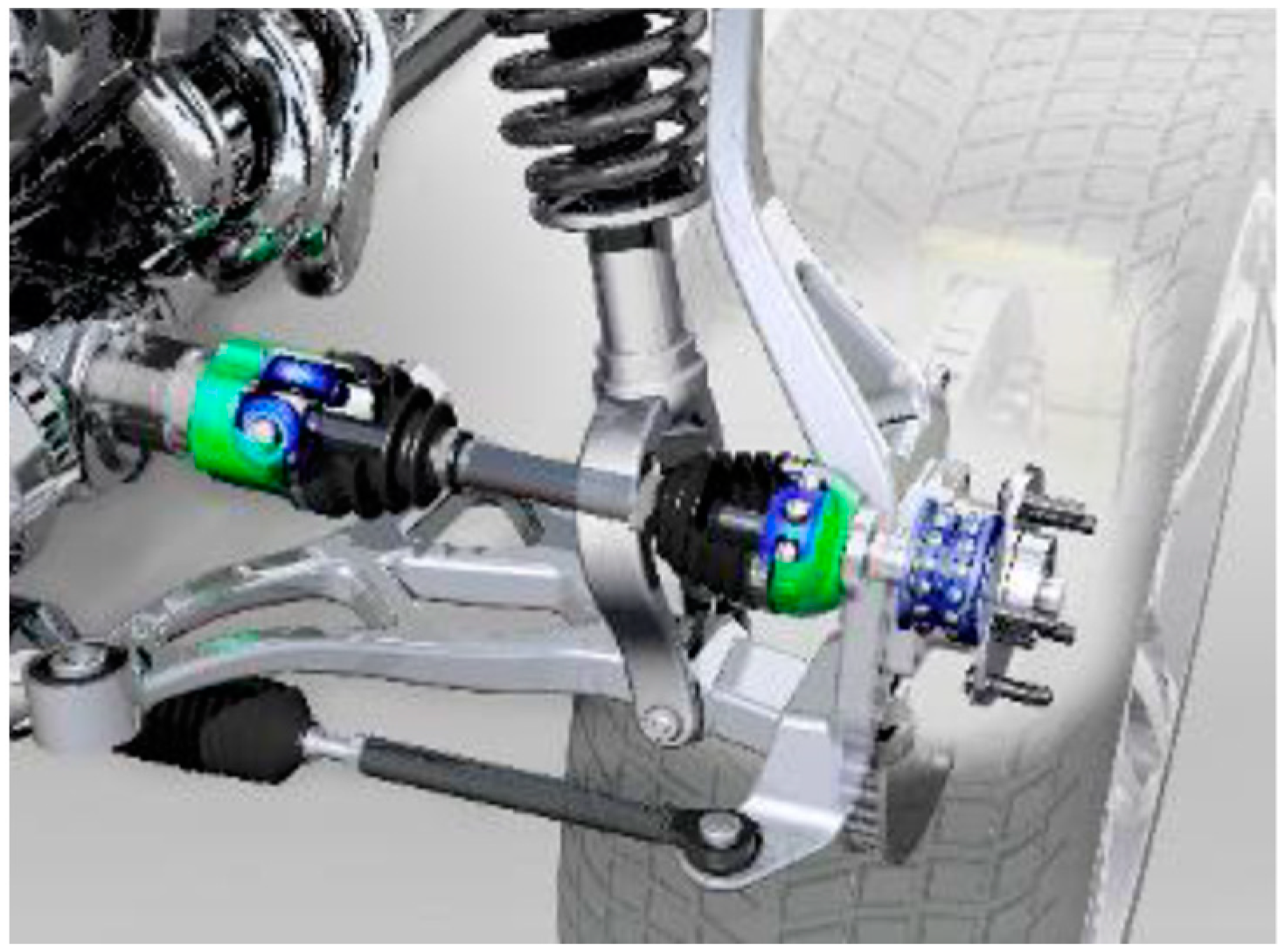
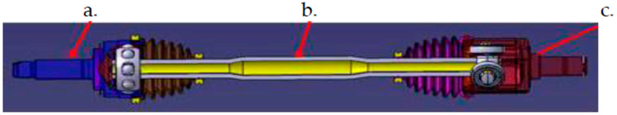
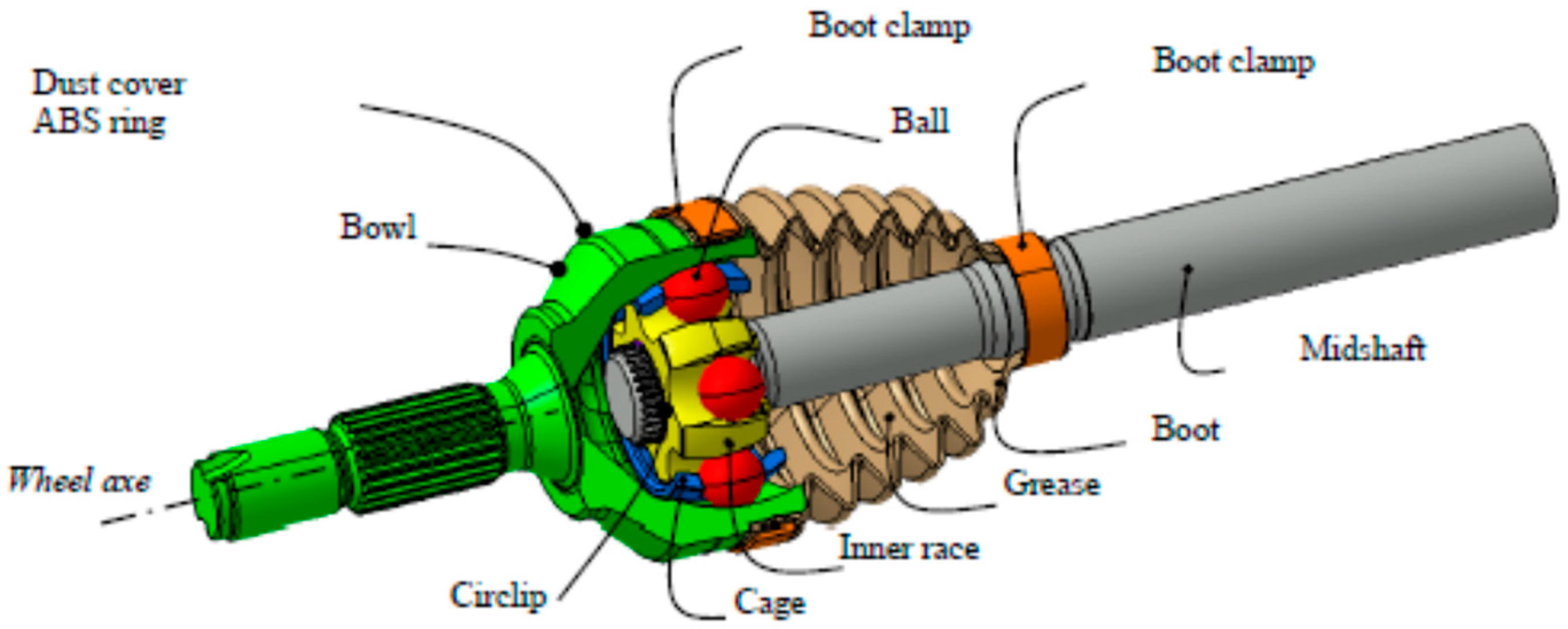
A driveshaft is a mechanism that transmits a torque load from the gearbox to the wheel, as can be seen in Figure 1. For a better geometrical understanding, let us look inside the components of such a mechanism, shown in Figure 2, that consists of (a) the bowl-balls joint fixed assembled with the car wheel, (b) the midshaft axis, (c) the tulip-tripode joint that allows axial plunging of the tripode in the tulip and plunging assembled in the gear box.

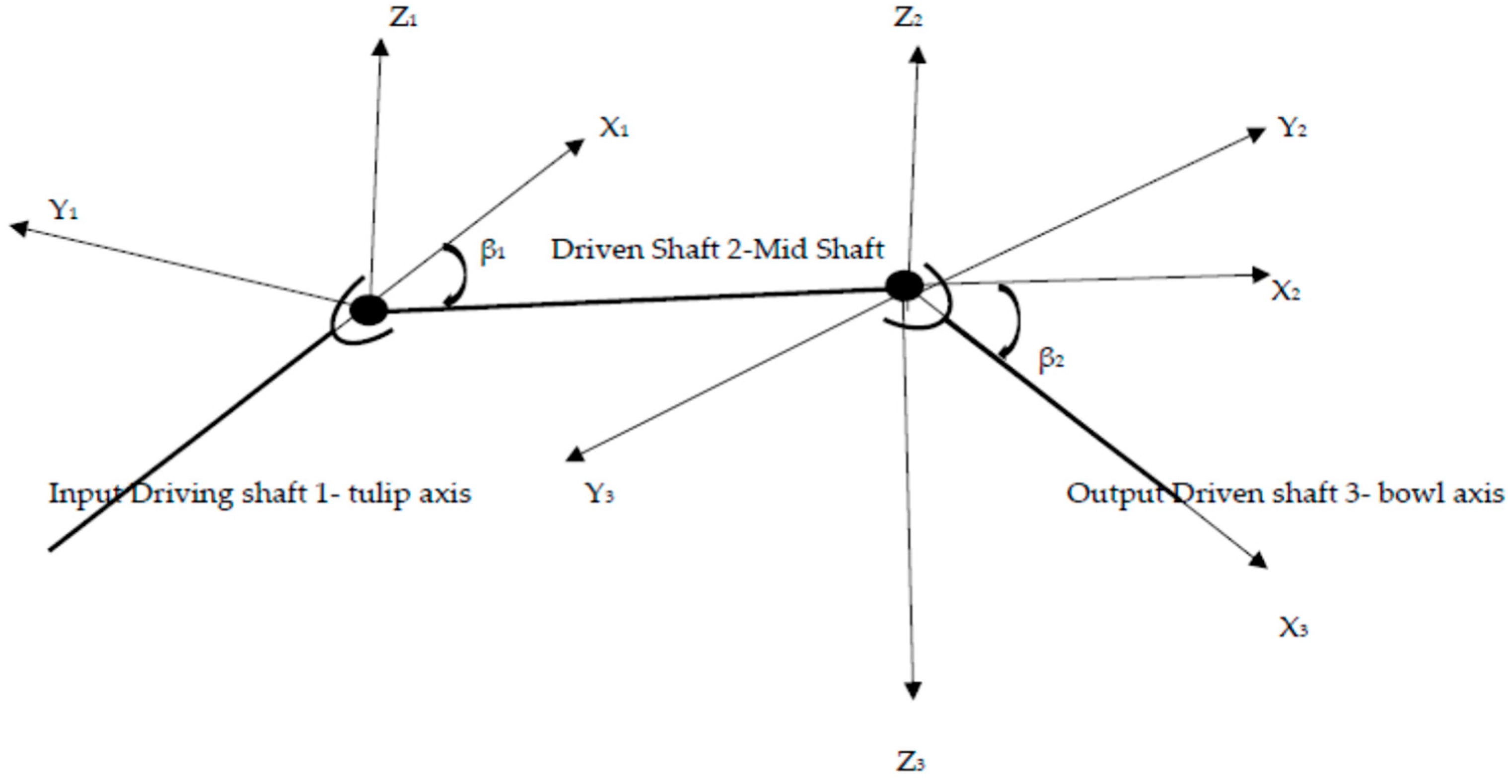
Presented in Figure 3 is the schematical representation of an automotive driveshaft in the three axes of Cartesian coordinates X₁Y₁Z₁ attached to the tulip, X₂Y₂Z₂ attached to the midshaft, and X₃Y₃Z₃ attached to the bowl, which having the following rigid movements:

-

rotation with the angle φ₁ of the tulip with respect to the axis X₁, φ₁ = 0 … n₁π;

-

rotation with the angle φ₂ of the mid shaft with respect to the axis X₂, φ₂ = 0 … n₁π;

-

rotation with the angle φ₃ of the bowl with respect to the axis X₃, φ₃ = 0 … n₁π;

-

relative rotation of the longitudinal axe of the midshaft (given by the direction of the axis X₂) with respect to the longitudinal direction of the tulip (given by the direction of the axis X₁), with β₁ (spatial angle between axis X₁ and X₂) with respect to the axis Z₁, β₁ being the angle between longitudinal direction of the tulip and the longitudinal direction of the midshaft, β₁ = 0° … 15°;

-

relative rotation of the longitudinal axis of the bowl (given by the direction of the axis X₃) with respect to the longitudinal direction of the midshaft (given by the direction of the axis X₂), with β₂ (spatial angle between axis X₂ and X₃) with respect to the axe Y₂, β₂ being the angle between the longitudinal direction of the midshaft and the longitudinal direction of the bowl, β₂ = 0° … 47°.

In Figure 3, it is considered that the axes (X₁, Y₁), (X₂, Y₂), and (X₃, Y₃) are in the same plane and, therefore, the axes Z₁, Z₂, Z₃ are parallel, and this supposition does not restrain generality.

The geometrical details of the tulip–tripod joint is presented in Figure 4, and the geometrical details of the bowl–balls joint are presented in Figure 5.

As can be seen from Figure 4, the tripod is fixed to the midshaft, the inner race is fixed to the midshaft (see Figure 5) and the car wheel is fixed to the bowl (see Figure 5).

2. Computation of the Mass Moments and Geometric Moments of Driveshaft Inertia

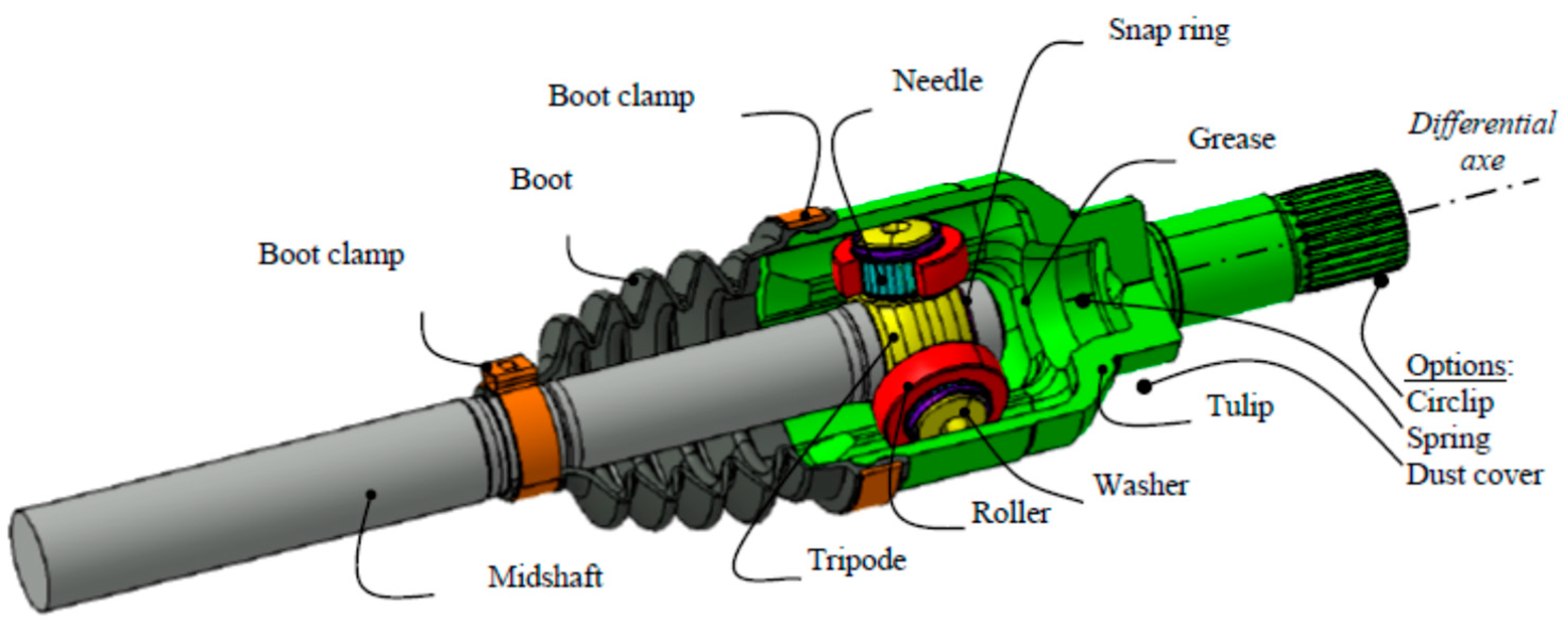
In order to compute the equations of motions for the driveshaft using the variational approach of Hamilton’s principle, it is necessary to reduce the axial mass moment of inertia of the cross section ${\mathrm{I}}_{{\mathrm{X}}_1\mathrm{G}\mathrm{T}}$ and the geometric moment of inertia of the cross section ${\mathrm{J}}_{{\mathrm{X}}_1\mathrm{G}\mathrm{T}}$ for the global tulip (tulip axis and tulip) with respect to the longitudinal axis of the midshaft X₂ in the centroid of the cross section of the tripod fixed on the midshaft (see Figure 4) as well as the axial mass moment of inertia of the cross section ${\mathrm{I}}_{{\mathrm{X}}_3\mathrm{G}\mathrm{B}}$ and the axial geometric moment of inertia of the cross section ${\mathrm{J}}_{{\mathrm{X}}_3\mathrm{G}\mathrm{B}}$ for the global bowl (bowl axis and bowl) with respect to the longitudinal axis of the midshaft X₂ in the centroid of the cross section of the inner race fixed on the midshaft (see Figure 5). The computations of these axial mass moments of inertia of the cross section and axial geometric moments of inertia of the cross section take the following into account: the angle β₁ between X₁ and X₂ (see Figure 3, rotation with respect to Z₁ parallel with Z₂), the distance from the mass center of the tulip axis to the centroid of the cross section of the tripod fixed on the midshaft, the distance from the mass center of the tulip to the centroid of the cross section of the tripod fixed on the midshaft (see Figure 4), the angle β₂ between X₂ and X₃ (see Figure 3, rotation with respect to Z₃ parallel with Z₂), the distance from the mass center of the bowl axis to the centroid of the cross section of inner race fixed on the midshaft, and the distance from the mass center of the bowl to the centroid of the cross section of inner race fixed on the midshaft (see Figure 5). In its design, the global tulip consists of two major parts, the tulip and tulip axis, as can be seen in Figure 4, which have different geometry and therefore different mass and geometric moments of inertia. Thus, it is obtained that the axial geometric moment of inertia of the cross section for the global tulip ${\mathrm{J}}_{{\mathrm{X}}_2\mathrm{G}\mathrm{T}}$ can be reduced to the longitudinal axis of the midshaft in the centroid of the cross section of the tripod fixed on the midshaft, and the axial mass moment of inertia of the cross section for the global tulip ${\mathrm{I}}_{{\mathrm{X}}_2\mathrm{G}\mathrm{T}}$ can be reduced to the longitudinal axis of the midshaft in the centroid of the cross section of the tripod fixed on the midshaft, given by the following equations:

$${\mathrm{J}}_{{\mathrm{X}}_2\mathrm{G}\mathrm{T}}={\mathrm{J}}_{{\mathrm{X}}_2\mathrm{T}}+{\mathrm{J}}_{{\mathrm{X}}_2\mathrm{A}\mathrm{T}},$$

(1)

$${\mathrm{J}}_{{\mathrm{X}}_2\mathrm{T}}=0.5\left({\mathrm{J}}_{1\mathrm{T}}+{\mathrm{J}}_{2\mathrm{T}}\right)\left[1+{\cos }^2{\mathsf{\beta }}_1+{\mathsf{\chi }}_{\mathrm{n}\mathrm{T}}\cos \left(2{\mathsf{\phi }}_1\right){\sin }^2{\mathsf{\beta }}_1\right]+{\mathrm{S}}_{\mathrm{T}}{\left({\mathrm{d}}_{\mathrm{C}\mathrm{T}}\right)}^2,$$

(2)

$${\mathsf{\chi }}_{\mathrm{n}\mathrm{T}}=\frac{{\mathrm{J}}_{1\mathrm{T}}-{\mathrm{J}}_{2\mathrm{T}}}{{\mathrm{J}}_{1\mathrm{T}}+{\mathrm{J}}_{2\mathrm{T}}},$$

(3)

$${\mathrm{J}}_{{\mathrm{X}}_2\mathrm{A}\mathrm{T}}=\frac{\mathsf{\pi }{\mathrm{d}}_{\mathrm{A}\mathrm{T}}^4}{64}\left(1+{\cos }^2{\mathsf{\beta }}_1\right)+\frac{\mathsf{\pi }{\mathrm{d}}_{\mathrm{A}\mathrm{T}}^2}{4}{\left({\mathrm{L}}_{\mathrm{T}}+0.5{\mathrm{L}}_{\mathrm{A}\mathrm{T}}\right)}^2,$$

(4)

$${\mathrm{I}}_{{\mathrm{X}}_2\mathrm{G}\mathrm{T}}={\mathrm{J}}_{{\mathrm{X}}_2\mathrm{T}}\mathsf{\rho }{\mathrm{L}}_{\mathrm{T}}+{\mathrm{J}}_{{\mathrm{X}}_2\mathrm{A}\mathrm{T}}\mathsf{\rho }{\mathrm{L}}_{\mathrm{A}\mathrm{T}},$$

(5)

where ${\mathrm{J}}_{1\mathrm{T}},{\mathrm{J}}_{2\mathrm{T}}$ are the principal geometric moments of inertia with respect to the cross section of the tulip in the center mass of the tulip, ${\mathrm{J}}_{{\mathrm{X}}_2\mathrm{T}},{\mathrm{J}}_{{\mathrm{X}}_2\mathrm{A}\mathrm{T}}$ are the geometric moment of inertia of the tulip and the geometric moment of inertia of the tulip axis reduced to the longitudinal axis of the midshaft in the centroid of the cross section of the tripod fixed on the midshaft, $\mathsf{\rho }$ is the volume mass density of the material of the driveshaft, ${\mathrm{d}}_{\mathrm{C}\mathrm{T}}$ is the distance between the center mass of the tulip and the centroid of the tripod, ${\mathrm{S}}_{\mathrm{T}}$ is the area cross section of the tulip, ${\mathsf{\chi }}_{\mathrm{n}\mathrm{T}}$ is the nonuniformity of the geometric moments of inertia in the cross section of the tulip (see Figure 4), ${\mathrm{L}}_{\mathrm{T}}$ is the length of the tulip, ${\mathrm{L}}_{\mathrm{A}\mathrm{T}}$ is the length of the tulip axis, d_AT is the diameter of the tulip axis and ${\mathsf{\phi }}_1$ is the angle of rotation of the tulip with respect to the axis X₁. In its design, the global bowl consists of two major parts, the bowl and bowl axis (wheel axis), as can be seen in Figure 5, which have different geometry and therefore different mass and geometric moments of inertia. In the same mathematical manner, ${\mathrm{J}}_{{\mathrm{X}}_2\mathrm{G}\mathrm{B}}$ is obtained, which is the axial geometric moment of inertia of the cross section for the global bowl reduced to the longitudinal axis of the midshaft in the centroid of the cross section of the inner race fixed on the midshaft (see Figure 5), as is ${\mathrm{I}}_{{\mathrm{X}}_2\mathrm{G}\mathrm{B}}$, the axial mass moment of inertia of the cross section for the global bowl reduced to the longitudinal axis of the midshaft in the centroid of the cross section of the inner race fixed on the midshaft, given by these equations:

$${\mathrm{J}}_{{\mathrm{X}}_2\mathrm{G}\mathrm{B}}={\mathrm{J}}_{{\mathrm{X}}_2\mathrm{B}}+{\mathrm{J}}_{{\mathrm{X}}_2\mathrm{A}\mathrm{B}},$$

(6)

$${\mathrm{J}}_{{\mathrm{X}}_2\mathrm{B}}=0.5\left({\mathrm{J}}_{1\mathrm{B}}+{\mathrm{J}}_{2\mathrm{B}}\right)\left[1+{\cos }^2{\mathsf{\beta }}_2+{\mathsf{\chi }}_{\mathrm{n}\mathrm{B}}\cos \left(2{\mathsf{\phi }}_3\right){\sin }^2{\mathsf{\beta }}_2\right]+{\mathrm{S}}_{\mathrm{B}}{\left({\mathrm{d}}_{\mathrm{C}\mathrm{B}}\right)}^2,$$

(7)

$${\mathsf{\chi }}_{\mathrm{n}\mathrm{B}}=\frac{{\mathrm{J}}_{1\mathrm{B}}-{\mathrm{J}}_{2\mathrm{B}}}{{\mathrm{J}}_{1\mathrm{B}}+{\mathrm{J}}_{2\mathrm{B}}},$$

(8)

$${\mathrm{J}}_{{\mathrm{X}}_2\mathrm{A}\mathrm{B}}=\frac{\mathsf{\pi }{\mathrm{d}}_{\mathrm{A}\mathrm{B}}^4}{64}\left(1+{\cos }^2{\mathsf{\beta }}_1\right)+\frac{\mathsf{\pi }{\mathrm{d}}_{\mathrm{A}\mathrm{B}}^2}{4}{\left({\mathrm{L}}_{\mathrm{B}}+0.5{\mathrm{L}}_{\mathrm{A}\mathrm{B}}\right)}^2,$$

(9)

$${\mathrm{I}}_{{\mathrm{X}}_2\mathrm{G}\mathrm{B}}={\mathrm{J}}_{{\mathrm{X}}_2\mathrm{B}}\mathsf{\rho }{\mathrm{L}}_{\mathrm{B}}+{\mathrm{J}}_{{\mathrm{X}}_2\mathrm{A}\mathrm{B}}\mathsf{\rho }{\mathrm{L}}_{\mathrm{A}\mathrm{B}},$$

(10)

where ${\mathrm{J}}_{1\mathrm{B}},{\mathrm{J}}_{2\mathrm{B}}$ are the principal geometric moments of inertia with respect to the cross section of the bowl in the center mass of the bowl; ${\mathrm{J}}_{{\mathrm{X}}_2\mathrm{B}},{\mathrm{J}}_{{\mathrm{X}}_2\mathrm{A}\mathrm{B}}$ are the geometric moment of inertia of the bowl and the geometric moment of inertia of the bowl axis reduced to the longitudinal axis of the midshaft in the centroid of the cross section of the inner race fixed on the midshaft, respectively; $\mathsf{\rho }$ is the volume mass density of the driveshaft material; ${\mathrm{d}}_{\mathrm{C}\mathrm{B}}$ is the distance between the center mass of the bowl and the centroid of the inner race; ${\mathrm{S}}_{\mathrm{B}}$ is the area cross section of the bowl; ${\mathsf{\chi }}_{\mathrm{n}\mathrm{B}}$ is the nonuniformity of the geometric moments of inertia in the cross section of the bowl (see Figure 4); ${\mathrm{L}}_{\mathrm{B}}$ is the length of the bowl; ${\mathrm{L}}_{\mathrm{A}\mathrm{B}}$ is the length of the bowl axis; d_AB is the diameter of the bowl axis; and ${\mathsf{\phi }}_3$ is the angle of rotation of the tulip with respect to the axis X₃. As can be seen analyzing Equations (1)–(10), the geometric axial moment of inertia of the cross section ${\mathrm{J}}_{{\mathrm{X}}_2\mathrm{G}\mathrm{T}}$, for the global tulip, and the geometric axial moment of inertia of the cross section ${\mathrm{J}}_{{\mathrm{X}}_2\mathrm{G}\mathrm{B}}$, for the global bowl, both reduced to the longitudinal midshaft axis X₂, are functions that contains the effects o: twisting angle of tulip ${\mathsf{\phi }}_1$ as well as the twisting angle of bowl ${\mathsf{\phi }}_3$, nonuniformity of the geometric moments of inertia of the cross section for both tulip and bowl ${\mathsf{\chi }}_{\mathrm{n}\mathrm{T}}$ and ${\mathsf{\chi }}_{\mathrm{n}\mathrm{B}}$, the angle between longitudinal direction of the tulip and the longitudinal direction of the midshaft ${\mathsf{\beta }}_1$, the angle between the longitudinal direction of the midshaft and the longitudinal direction of the bowl ${\mathsf{\beta }}_2$, the length of the tulip and the length of the bowl, the position of the mass center of the tulip axis and tulip with respect to the centroid of the tripod, the position of the mass center of the bowl axis and bowl with respect to the centroid of the inner race, the principal geometric moments of inertia of the cross section for the tulip ${\mathrm{J}}_{1\mathrm{T}},{\mathrm{J}}_{2\mathrm{T}}$, the principal geometric moments of inertia of the cross section for the bowl ${\mathrm{J}}_{1\mathrm{B}},{\mathrm{J}}_{2\mathrm{B}}$, d_AT the diameter of the tulip axis, and d_AB the diameter of the bowl axis.

3. The Physical Model of the Driveshaft in Torsion

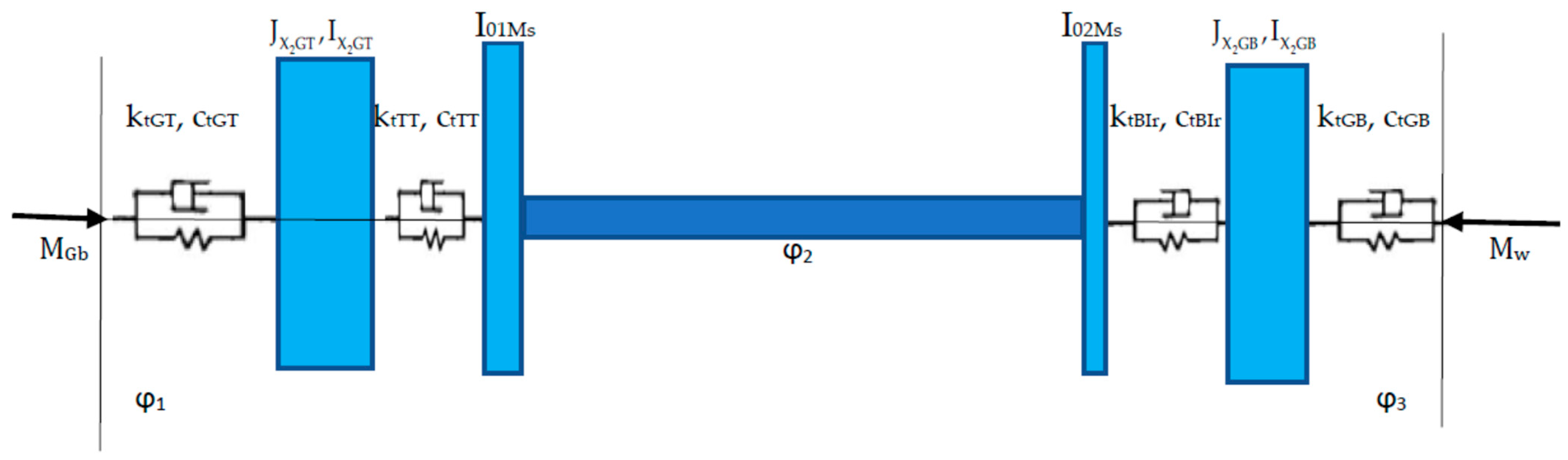
The physical model for torsional vibrations of the driveshaft is presented in Figure 6.

The present model (see Figure 6) considers that the tulip (see Figure 4) and the bowl (see Figure 5) have rigid body torsion movements, through the twist angles ${\mathsf{\phi }}_1$ and ${\mathsf{\phi }}_3$, that are functions of time ${\mathsf{\phi }}_1={\mathsf{\phi }}_1\left(\mathrm{t}\right)$ and ${\mathsf{\phi }}_3={\mathsf{\phi }}_3\left(\mathrm{t}\right)$, while the midshaft has a twist angle ${\mathsf{\phi }}_2$ that is a function ${\mathsf{\phi }}_2={\mathsf{\phi }}_2\left(\mathrm{x},\mathrm{t}\right)$ of position (space) in the longitudinal direction of the midshaft, where $\mathrm{x}\in \left[0,{\mathrm{L}}_{\mathrm{M}\mathrm{s}}\right],{\mathrm{L}}_{\mathrm{M}\mathrm{s}}$ being the length of the midshaft of the automotive driveshaft (see Figure 2), and the time t. The effect of nonuniformity for the geometric and kinematic isometry of the driveshaft [1,4] is given by the equations:

$${\mathsf{\phi }}_2\left(0,\mathrm{t}\right)={\mathsf{\phi }}_1\left(\mathrm{t}\right)+\frac{{\mathrm{R}}_{\mathrm{T}\mathrm{T}\mathrm{r}}}{2{\mathrm{L}}_{\mathrm{M}\mathrm{s}}}\tan {\mathsf{\beta }}_1{\tan }^2\frac{{\mathsf{\beta }}_1}{2}\cos (3{\mathsf{\phi }}_1),$$

(11)

$${\mathsf{\phi }}_3\left(\mathrm{t}\right)={\mathsf{\phi }}_2\left({\mathrm{L}}_{\mathrm{M}\mathrm{s}},\mathrm{t}\right)+\frac{{\mathrm{R}}_{\mathrm{I}\mathrm{r}\mathrm{B}}}{2{\mathrm{L}}_{\mathrm{M}\mathrm{s}}}\tan {\mathsf{\beta }}_2{\tan }^2\frac{{\mathsf{\beta }}_2}{2}\cos (3{\mathsf{\phi }}_2\left({\mathrm{L}}_{\mathrm{M}\mathrm{s}},\mathrm{t}\right)),$$

(12)

where ${\mathrm{R}}_{\mathrm{T}\mathrm{T}\mathrm{r}}$ is the tulip–tripod joint radius (see Figure 4) and ${\mathrm{R}}_{\mathrm{I}\mathrm{r}\mathrm{B}}$ is the inner race-bowl joint radius (see Figure 5). Deriving the Equations (11) and (12) with respect to time yields:

$$\frac{\partial {\mathsf{\phi }}_2\left(0,\mathrm{t}\right)}{\partial \mathrm{t}}-{\stackrel{•}{\mathsf{\phi }}}_1\left(\mathrm{t}\right)=-{1.5}_1{\stackrel{•}{\mathsf{\phi }}}_1\left(\mathrm{t}\right)\frac{{\mathrm{R}}_{\mathrm{T}\mathrm{T}\mathrm{r}}}{{\mathrm{L}}_{\mathrm{M}\mathrm{s}}}\tan {\mathsf{\beta }}_1{\tan }^2\frac{{\mathsf{\beta }}_1}{2}\sin (3{\mathsf{\phi }}_1),$$

(13)

$${\stackrel{•}{\mathsf{\phi }}}_3\left(\mathrm{t}\right)-\frac{\partial {\mathsf{\phi }}_2\left({\mathrm{L}}_{\mathrm{M}\mathrm{s}},\mathrm{t}\right)}{\partial \mathrm{t}}=-{1.5}_1\frac{\partial {\mathsf{\phi }}_2\left({\mathrm{L}}_{\mathrm{M}\mathrm{s}},\mathrm{t}\right)}{\partial \mathrm{t}}\frac{{\mathrm{R}}_{\mathrm{T}\mathrm{T}\mathrm{r}}}{{\mathrm{L}}_{\mathrm{M}\mathrm{s}}}\tan {\mathsf{\beta }}_2{\tan }^2\frac{{\mathsf{\beta }}_2}{2}\sin (3{\mathsf{\phi }}_2\left({\mathrm{L}}_{\mathrm{M}\mathrm{s}},\mathrm{t}\right)).$$

(14)

Equations (11)–(14) introduce, in this model, the effect of nonuniformity for the geometric and kinematic isometry of the automotive driveshaft [1,4]. The model presented consists of three different elements, tulip–midshaft–bowl, linked through two links the joint tulip–tripod (mounted on the midshaft, see Figure 4), and the joint bowl–balls–inner race (mounted at the other edge of the midshaft, see Figure 5), described in terms of dynamic torsion as follows:

• the tulip in torsional rigid body movement reduced to the torsional longitudinal axis of the midshaft, having a global torsional stiffness ${\mathrm{k}}_{\mathrm{t}\mathrm{G}\mathrm{T}}$, a global torsional damping coefficient ${\mathrm{c}}_{\mathrm{t}\mathrm{G}\mathrm{T}}$, an axial geometric moment of inertia of the cross section for the global tulip ${\mathrm{J}}_{{\mathrm{X}}_2\mathrm{G}\mathrm{T}}$ reduced to the longitudinal axis of the midshaft in the centroid of the cross section of tripode fixed on the midshaft (see Equation (1)), an axial mass moment of inertia of the cross section for the global tulip ${\mathrm{I}}_{{\mathrm{X}}_2\mathrm{G}\mathrm{T}}$ reduced to the longitudinal axis of the midshaft in the centroid of the cross section of tripode fixed on the midshaft (see Equation (5)), where ${\mathrm{k}}_{\mathrm{t}\mathrm{G}\mathrm{T}}$ and ${\mathrm{c}}_{\mathrm{t}\mathrm{G}\mathrm{T}}$ are given by the equations:

  $${\mathrm{k}}_{\mathrm{t}\mathrm{G}\mathrm{T}}=\frac{{\mathrm{k}}_{\mathrm{t}\mathrm{A}\mathrm{T}}{\mathrm{k}}_{\mathrm{t}\mathrm{T}}}{{\mathrm{k}}_{\mathrm{t}\mathrm{A}\mathrm{T}}+{\mathrm{k}}_{\mathrm{t}\mathrm{T}}},{\mathrm{k}}_{\mathrm{t}\mathrm{A}\mathrm{T}}=\frac{\mathrm{G}{\mathrm{J}}_{{\mathrm{X}}_2\mathrm{A}\mathrm{T}}}{{\mathrm{L}}_{\mathrm{A}\mathrm{T}}},{\mathrm{k}}_{\mathrm{t}\mathrm{T}}=\frac{\mathrm{G}{\mathrm{J}}_{{\mathrm{X}}_2\mathrm{T}}}{{\mathrm{L}}_{\mathrm{T}}},{\mathrm{c}}_{\mathrm{t}\mathrm{G}\mathrm{T}}=\frac{2{\Delta }_{\mathrm{G}\mathrm{T}}}{\sqrt{4{\mathsf{\pi }}^2+{\Delta }_{\mathrm{G}\mathrm{T}}^2}}\sqrt{{\mathrm{k}}_{\mathrm{t}\mathrm{G}\mathrm{T}}{\mathrm{I}}_{{\mathrm{X}}_2\mathrm{G}\mathrm{T}}},$$

  (15)

  where ${\mathrm{k}}_{\mathrm{t}\mathrm{A}\mathrm{T}}$ is the stiffness/rigidity of the tulip axis reduced to the longitudinal axis of the midshaft in the centroid of the cross section of the tripod fixed on the midshaft, ${\mathrm{k}}_{\mathrm{t}\mathrm{T}}$ is the stiffness/rigidity of the tulip reduced to the longitudinal axis of the midshaft in the centroid of the cross section of the tripod fixed on the midshaft, ${\mathrm{L}}_{\mathrm{T}}$ is the length of the tulip, ${\mathrm{L}}_{\mathrm{A}\mathrm{T}}$ is the length of the tulip axis, G is the shear modulus, and ${\Delta }_{\mathrm{G}\mathrm{T}}$ is the logarithmic decrement of the free torsional vibrations of the global tulip (${\Delta }_{\mathrm{G}\mathrm{T}}=0.001\dots 0.2$) [20,21];
• The joint tulip–tripod in torsion realizes the link between the tulip and the midshaft through the torsional stiffness ${\mathrm{k}}_{\mathrm{t}\mathrm{T}\mathrm{T}}$ and the damping torsional coefficient ${\mathrm{c}}_{\mathrm{t}\mathrm{T}\mathrm{T}}$;
• The uniform midshaft (see Figure 2, Figure 4, and Figure 5) in torsion having, at x = 0, a tripod (see Figure 4) fixed on the midshaft with the axial mass moment of inertia of the cross section ${\mathrm{I}}_{01\mathrm{M}\mathrm{s}}$ (midshaft axis included on the thickness of the tripod) and the geometric axial moment of inertia of the cross section of the tripod ${\mathrm{J}}_{{\mathrm{X}}_2\mathrm{T}\mathrm{r}}$ (midshaft axis included on the thickness of the tripod), and at $\mathrm{x}={\mathrm{L}}_{\mathrm{M}\mathrm{s}}$, an inner race (see Figure 5) fixed on the midshaft with the axial mass moment of inertia of the cross section ${\mathrm{I}}_{02\mathrm{M}\mathrm{s}}$ (midshaft axis included on the thickness of the inner race) and the geometric axial moment of inertia of the cross section ${\mathrm{J}}_{{\mathrm{X}}_2\mathrm{I}\mathrm{r}}$ (midshaft axis included on the thickness of the inner race), given by the equations:

  $${\mathrm{I}}_{01\mathrm{M}\mathrm{s}}={\mathrm{J}}_{{\mathrm{X}}_2\mathrm{T}\mathrm{r}}\mathsf{\rho }{\mathrm{L}}_{\mathrm{T}\mathrm{r}}=\left({\mathrm{J}}_{1\mathrm{T}\mathrm{r}}+{\mathrm{J}}_{2\mathrm{T}\mathrm{r}}\right)\mathsf{\rho }{\mathrm{L}}_{\mathrm{T}\mathrm{r}},$$

  (16)

  $${\mathrm{I}}_{02\mathrm{M}\mathrm{s}}={\mathrm{J}}_{{\mathrm{X}}_2\mathrm{I}\mathrm{r}}\mathsf{\rho }{\mathrm{L}}_{\mathrm{I}\mathrm{r}}=\left({\mathrm{J}}_{1\mathrm{I}\mathrm{r}}+{\mathrm{J}}_{2\mathrm{I}\mathrm{r}}\right)\mathsf{\rho }{\mathrm{L}}_{\mathrm{I}\mathrm{r}},$$

  (17)

  where ${\mathrm{J}}_{1\mathrm{T}\mathrm{r}},{\mathrm{J}}_{2\mathrm{T}\mathrm{r}}$ are the principal geometric moments of inertia in the cross section of the tripod, midshaft axis included on the thickness of the tripod, ${\mathrm{J}}_{1\mathrm{I}\mathrm{r}},{\mathrm{J}}_{2\mathrm{I}\mathrm{r}}$ are the principal geometric moments of inertia in the cross section of the inner race, midshaft axis included on the thickness of the inner race, ${\mathrm{J}}_{{\mathrm{X}}_2\mathrm{T}\mathrm{r}}$ is the geometric axial moment of inertia of the tripod (midshaft axis included on the thickness of the tripod), ${\mathrm{J}}_{{\mathrm{X}}_2\mathrm{I}\mathrm{r}}$ is the geometric axial moment of inertia of the inner race (midshaft axis included on the thickness of the inner race), ${\mathrm{L}}_{\mathrm{T}\mathrm{r}}$ is the thickness of the tripod, ${\mathrm{L}}_{\mathrm{I}\mathrm{r}}$ is the thickness of the inner race;
• The joint bowl–balls–inner race in torsion realizes the link between the bowl and the midshaft through the torsional stiffness k_tBIr and the damping torsional coefficient c_tBIr;
• The bowl in torsional rigid body movement is reduced to the torsional longitudinal axis of the midshaft, having a global torsional stiffness ${\mathrm{k}}_{\mathrm{t}\mathrm{G}\mathrm{B}}$, a global torsional damping coefficient ${\mathrm{c}}_{\mathrm{t}\mathrm{G}\mathrm{B}}$, an axial geometric moment of inertia of the cross section reduced to the longitudinal axe of the midshaft J_X2GB (see Equation (6), an axial mass moment of inertia of the cross section reduced to the longitudinal axe of the midshaft ${\mathrm{I}}_{{\mathrm{X}}_2\mathrm{G}\mathrm{B}}$ (see Equation (10)), where ${\mathrm{k}}_{\mathrm{t}\mathrm{G}\mathrm{B}}$ and ${\mathrm{c}}_{\mathrm{t}\mathrm{G}\mathrm{B}}$ are given by the equations:

  $${\mathrm{k}}_{\mathrm{t}\mathrm{G}\mathrm{B}}=\frac{{\mathrm{k}}_{\mathrm{t}\mathrm{A}\mathrm{B}}{\mathrm{k}}_{\mathrm{t}\mathrm{B}}}{{\mathrm{k}}_{\mathrm{t}\mathrm{A}\mathrm{B}}+{\mathrm{k}}_{\mathrm{t}\mathrm{B}}},{\mathrm{k}}_{\mathrm{t}\mathrm{A}\mathrm{T}}=\frac{\mathrm{G}{\mathrm{J}}_{{\mathrm{X}}_2\mathrm{A}\mathrm{B}}}{{\mathrm{L}}_{\mathrm{A}\mathrm{B}}},{\mathrm{k}}_{\mathrm{t}\mathrm{T}}=\frac{\mathrm{G}{\mathrm{J}}_{{\mathrm{X}}_2\mathrm{B}}}{{\mathrm{L}}_{\mathrm{B}}},{\mathrm{c}}_{\mathrm{t}\mathrm{G}\mathrm{B}}=\frac{2{\Delta }_{\mathrm{G}\mathrm{B}}}{\sqrt{4{\mathsf{\pi }}^2+{\Delta }_{\mathrm{G}\mathrm{B}}^2}}\sqrt{{\mathrm{k}}_{\mathrm{t}\mathrm{G}\mathrm{B}}{\mathrm{I}}_{{\mathrm{X}}_2\mathrm{G}\mathrm{B}}},$$

  (18)

  where ${\mathrm{k}}_{\mathrm{t}\mathrm{A}\mathrm{B}}$ is the stiffness/rigidity of the bowl axis reduced to the longitudinal axis of the midshaft in the centroid of the cross section of the inner race fixed on the midshaft, ${\mathrm{k}}_{\mathrm{t}\mathrm{B}}$ is the stiffness/rigidity of the bowl reduced to the longitudinal axis of the midshaft in the centroid of the cross section of the inner race fixed on the midshaft, ${\mathrm{L}}_{\mathrm{B}}$ is the length of the bowl, ${\mathrm{L}}_{\mathrm{A}\mathrm{B}}$ is the length of the bowl axis, G is the shear modulus and ${\Delta }_{\mathrm{G}\mathrm{B}}$ the logarithmic decrement of the free torsional vibrations of the global bowl (Δ_GB = 0.001–0.15) [20,21].

From the gearbox, the driveshaft (see Figure 1 and Figure 6) receives torque from the engine that is given by Equation (2) (p. 361)

$${\mathrm{M}}_{\mathrm{G}\mathrm{b}}={\overline{\mathrm{M}}}_{\mathrm{e}}\left[1+{\mathsf{\chi }}_{\mathrm{e}}\cos \left(\mathrm{n}{\Omega }_{\mathrm{e}}\mathrm{t}\right)\right],\mathrm{n}\in \mathrm{N},$$

(19)

$${\Omega }_{\mathrm{e}}=\frac{\mathsf{\pi }{\mathrm{n}}_{\mathrm{e}}}{30},$$

(20)

where ${\mathsf{\chi }}_{\mathrm{e}}$ is the nonuniformity of the internal engine torque, being in the range 0.980–1.020 [2] (p. 363) and ${\overline{\mathrm{M}}}_{\mathrm{e}}$ is the amplitude of the engine torque in Nm and ${\mathrm{n}}_{\mathrm{e}}$ is the speed rotation (velocity angle) of the crank shaft of the engine in rot/min. The reactive torque induced by the wheel is a moderate impulsive type and can be considered in the mathematical form

$${\mathrm{M}}_{\mathrm{w}}={\mathrm{M}}_{\mathrm{H}}\left[1+{\mathrm{q}}_3{\mathrm{t}}^{{\mathrm{q}}_1}{\mathrm{e}}^{-{\mathrm{q}}_2\mathrm{t}}\right],$$

(21)

where ${\mathrm{M}}_{\mathrm{H}}$ is the adhesion torque [22] (p. 130), ${\mathrm{q}}_{\mathrm{i}},\mathrm{i}=\overline{1,3},{\mathrm{q}}_1\gg {\mathrm{q}}_2,{\mathrm{q}}_3\ge 1.1$ are experimental constants depending on the type of shock applied at the wheel by the road excitation [3].

4. The Equations of Forced Torsional Vibrations of the Automotive Driveshaft

For the model of torsional vibrations of the automotive driveshaft presented in Figure 6, use of the variational approach of the generalized Hamilton’s principle [23] (pp. 272–295) yields

$$\mathsf{\delta }{\displaystyle \underset{{\mathrm{t}}_1}{\overset{{\mathrm{t}}_2}{\int }}\left(\Pi -\mathrm{T}-\mathrm{W}\right)\mathrm{d}\mathrm{t}=0,}$$

(22)

where the strain energy $\Pi$ of the model for the automotive driveshaft (see Figure 6), including the torsional springs and the torsional dampers, is given by the generalized Equation (23) (p. 274), [24] (pp. 610–613):

$$\begin{gathered} \Pi =\frac{1}{2}{\displaystyle \underset{0}{\overset{{\mathrm{L}}_{\mathrm{M}\mathrm{s}}}{\int }}\mathrm{G}{\mathrm{J}}_{{\mathrm{X}}_2\mathrm{M}\mathrm{s}}{\left(\frac{\partial {\mathsf{\phi }}_2}{\partial \mathrm{x}}\right)}^2}\mathrm{d}\mathrm{x}+\frac{1}{2}\left[{\mathrm{c}}_{\mathrm{t}\mathrm{G}\mathrm{T}}{\left(\stackrel{•}{{\mathsf{\phi }}_1}\right)}^2+{\mathrm{c}}_{\mathrm{t}\mathrm{T}\mathrm{T}}{\left(\frac{\partial {\mathsf{\phi }}_2\left(0,\mathrm{t}\right)}{\partial \mathrm{x}}-\stackrel{•}{{\mathsf{\phi }}_1}\right)}^2+{\mathrm{c}}_{\mathrm{t}\mathrm{B}\mathrm{I}\mathrm{r}}{\left(\stackrel{•}{{\mathsf{\phi }}_3}-\frac{\partial {\mathsf{\phi }}_2\left({\mathrm{L}}_{\mathrm{M}\mathrm{s}},\mathrm{t}\right)}{\partial \mathrm{x}}\right)}^2+{\mathrm{c}}_{\mathrm{t}\mathrm{G}\mathrm{B}}{\left(\stackrel{•}{{\mathsf{\phi }}_3}\right)}^2\right]+ \\ +\frac{1}{2}\left[{\mathrm{k}}_{\mathrm{t}\mathrm{G}\mathrm{T}}{\mathsf{\phi }}_1^2+{\mathrm{k}}_{\mathrm{t}\mathrm{T}\mathrm{T}}{\left({\mathsf{\phi }}_2\left(0,\mathrm{t}\right)-{\mathsf{\phi }}_1\right)}^2+{\mathrm{k}}_{\mathrm{t}\mathrm{B}\mathrm{I}\mathrm{r}}{\left({\mathsf{\phi }}_3-{\mathsf{\phi }}_2\left({\mathrm{L}}_{\mathrm{M}\mathrm{s}},\mathrm{t}\right)\right)}^2+{\mathrm{k}}_{\mathrm{t}\mathrm{G}\mathrm{B}}{\mathsf{\phi }}_3^2\right], \end{gathered}$$

(23)

where ${\mathrm{L}}_{\mathrm{M}\mathrm{s}}$ is the midshaft length, ${\mathrm{J}}_{{\mathrm{X}}_2\mathrm{M}\mathrm{s}}$ is the geometric axial moment of inertia of the cross section of the midshaft with respect to the longitudinal axis X₂ given by the equations

$${\mathrm{J}}_{{\mathrm{X}}_2\mathrm{M}\mathrm{s}}=\frac{\mathsf{\pi }{\mathrm{d}}_{\mathrm{M}\mathrm{s}}^4}{32},$$

(24)

$${\mathrm{J}}_{{\mathrm{X}}_2\mathrm{M}\mathrm{s}}=\frac{\mathsf{\pi }\left({\mathrm{d}}_{\mathrm{e}\mathrm{M}\mathrm{s}}^4-{\mathrm{d}}_{\mathrm{i}\mathrm{M}\mathrm{s}}^4\right)}{32},$$

(25)

where the midshaft is considered as having a circular or a tubular uniform cross section with the diameter ${\mathrm{d}}_{\mathrm{M}\mathrm{s}}$ for the circular cross section or the diameters ${\mathrm{d}}_{\mathrm{e}\mathrm{M}\mathrm{s}},{\mathrm{d}}_{\mathrm{i}\mathrm{M}\mathrm{s}}$ for the tubular cross section. Added to Equation (23) was the generalized Rayleigh’s dissipation function [24] (p. 611) specific to the mathematical formulations of the Euler–Lagrange generalized approach, due to the presence in the torsional vibration model of the damper, giving the equation

$$\Lambda \left(\stackrel{•}{{\mathsf{\phi }}_1},\frac{\partial {\mathsf{\phi }}_2\left(\mathrm{x},\mathrm{t}\right)}{\partial \mathrm{x}},\stackrel{•}{{\mathsf{\phi }}_3}\right)=\frac{1}{2}\left[{\mathrm{c}}_{\mathrm{t}\mathrm{G}\mathrm{T}}{\left(\stackrel{•}{{\mathsf{\phi }}_1}\right)}^2+{\mathrm{c}}_{\mathrm{t}\mathrm{T}\mathrm{T}}{\left(\frac{\partial {\mathsf{\phi }}_2\left(0,\mathrm{t}\right)}{\partial \mathrm{x}}-\stackrel{•}{{\mathsf{\phi }}_1}\right)}^2+{\mathrm{c}}_{\mathrm{t}\mathrm{B}\mathrm{I}\mathrm{r}}{\left(\stackrel{•}{{\mathsf{\phi }}_3}-\frac{\partial {\mathsf{\phi }}_2\left({\mathrm{L}}_{\mathrm{M}\mathrm{s}},\mathrm{t}\right)}{\partial \mathrm{x}}\right)}^2+{\mathrm{c}}_{\mathrm{t}\mathrm{G}\mathrm{B}}{\left(\stackrel{•}{{\mathsf{\phi }}_3}\right)}^2\right].$$

(26)

The kinetic energy of the model for the automotive driveshaft, seen in Figure 6, is given by the generalized Equation (23) (p. 274), [24] (p. 719):

$$\mathrm{T}={{\displaystyle \underset{0}{\overset{{\mathrm{L}}_{\mathrm{M}\mathrm{s}}}{\int }}\frac{1}{2}\mathsf{\rho }{\mathrm{J}}_{{\mathrm{X}}_2\mathrm{M}\mathrm{s}}\left(\frac{\partial {\mathsf{\phi }}_2}{\partial \mathrm{t}}\right)}}^2\mathrm{d}\mathrm{x}+\frac{1}{2}{\mathrm{I}}_{{\mathrm{X}}_2\mathrm{G}\mathrm{T}}{\left(\stackrel{•}{{\mathsf{\phi }}_1}\right)}^2+\frac{1}{2}{\mathrm{I}}_{01\mathrm{M}\mathrm{s}}{\left(\frac{\partial {\mathsf{\phi }}_2\left(0,\mathrm{t}\right)}{\partial \mathrm{t}}\right)}^2+\frac{1}{2}{\mathrm{I}}_{02\mathrm{M}\mathrm{s}}{\left(\frac{\partial {\mathsf{\phi }}_2\left({\mathrm{L}}_{\mathrm{M}\mathrm{s}},\mathrm{t}\right)}{\partial \mathrm{t}}\right)}^2+\frac{1}{2}{\mathrm{I}}_{{\mathrm{X}}_2\mathrm{G}\mathrm{B}}{\left(\stackrel{•}{{\mathsf{\phi }}_1}\right)}^2.$$

(27)

The work performed by the external torques can be expressed as

$$\mathrm{W}={\displaystyle {\int }_0^{{\mathrm{L}}_{\mathrm{M}\mathrm{s}}}\left\{\left[{\mathrm{M}}_{\mathrm{G}\mathrm{b}}\right]\Delta (\mathrm{x})+\left[{\mathrm{M}}_{\mathrm{w}}\right]\Delta (\mathrm{x}-{\mathrm{L}}_{\mathrm{M}\mathrm{s}})\right\}}{\mathsf{\phi }}_2(\mathrm{x},\mathrm{t})\mathrm{d}\mathrm{x}=\left[{\mathrm{M}}_{\mathrm{G}\mathrm{b}}\right]{\mathsf{\phi }}_2(0,\mathrm{t})+\left[{\mathrm{M}}_{\mathrm{w}}\right]{\mathsf{\phi }}_2({\mathrm{L}}_{\mathrm{M}\mathrm{s}},\mathrm{t}),$$

(28)

where $\Delta (\mathrm{x})$ is the Dirac’s function and ${\mathsf{\phi }}_2(0,\mathrm{t})$, ${\mathsf{\phi }}_2({\mathrm{L}}_{\mathrm{M}\mathrm{s}},\mathrm{t})$ are given by the Equations (11) and (12) as functions of ${\mathsf{\phi }}_1(\mathrm{t})$ and ${\mathsf{\phi }}_3(\mathrm{t})$. After several mathematical manipulations that include integration by parts, the nonlinear system with partial derivatives of second degree is yielded:

$${\mathrm{I}}_{{\mathrm{X}}_2\mathrm{G}\mathrm{T}}({\mathsf{\phi }}_1){\ddot{\mathsf{\phi }}}_1+\left[{\mathrm{c}}_{\mathrm{t}\mathrm{G}\mathrm{T}}+3{\mathrm{c}}_{\mathrm{t}\mathrm{T}\mathrm{T}}{\mathrm{A}}_{\mathrm{T}\mathrm{T}\mathrm{r}}\sin (3{\mathsf{\phi }}_1)\right]{\dot{\mathsf{\phi }}}_1+\left[{\mathrm{k}}_{\mathrm{t}\mathrm{G}\mathrm{T}}-{\mathrm{k}}_{\mathrm{t}\mathrm{T}\mathrm{T}}{\mathrm{A}}_{\mathrm{T}\mathrm{T}\mathrm{r}}\cos (3{\mathsf{\phi }}_1)\right]{\mathsf{\phi }}_1={\overline{\mathrm{M}}}_{\mathrm{e}}\left[1+{\mathsf{\chi }}_{\mathrm{e}}\cos \left(\mathrm{n}{\Omega }_{\mathrm{e}}\mathrm{t}\right)\right]\left(1-3{\mathrm{A}}_{\mathrm{T}\mathrm{T}\mathrm{r}}\sin (3{\mathsf{\phi }}_1)\right),$$

(29)

$$\mathsf{\rho }{\mathrm{J}}_{{\mathrm{X}}_2\mathrm{M}\mathrm{s}}\frac{{\partial }^2{\mathsf{\phi }}_2}{\partial {\mathrm{t}}^2}=\mathrm{G}{\mathrm{J}}_{{\mathrm{X}}_2\mathrm{M}\mathrm{s}}\frac{{\partial }^2{\mathsf{\phi }}_2}{\partial {\mathrm{x}}^2},$$

(30)

$${\mathrm{I}}_{{\mathrm{X}}_2\mathrm{G}\mathrm{B}}({\mathsf{\phi }}_3){\ddot{\mathsf{\phi }}}_3+\left[{\mathrm{c}}_{\mathrm{t}\mathrm{G}\mathrm{B}}-3{\mathrm{c}}_{\mathrm{t}\mathrm{B}\mathrm{I}\mathrm{r}}{\mathrm{A}}_{\mathrm{B}\mathrm{I}\mathrm{r}}\sin (3{\mathsf{\phi }}_3)\right]{\dot{\mathsf{\phi }}}_3+\left[{\mathrm{k}}_{\mathrm{t}\mathrm{G}\mathrm{B}}+{\mathrm{k}}_{\mathrm{t}\mathrm{B}\mathrm{I}\mathrm{r}}{\mathrm{A}}_{\mathrm{B}\mathrm{I}\mathrm{r}}\cos (3{\mathsf{\phi }}_3)\right]{\mathsf{\phi }}_3=-{\mathrm{M}}_{\mathrm{H}}\left[1+{\mathrm{q}}_3{\mathrm{t}}^{{\mathrm{q}}_1}{\mathrm{e}}^{-{\mathrm{q}}_2\mathrm{t}}\right]\left(1-3{\mathrm{A}}_{\mathrm{B}\mathrm{I}\mathrm{r}}\sin (3{\mathsf{\phi }}_3)\right),$$

(31)

where the constants ${\mathrm{A}}_{\mathrm{T}\mathrm{T}\mathrm{r}}$ and ${\mathrm{A}}_{\mathrm{B}\mathrm{I}\mathrm{r}}$ are given by the equations [1]:

$${\mathrm{A}}_{\mathrm{T}\mathrm{T}\mathrm{r}}=0.5\frac{{\mathrm{R}}_{\mathrm{T}\mathrm{T}\mathrm{r}}}{{\mathrm{L}}_{\mathrm{M}\mathrm{s}}}\tan {\mathsf{\beta }}_1{\tan }^2\frac{{\mathsf{\beta }}_1}{2},$$

(32)

$${\mathrm{A}}_{\mathrm{B}\mathrm{I}\mathrm{r}}=0.5\frac{{\mathrm{R}}_{\mathrm{B}\mathrm{I}\mathrm{r}}}{{\mathrm{L}}_{\mathrm{M}\mathrm{s}}}\tan {\mathsf{\beta }}_2{\tan }^2\frac{{\mathsf{\beta }}_2}{2},$$

(33)

and the boundary conditions are

$${\mathrm{I}}_{01\mathrm{M}\mathrm{s}}\frac{{\partial }^2{\mathsf{\phi }}_2\left(0,\mathrm{t}\right)}{\partial {\mathrm{t}}^2}-3{\mathrm{c}}_{\mathrm{t}\mathrm{T}\mathrm{T}}{\mathrm{A}}_{\mathrm{T}\mathrm{T}\mathrm{r}}\sin (3{\mathsf{\phi }}_1){\dot{\mathsf{\phi }}}_1+{\mathrm{k}}_{\mathrm{t}\mathrm{T}\mathrm{T}}{\mathrm{A}}_{\mathrm{T}\mathrm{T}\mathrm{r}}\cos (3{\mathsf{\phi }}_1){\mathsf{\phi }}_1-\mathrm{G}{\mathrm{J}}_{{\mathrm{X}}_2\mathrm{M}\mathrm{s}}\frac{\partial {\mathsf{\phi }}_2(0,\mathrm{t})}{\partial \mathrm{x}}=0,\mathrm{a}\mathrm{t}\mathrm{x}=0.$$

(34)

$${\mathrm{I}}_{02\mathrm{M}\mathrm{s}}\frac{{\partial }^2{\mathsf{\phi }}_2\left({\mathrm{L}}_{\mathrm{M}\mathrm{s}},\mathrm{t}\right)}{\partial {\mathrm{t}}^2}+3{\mathrm{c}}_{\mathrm{t}\mathrm{B}\mathrm{I}\mathrm{r}}{\mathrm{A}}_{\mathrm{B}\mathrm{I}\mathrm{r}}\sin (3{\mathsf{\phi }}_3){\dot{\mathsf{\phi }}}_3-{\mathrm{k}}_{\mathrm{t}\mathrm{B}\mathrm{I}\mathrm{r}}{\mathrm{A}}_{\mathrm{B}\mathrm{I}\mathrm{r}}\cos (3{\mathsf{\phi }}_3){\mathsf{\phi }}_3+\mathrm{G}{\mathrm{J}}_{{\mathrm{X}}_2\mathrm{M}\mathrm{s}}\frac{\partial {\mathsf{\phi }}_2({\mathrm{L}}_{\mathrm{M}\mathrm{s}},\mathrm{t})}{\partial \mathrm{x}}=0,\mathrm{a}\mathrm{t}\mathrm{x}={\mathrm{L}}_{\mathrm{M}\mathrm{s}}.$$

(35)

The system given by Equations (29)–(31) together with the boundary conditions (34) and (35) represent the nonlinear dynamic behavior of an automotive driveshaft in torsion under an input harmonic excitation that occurs due to the modulation of the car engine and the nonuniformities of torque load transfer from the engine to the driveshaft through the automotive gearbox, in addition to a reactive torque load of impulsive type induced in the wheel by road excitations. Analyzing Equations (29)–(35), it can be remarked that Equations (29)–(31) are the equations of forced parametric vibrations for the tulip and for the bowl in torsion that are generalized nonlinear forced Mathieu–Hill equations, Equation (30) is an equation with partial derivatives for the torsional vibrations of a uniform shaft, and Equations (34) and (35) represent the link between the torsional vibrations of the elements of the automotive driveshaft tulip–midshaft–bowl through the stiffness and the damping of the joints tulip–tripod–midshaft and bowl–balls–inner race–midshaft.

5. The Mathematical Procedure Solution

In analyzing the joint tulip–tripod–midshaft and bowl–inner race–midshaft, it becomes obvious that the midshaft is a fixed-fixed uniform shaft linked to the torsion of the tulip for x = 0 and at the bowl for x = L_Ms and, therefore, the general solution of Equation (30) is [24] (p. 720)

$${\mathsf{\phi }}_2(\mathrm{x},\mathrm{t})={\displaystyle \sum _{\mathrm{n}}{\Phi }_{2\mathrm{n}}\cos \left(\frac{{\mathsf{\omega }}_{\mathrm{n}}\mathrm{x}}{\mathrm{c}}-{\Theta }_{1\mathrm{n}}\right)\cos \left({\mathsf{\omega }}_{\mathrm{n}}\mathrm{t}-{\Theta }_{2\mathrm{n}}\right)},\mathrm{c}=\sqrt{\frac{\mathrm{G}}{\mathsf{\rho }}},{\mathsf{\omega }}_{\mathrm{n}}=\frac{\mathrm{n}\mathsf{\pi }\mathrm{c}}{{\mathrm{L}}_{\mathrm{M}\mathrm{S}}},\mathrm{n}=1,2,3,\dots$$

(36)

where ${\Phi }_{2\mathrm{n}}$ is the amplitude, ${\Theta }_{1\mathrm{n}}$ and ${\Theta }_{2\mathrm{n}}$ are the phase angles for the general solution ${\mathsf{\phi }}_2(\mathrm{x},\mathrm{t})$ and ${\mathsf{\omega }}_{\mathrm{n}}$ is the free natural frequency of torsion vibrations of the midshaft. From the boundary condition (34), using Equation (36) yields

$$\begin{array}{l}-3{\mathrm{c}}_{\mathrm{t}\mathrm{T}\mathrm{T}}{\mathrm{A}}_{\mathrm{T}\mathrm{T}\mathrm{r}}\sin (3{\mathsf{\phi }}_1){\dot{\mathsf{\phi }}}_1+{\mathrm{k}}_{\mathrm{t}\mathrm{T}\mathrm{T}}{\mathrm{A}}_{\mathrm{T}\mathrm{T}\mathrm{r}}\cos (3{\mathsf{\phi }}_1){\mathsf{\phi }}_1=-{\mathrm{I}}_{01\mathrm{M}\mathrm{s}}\frac{{\partial }^2{\mathsf{\phi }}_2\left(0,\mathrm{t}\right)}{\partial {\mathrm{t}}^2}+\mathrm{G}{\mathrm{J}}_{{\mathrm{X}}_2\mathrm{M}\mathrm{s}}\frac{\partial {\mathsf{\phi }}_2(0,\mathrm{t})}{\partial \mathrm{x}}=\\ ={\displaystyle \sum _{\mathrm{n}}{\Phi }_{2\mathrm{n}}\left[{\mathrm{I}}_{01\mathrm{M}\mathrm{s}}{\mathsf{\omega }}_{\mathrm{n}}^2\cos {\Theta }_{1\mathrm{n}}+\mathrm{G}{\mathrm{J}}_{{\mathrm{X}}_2\mathrm{M}\mathrm{s}}\frac{{\mathsf{\omega }}_{\mathrm{n}}}{\mathrm{c}}\sin {\Theta }_{1\mathrm{n}}\right]}\cos \left({\mathsf{\omega }}_{\mathrm{n}}\mathrm{t}-{\Theta }_{2\mathrm{n}}\right),\mathrm{a}\mathrm{t}\mathrm{x}=0.\end{array}$$

(37)

In a similar mathematical manner from the boundary condition (35), using Equation (36) yields

$$\begin{array}{l}3{\mathrm{c}}_{\mathrm{t}\mathrm{B}\mathrm{I}\mathrm{r}}{\mathrm{A}}_{\mathrm{B}\mathrm{I}\mathrm{r}}\sin (3{\mathsf{\phi }}_3){\dot{\mathsf{\phi }}}_3-{\mathrm{k}}_{\mathrm{t}\mathrm{B}\mathrm{I}\mathrm{r}}{\mathrm{A}}_{\mathrm{B}\mathrm{I}\mathrm{r}}\cos (3{\mathsf{\phi }}_3){\mathsf{\phi }}_3+=-{\mathrm{I}}_{02\mathrm{M}\mathrm{s}}\frac{{\partial }^2{\mathsf{\phi }}_2\left({\mathrm{L}}_{\mathrm{M}\mathrm{s}},\mathrm{t}\right)}{\partial {\mathrm{t}}^2}-\mathrm{G}{\mathrm{J}}_{{\mathrm{X}}_2\mathrm{M}\mathrm{s}}\frac{\partial {\mathsf{\phi }}_2({\mathrm{L}}_{\mathrm{M}\mathrm{s}},\mathrm{t})}{\partial \mathrm{x}}=\\ ={\displaystyle \sum _{\mathrm{n}}{\Phi }_{2\mathrm{n}}\left[{\mathrm{I}}_{02\mathrm{M}\mathrm{s}}{\mathsf{\omega }}_{\mathrm{n}}^2\cos \left(\frac{{\mathsf{\omega }}_{\mathrm{n}}{\mathrm{L}}_{\mathrm{M}\mathrm{s}}}{\mathrm{c}}-{\Theta }_{1\mathrm{n}}\right)-\mathrm{G}{\mathrm{J}}_{{\mathrm{X}}_2\mathrm{M}\mathrm{s}}\frac{{\mathsf{\omega }}_{\mathrm{n}}}{\mathrm{c}}\sin \left(\frac{{\mathsf{\omega }}_{\mathrm{n}}{\mathrm{L}}_{\mathrm{M}\mathrm{s}}}{\mathrm{c}}-{\Theta }_{1\mathrm{n}}\right)\right]}\cos \left({\mathsf{\omega }}_{\mathrm{n}}\mathrm{t}-{\Theta }_{2\mathrm{n}}\right),\mathrm{a}\mathrm{t}\mathrm{x}={\mathrm{L}}_{\mathrm{M}\mathrm{s}}.\end{array}$$

(38)

Inserting Equation (37) in Equation (29) yields

$$\begin{array}{l}{\mathrm{I}}_{{\mathrm{X}}_2\mathrm{G}\mathrm{T}}({\mathsf{\phi }}_1){\ddot{\mathsf{\phi }}}_1+{\mathrm{c}}_{\mathrm{t}\mathrm{G}\mathrm{T}}{\dot{\mathsf{\phi }}}_1+{\mathrm{k}}_{\mathrm{t}\mathrm{G}\mathrm{T}}{\mathsf{\phi }}_1={\overline{\mathrm{M}}}_{\mathrm{e}}\left[1+{\mathsf{\chi }}_{\mathrm{e}}\cos \left(\mathrm{n}{\Omega }_{\mathrm{e}}\mathrm{t}\right)\right]\left(1-3{\mathrm{A}}_{\mathrm{T}\mathrm{T}\mathrm{r}}\sin (3{\mathsf{\phi }}_1)\right)+\\ +{\displaystyle \sum _{\mathrm{n}}{\Phi }_{2\mathrm{n}}\left[{\mathrm{I}}_{01\mathrm{M}\mathrm{s}}{\mathsf{\omega }}_{\mathrm{n}}^2\cos {\Theta }_{1\mathrm{n}}+\mathrm{G}{\mathrm{J}}_{{\mathrm{X}}_2\mathrm{M}\mathrm{s}}\frac{{\mathsf{\omega }}_{\mathrm{n}}}{\mathrm{c}}\sin {\Theta }_{1\mathrm{n}}\right]}\cos \left({\mathsf{\omega }}_{\mathrm{n}}\mathrm{t}-{\Theta }_{2\mathrm{n}}\right),\end{array}$$

(39)

and Equation (39) is divided by the function ${\mathrm{I}}_{{\mathrm{X}}_2\mathrm{G}\mathrm{T}}({\mathsf{\phi }}_1)$ to obtain

$$\begin{array}{l}{\ddot{\mathsf{\phi }}}_1+2{\mathsf{\zeta }}_1{\overline{\Omega }}_1\sqrt{\frac{1+{\mathrm{a}}_1\cos 2{\mathsf{\phi }}_1}{\left(1+{\mathrm{a}}_2\cos 2{\mathsf{\phi }}_1\right)\left(1+{\mathsf{\chi }}_{\mathrm{G}\mathrm{T}\mathrm{n}}\cos 2{\mathsf{\phi }}_1\right)}}{\dot{\mathsf{\phi }}}_1+{\overline{\Omega }}_1^2\frac{1+{\mathrm{a}}_1\cos 2{\mathsf{\phi }}_1}{\left(1+{\mathrm{a}}_2\cos 2{\mathsf{\phi }}_1\right)\left(1+{\mathsf{\chi }}_{\mathrm{G}\mathrm{T}\mathrm{n}}\cos 2{\mathsf{\phi }}_1\right)}{\mathsf{\phi }}_1=\frac{{\overline{\mathrm{M}}}_{\mathrm{e}}}{{\overline{\mathrm{I}}}_{{\mathrm{X}}_2\mathrm{G}\mathrm{T}}}\frac{1+{\mathsf{\chi }}_{\mathrm{e}}\cos (\mathrm{n}{\Omega }_{\mathrm{e}}\mathrm{t})}{\left(1+{\mathsf{\chi }}_{\mathrm{G}\mathrm{T}\mathrm{n}}\cos 2{\mathsf{\phi }}_1\right)}\left(1-3{\mathrm{A}}_{\mathrm{T}\mathrm{T}\mathrm{r}}\sin 3{\mathsf{\phi }}_1\right)+\\ +{\displaystyle \sum _{\mathrm{n}}{\Phi }_{2\mathrm{n}}\left[\frac{{\mathrm{I}}_{01\mathrm{M}\mathrm{s}}}{{\overline{\mathrm{I}}}_{{\mathrm{X}}_2\mathrm{G}\mathrm{T}}}{\mathsf{\omega }}_{\mathrm{n}}^2\cos {\Theta }_{1\mathrm{n}}+\frac{\mathrm{G}{\mathrm{J}}_{{\mathrm{X}}_2\mathrm{M}\mathrm{s}}}{{\overline{\mathrm{I}}}_{{\mathrm{X}}_2\mathrm{G}\mathrm{T}}}\frac{{\mathsf{\omega }}_{\mathrm{n}}}{\mathrm{c}}\sin {\Theta }_{1\mathrm{n}}\right]\frac{\cos \left({\mathsf{\omega }}_{\mathrm{n}}\mathrm{t}-{\Theta }_{2\mathrm{n}}\right)}{\left(1+{\mathsf{\chi }}_{\mathrm{G}\mathrm{T}\mathrm{n}}\cos 2{\mathsf{\phi }}_1\right)}},\mathrm{n}=1,2,3,\dots ,\end{array}$$

(40)

where ${\overline{\mathrm{I}}}_{{\mathrm{X}}_2\mathrm{G}\mathrm{T}}$ is the mass moment of inertia of the global tulip with respect to the longitudinal axis of torsion X₂ of the global tulip for the angle ${\mathsf{\beta }}_1$ = 0°, ${\mathsf{\chi }}_{\mathrm{G}\mathrm{T}\mathrm{n}}$ is the global tulip nonuniformity (see Appendix A), ζ¹ is the damping ratio of the global tulip (see Appendix A), ${\overline{\Omega }}_1$ is the natural frequency in torsion of the global tulip as a function of the angle ${\mathsf{\beta }}_1$, given by the equation

$${\overline{\Omega }}_1=\frac{\mathrm{c}}{{\mathrm{L}}_{\mathrm{T}}}{\left[\frac{1-\frac{{\mathrm{J}}_{{\mathrm{X}}_2\mathrm{A}\mathrm{T}}\mathsf{\rho }{\mathrm{L}}_{\mathrm{A}\mathrm{T}}}{{\overline{\mathrm{I}}}_{{\mathrm{X}}_2\mathrm{G}\mathrm{T}}}}{1+{\left(\frac{{\mathrm{L}}_{\mathrm{A}\mathrm{T}}}{{\mathrm{L}}_{\mathrm{T}}}\right)}^2\left(\frac{{\overline{\mathrm{I}}}_{{\mathrm{X}}_2\mathrm{G}\mathrm{T}}}{{\mathrm{J}}_{{\mathrm{X}}_2\mathrm{A}\mathrm{T}}\mathsf{\rho }{\mathrm{L}}_{\mathrm{A}\mathrm{T}}}-1\right)}\right]}^{1/2},$$

(41)

and all the terms on the right-hand side are excitation terms due to the following phenomena: the joint tulip–tripod–midshaft of the driveshaft that is quasi-isometric for the angular velocity ${\mathsf{\phi }}_1$ [1,4], the effect of induced torsional loads such as the harmonic entry moment from the gearbox [2] (p. 360), the effect of nonuniformity on the axial moment of inertia of the joint tulip–tripod–midshaft of the driveshaft that varies with the angle ${\mathsf{\phi }}_1$, the effect of nonuniformity on the axial moment of inertia of the global tulip that varies with the angle ${\mathsf{\phi }}_1$, the effect of the angle ${\mathsf{\beta }}_1$ between the global tulip axis and the midshaft axis, and the effect of the torsional rigidity as well as the torsional damping on the joint tulip–tripod–midshaft of the driveshaft that are functions of the angle ${\mathsf{\phi }}_1$. The coefficients a₁, a₂ and the global tulip nonuniformity ${\mathsf{\chi }}_{\mathrm{G}\mathrm{T}\mathrm{n}}$ are presented in Appendix A.

Inserting Equation (38) in Equation (31) yields:

$$\begin{array}{l}{\mathrm{I}}_{{\mathrm{X}}_2\mathrm{G}\mathrm{B}}({\mathsf{\phi }}_3){\ddot{\mathsf{\phi }}}_3+{\mathrm{c}}_{\mathrm{t}\mathrm{G}\mathrm{B}}{\dot{\mathsf{\phi }}}_3+{\mathrm{k}}_{\mathrm{t}\mathrm{G}\mathrm{B}}{\mathsf{\phi }}_3=-{\mathrm{M}}_{\mathrm{H}}\left[1+{\mathrm{q}}_3{\mathrm{t}}^{{\mathrm{q}}_1}{\mathrm{e}}^{-{\mathrm{q}}_2\mathrm{t}}\right]\left(1-3{\mathrm{A}}_{\mathrm{B}\mathrm{I}\mathrm{r}}\sin (3{\mathsf{\phi }}_3)\right)+\\ +{\displaystyle \sum _{\mathrm{n}}{\Phi }_{2\mathrm{n}}\left[{\mathrm{I}}_{02\mathrm{M}\mathrm{s}}{\mathsf{\omega }}_{\mathrm{n}}^2\cos \left(\frac{{\mathsf{\omega }}_{\mathrm{n}}{\mathrm{L}}_{\mathrm{M}\mathrm{s}}}{\mathrm{c}}-{\Theta }_{1\mathrm{n}}\right)-\mathrm{G}{\mathrm{J}}_{{\mathrm{X}}_2\mathrm{M}\mathrm{s}}\frac{{\mathsf{\omega }}_{\mathrm{n}}}{\mathrm{c}}\sin \left(\frac{{\mathsf{\omega }}_{\mathrm{n}}{\mathrm{L}}_{\mathrm{M}\mathrm{s}}}{\mathrm{c}}-{\Theta }_{1\mathrm{n}}\right)\right]}\cos \left({\mathsf{\omega }}_{\mathrm{n}}\mathrm{t}-{\Theta }_{2\mathrm{n}}\right),\end{array}$$

(42)

and Equation (41) is divided by the function ${\mathrm{I}}_{{\mathrm{X}}_2\mathrm{G}\mathrm{B}}({\mathsf{\phi }}_3)$ to obtain

$$\begin{array}{l}{\ddot{\mathsf{\phi }}}_3+2{\mathsf{\zeta }}_3{\overline{\Omega }}_3\sqrt{\frac{1+{\mathrm{a}}_3\cos 2{\mathsf{\phi }}_3}{\left(1+{\mathrm{a}}_4\cos 2{\mathsf{\phi }}_3\right)\left(1+{\mathsf{\chi }}_{\mathrm{G}\mathrm{B}\mathrm{n}}\cos 2{\mathsf{\phi }}_3\right)}}{\dot{\mathsf{\phi }}}_3+{\overline{\Omega }}_3^2\frac{1+{\mathrm{a}}_3\cos 2{\mathsf{\phi }}_3}{\left(1+{\mathrm{a}}_4\cos 2{\mathsf{\phi }}_3\right)\left(1+{\mathsf{\chi }}_{\mathrm{G}\mathrm{B}\mathrm{n}}\cos 2{\mathsf{\phi }}_3\right)}{\mathsf{\phi }}_3=-\frac{{\mathrm{M}}_{\mathrm{H}}}{{\overline{\mathrm{I}}}_{{\mathrm{X}}_2\mathrm{G}\mathrm{B}}}\frac{\left[1+{\mathrm{q}}_3{\mathrm{t}}^{{\mathrm{q}}_1}{\mathrm{e}}^{-{\mathrm{q}}_2\mathrm{t}}\right]}{\left(1+{\mathsf{\chi }}_{\mathrm{G}\mathrm{B}\mathrm{n}}\cos 2{\mathsf{\phi }}_3\right)}\left(1-3{\mathrm{A}}_{\mathrm{B}\mathrm{I}\mathrm{r}}\sin 3{\mathsf{\phi }}_3\right)+\\ +{\displaystyle \sum _{\mathrm{n}}{\left(-1\right)}^{\mathrm{n}}{\Phi }_{2\mathrm{n}}\left[\frac{{\mathrm{I}}_{02\mathrm{M}\mathrm{s}}}{{\overline{\mathrm{I}}}_{{\mathrm{X}}_2\mathrm{G}\mathrm{B}}}{\mathsf{\omega }}_{\mathrm{n}}^2\cos {\Theta }_{1\mathrm{n}}+\frac{\mathrm{G}{\mathrm{J}}_{{\mathrm{X}}_2\mathrm{M}\mathrm{s}}}{{\overline{\mathrm{I}}}_{{\mathrm{X}}_2\mathrm{G}\mathrm{B}}}\frac{{\mathsf{\omega }}_{\mathrm{n}}}{\mathrm{c}}\sin {\Theta }_{1\mathrm{n}}\right]\frac{\cos \left({\mathsf{\omega }}_{\mathrm{n}}\mathrm{t}-{\Theta }_{2\mathrm{n}}\right)}{\left(1+{\mathsf{\chi }}_{\mathrm{G}\mathrm{B}\mathrm{n}}\cos 2{\mathsf{\phi }}_3\right)}},\mathrm{n}=1,2,3,\dots ,\end{array}$$

(43)

where ${\overline{\mathrm{I}}}_{{\mathrm{X}}_2\mathrm{G}\mathrm{B}}$ is the mass moment of inertia with respect to the longitudinal axis of torsion X₂ of the global bowl for the angle ${\mathsf{\beta }}_2$ = 0°, ${\mathsf{\chi }}_{\mathrm{G}\mathrm{B}\mathrm{n}}$ is the global bowl nonuniformity (see Appendix A), ${\mathsf{\zeta }}_3$ is the damping ratio of the global bowl (see Appendix A), ${\overline{\Omega }}_3$ is the natural frequency in torsion of the global bowl as a function of the angle ${\mathsf{\beta }}_2$, given by the equation

$${\overline{\Omega }}_3=\frac{\mathrm{c}}{{\mathrm{L}}_{\mathrm{B}}}{\left[\frac{1-\frac{{\mathrm{J}}_{{\mathrm{X}}_2\mathrm{A}\mathrm{B}}\mathsf{\rho }{\mathrm{L}}_{\mathrm{A}\mathrm{B}}}{{\overline{\mathrm{I}}}_{{\mathrm{X}}_2\mathrm{G}\mathrm{B}}}}{1+{\left(\frac{{\mathrm{L}}_{\mathrm{A}\mathrm{B}}}{{\mathrm{L}}_{\mathrm{B}}}\right)}^2\left(\frac{{\overline{\mathrm{I}}}_{{\mathrm{X}}_2\mathrm{G}\mathrm{B}}}{{\mathrm{J}}_{{\mathrm{X}}_2\mathrm{A}\mathrm{B}}\mathsf{\rho }{\mathrm{L}}_{\mathrm{A}\mathrm{B}}}-1\right)}\right]}^{1/2},$$

(44)

and all the terms on the right-hand side are excitation terms due to the joint bowl–inner race–midshaft of the driveshaft that is quasi-isometric for the angular velocity ${\mathsf{\phi }}_3$ [1,4], the effect of the impulsive reaction moment from the wheels [3], the effect of nonuniformity on the axial moment of inertia of the joint that varies with the angle ${\mathsf{\phi }}_3$, the effect of nonuniformity on the axial moment of inertia of the global bowl that varies with the angle ${\mathsf{\phi }}_3$, the effect of the angle β₂ between the global bowl axis and the midshaft axis, and the effect of the torsional rigidity as well as the torsional damping for the joint bowl–inner race–midshaft of the driveshaft that are functions of the angle ${\mathsf{\phi }}_3$. The coefficients a₃, a₄ and the global tulip nonuniformity ${\mathsf{\chi }}_{\mathrm{G}\mathrm{B}\mathrm{n}}$ are presented in Appendix A. The system of Equations (40) and (43) is a generalized system form of nonlinear Mathieu–Hill equations that are linked because of the excitation term $\cos ({\mathsf{\omega }}_{\mathrm{n}}\mathrm{t}\pm {\Theta }_{\mathrm{n}})$ and the coupled Equations (11)–(14) generated by the general solution given by Equation (36) at x = 0 and at x = L_Ms. The mathematical expression of the system of Equations (40) and (43) indicates, due to the presence of nonlinear parametric terms on the left-hand side of equations and the presence of nonlinear excitation terms on the right-hand side of the equations, the manifestation of:

-

primary resonances for excitation frequencies $\mathsf{\eta }\simeq {\overline{\Omega }}_1,\mathsf{\eta }\approx {\overline{\Omega }}_3$ [25] (p. 196),

-

super harmonic resonances for excitation frequencies $\mathsf{\eta }\simeq \frac{1}{{\mathrm{k}}_1}{\overline{\Omega }}_1,\mathsf{\eta }\approx \frac{1}{{\mathrm{k}}_2}{\overline{\Omega }}_3$, k₁, k_2, positive integers [25] (p. 211),

-

subharmonic resonances for excitation frequencies $\mathsf{\eta }\simeq {\mathrm{k}}_1{\overline{\Omega }}_1,\mathsf{\eta }\approx {\mathrm{k}}_2{\overline{\Omega }}_3,$ k₁, k_2, positive integers [25] (p. 214),

-

principal parametric resonances for excitation frequencies $\mathsf{\eta }\simeq 2{\overline{\Omega }}_1,\mathsf{\eta }\approx 2{\overline{\Omega }}_3$ [25] (p. 425),

-

combination resonances for excitation frequencies $\mathsf{\eta }\simeq {\overline{\Omega }}_1+{\overline{\Omega }}_3,\mathsf{\eta }\approx {\overline{\Omega }}_3-{\overline{\Omega }}_1$ [25] (pp. 202, 430),

-

simultaneous resonances for excitation frequencies $\mathsf{\eta }\simeq \mathrm{k}{\overline{\Omega }}_1,\mathsf{\eta }\approx \frac{1}{\mathrm{k}}{\overline{\Omega }}_3$, with k positive integer [25] (p. 188),

-

internal resonances for ${\mathrm{k}}_1{\overline{\Omega }}_1\simeq {\mathrm{k}}_2{\overline{\Omega }}_3,$ with k₁, k_2, positive integers [25] (p. 381), $\mathsf{\eta }$ being the excitation frequency. As can be seen, this model for the torsional forced vibrations of driveshaft offer a huge possibility of investigation.

6. Case Study Analysis of Principal Parametric Resonance of the Global Tulip

As already mentioned above, one of the most important resonant cases of automotive driveshafts is the principal parametric resonance [6,7] and [25] (p. 425), and for this paper, the authors decided to investigate the amplitude of forced torsional nonlinear parametric vibrations for the principal parametric resonance of the global tulip based on Equation (40) as a case study. The experimental data for this case study are presented in the literature by Steinwede [5] (pp. 69–144). The study considered a tulip–tripod joint having the geometric characteristics of a geometric moment of inertia and nonuniformity of the geometric moments of inertia, as presented in

Table 1. Geometry characteristics of a tulip-tripode joint.

LT [m]	LAT [m]	LMs [m]	RTTR [m]	dAT [m]	dCT [m]	ST [m2]	0.5(J1T + J2T) [m4]	${\mathsf{\chi }}_{\mathbf{n}\mathbf{T}}$
0.095	0.065	0.470	0.035	0.027	0.049	0.019	9.1531 × 10−7	0.15

, for the driveshaft of a heavy-duty SUV with tulip, tulip–tripode, midshaft, and bowl–balls–inner race joints. Comparing these presented geometric characteristics with those considered by Steinwede [5] (p. 111), it can be concluded that there is agreement. Using AUTOCAD software, J_1T, J_2T, and ${\mathsf{\chi }}_{\mathrm{n}\mathrm{T}}$ were computed based on the direct geometric characteristics (L_T, L_AT, L_Ms, R_TTr, d_AT, d_CT, S_T) and the general geometry of the global tulip.

Presented in

Table 2. Material properties of a tulip-tripode joint and of the global tulip. Torque load.

$\mathsf{\rho }$ [kg/m3]	G [GPa]	Torsional Rigidity [Nm/rad]	Damping Ratio ${\mathsf{\zeta }}_{\mathbf{1}}$	Engine Torque ${\overline{\mathbf{M}}}_{\mathbf{e}}$ [Nm]
7850	77.3	1.11 × 104	0.0016–0.0318	580

are the physical properties of the material of the tulip–tripode joint and global tulip as well as the amplitude of the maximum torque transmitted by the car engine, considering that the material is steel-iron cast. Comparing these presented material properties with those considered by Steinwede [5] (p. 112), it can be concluded that they are in very close agreement.

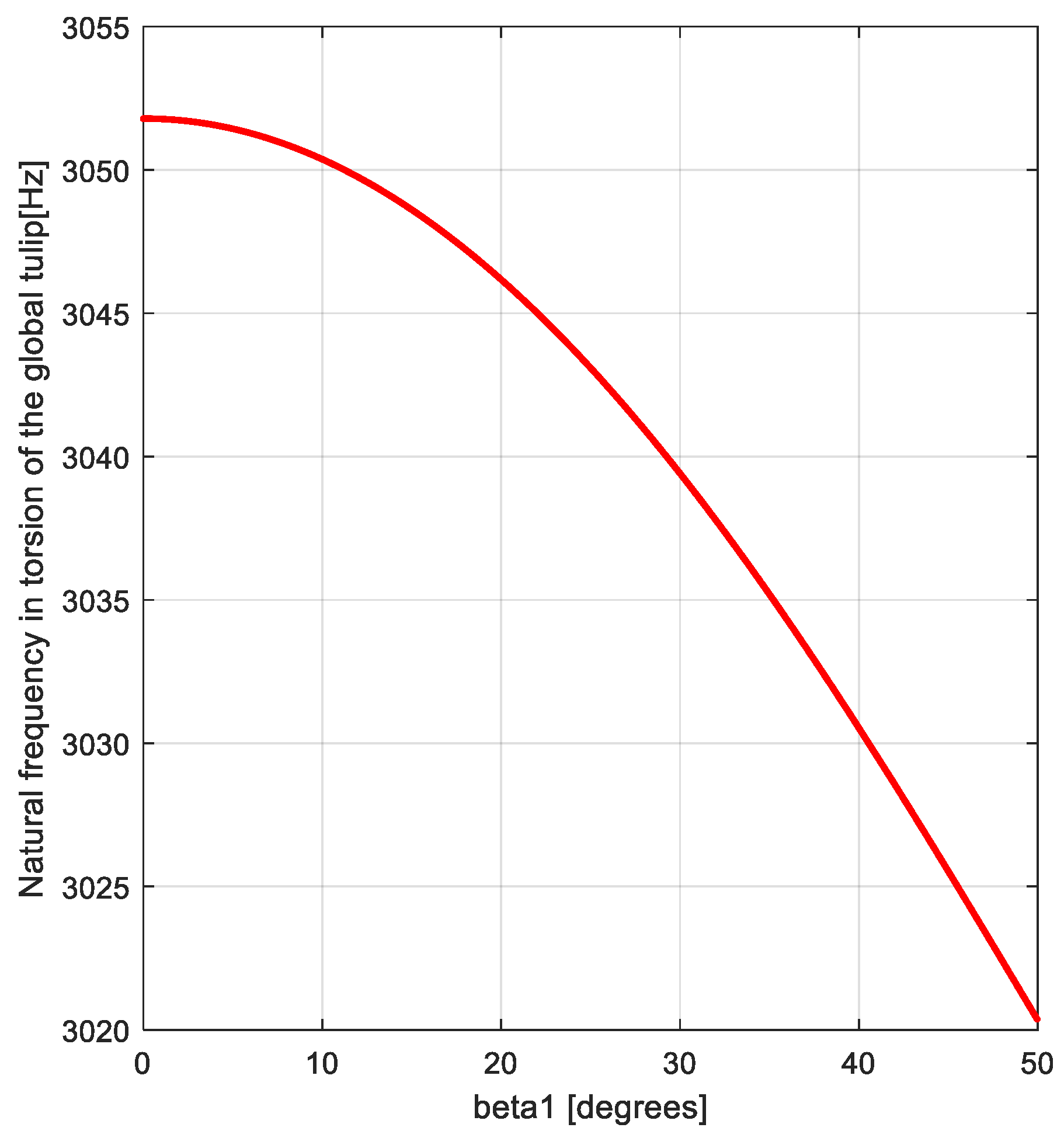
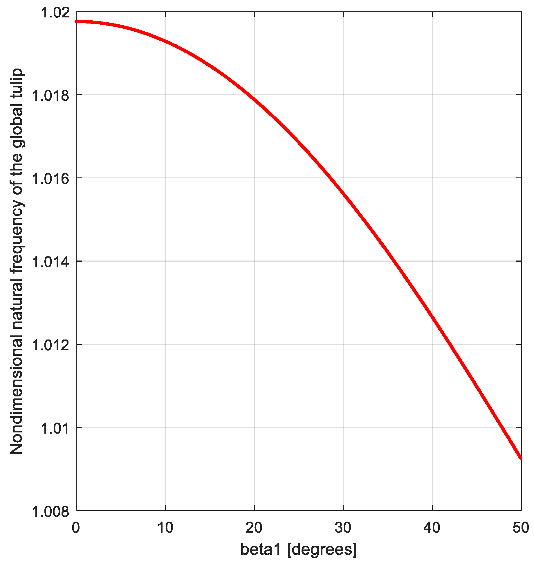
Using the data presented in Table 1 and Table 2 in Equation (41), the variation in ${\overline{\Omega }}_1$, the natural frequency in torsion of the global tulip, was computed as a function of the angle ${\mathsf{\beta }}_1$ using MATLAB software. The data are presented in Figure 7 and Figure 8.

Comparing these theoretical results with those presented in the literature [5] (pp. 119, 125, 138, 139), it can be concluded that there is agreement of the model with the experimental data. To compute the amplitude of the forced torsional nonlinear parametric vibrations in the region of principal parametric resonance, the method of harmonic balance was used [26] (p. 66) for Equation (40) in seeking a solution given by the equation

$$\begin{array}{l}{\mathsf{\phi }}_1(\mathrm{t})=\mathrm{a}\cos \left(\frac{\mathsf{\eta }\mathrm{t}}{2}\right)+\mathrm{b}\sin \left(\frac{\mathsf{\eta }\mathrm{t}}{2}\right),\\ {\Phi }_1=\sqrt{{\mathrm{a}}^2+{\mathrm{b}}^2},\end{array}$$

(45)

where $\mathsf{\eta }\simeq 2{\overline{\Omega }}_1\left(0\right)$ is the excitation frequency and ${\Phi }_1$ is the amplitude of the steady-state vibration in the region of principal parametric resonance for the global tulip. The method is very effective and gives good results, as mentioned in [27], being even now, after half a century, a very convenient method for the analysis of large-scale nonlinear mechanical systems [27]. Before inserting Equation (45) in Equation (40), it is necessary to conduct some mathematical manipulations of Equation (40), such as developing, in Maclaurin series, the following functions around the value 0:

$$\cos 2{\mathsf{\phi }}_1\simeq 1-2{\mathsf{\phi }}_1^2,$$

(46)

$$\sin 3{\mathsf{\phi }}_1\simeq 3{\mathsf{\phi }}_1-4.5{\mathsf{\phi }}_1^3,$$

(47)

$$\sqrt{\frac{1+{\mathrm{a}}_1\cos 2{\mathsf{\phi }}_1}{\left(1+{\mathrm{a}}_2\cos 2{\mathsf{\phi }}_1\right)\left(1+{\mathsf{\chi }}_{\mathrm{G}\mathrm{T}\mathrm{n}}\cos 2{\mathsf{\phi }}_1\right)}}\simeq \sqrt{{\mathrm{A}}_1}+\sqrt{{\mathrm{B}}_1}-\frac{1}{2}\left({\mathrm{a}}_2\sqrt{{\mathrm{A}}_1}+{\mathsf{\chi }}_{\mathrm{G}\mathrm{T}\mathrm{n}}\sqrt{{\mathrm{B}}_1}\right)\left(1-2{\mathsf{\phi }}_1^2\right),$$

(48)

where the terms A₁ and B₁ are expressed in Appendix A. Inserting now the solution given by Equation (45) in Equation (40) and balancing the terms in $\cos \left(\frac{\mathsf{\eta }\mathrm{t}}{2}\right)$ and $\sin \left(\frac{\mathsf{\eta }\mathrm{t}}{2}\right)$ in the unknowns a and b yields the system of equations

$$\{\begin{array}{l}\mathrm{a}\left[\frac{{\mathrm{A}}_1}{1+{\mathrm{a}}_2\mathrm{y}}+\frac{{\mathrm{B}}_1+\mathsf{\gamma }}{1+{\mathsf{\chi }}_{\mathrm{G}\mathrm{T}\mathrm{n}}\mathrm{y}}-\frac{\mathsf{\eta }}{2{\overline{\Omega }}_1}\right]+\mathrm{b}\left[{\mathsf{\alpha }}_1-{\mathsf{\alpha }}_2\mathrm{y}\right]\left[\frac{\mathsf{\eta }}{2{\overline{\Omega }}_1}\right]=0,\\ \mathrm{a}\left[-{\mathsf{\alpha }}_1+{\mathsf{\alpha }}_2\mathrm{y}\right]\left[\frac{\mathsf{\eta }}{2{\overline{\Omega }}_1}\right]+\mathrm{b}\left[\frac{{\mathrm{A}}_1}{1+{\mathrm{a}}_2\mathrm{y}}+\frac{{\mathrm{B}}_1+\mathsf{\gamma }}{1+{\mathsf{\chi }}_{\mathrm{G}\mathrm{T}\mathrm{n}}\mathrm{y}}-\frac{\mathsf{\eta }}{2{\overline{\Omega }}_1}\right]=0,\end{array}$$

(49)

where y is a changing variable of the unknown amplitude ${\Phi }_1$ expressed by the relation

$$\mathrm{y}=1-2{\Phi }_1^2,$$

(50)

where the term $\mathsf{\gamma }$ is the participation of the engine excitation given by the equation

$$\mathsf{\gamma }=\frac{{\overline{\mathrm{M}}}_{\mathrm{e}}}{{\overline{\mathrm{I}}}_{{\mathrm{X}}_2\mathrm{G}\mathrm{T}}},$$

(51)

and the terms α₁ and ${\mathsf{\alpha }}_2$ are presented in Appendix A, while the terms of higher order are neglected in the first order approximation [25] (pp. 425–426), [26] (pp. 63–68). Ensuring a nontrivial solution of the system of Equation (49) yields the following equation, given by setting the determinant of the system (49) to zero:

$${\left[\frac{{\mathrm{A}}_1}{1+{\mathrm{a}}_2\mathrm{y}}+\frac{{\mathrm{B}}_1+\mathsf{\gamma }}{1+{\mathsf{\chi }}_{\mathrm{G}\mathrm{T}\mathrm{n}}\mathrm{y}}-\frac{\mathsf{\eta }}{2{\overline{\Omega }}_1}\right]}^2+{\left[{\mathsf{\alpha }}_1-{\mathsf{\alpha }}_2\mathrm{y}\right]}^2{\left[\frac{\mathsf{\eta }}{2{\overline{\Omega }}_1}\right]}^2=0.$$

(52)

Equation (52) can be transformed into a bi-sextic algebraic equation in the unknown y

$${\Gamma }_1{\overline{\mathsf{\eta }}}^2{\mathrm{y}}^6+{\Gamma }_2{\overline{\mathsf{\eta }}}^2{\mathrm{y}}^5+{\Gamma }_3{\overline{\mathsf{\eta }}}^2{\mathrm{y}}^4+\left[{\Gamma }_4{\overline{\mathsf{\eta }}}^2+{\Gamma }_5\overline{\mathsf{\eta }}\right]{\mathrm{y}}^3+\left[{\Gamma }_6{\overline{\mathsf{\eta }}}^2+{\Gamma }_7\overline{\mathsf{\eta }}+{\Gamma }_8\right]{\mathrm{y}}^2+\left[{\Gamma }_9{\overline{\mathsf{\eta }}}^2+{\Gamma }_{10}\overline{\mathsf{\eta }}+{\Gamma }_{11}\right]\mathrm{y}+{\Gamma }_{12}{\overline{\mathsf{\eta }}}^2+{\Gamma }_{13}\overline{\mathsf{\eta }}+{\Gamma }_{14}=0,$$

(53)

where $\overline{\mathsf{\eta }}=\frac{\mathsf{\eta }}{2{\overline{\Omega }}_1}$ is the nondimensional excitation frequency in the region of principal parametric resonance and the terms ${\Gamma }_1$ to ${\Gamma }_{14}$ are presented in Appendix A. The amplitude of the forced torsional nonlinear parametric vibrations in the region of principal parametric resonance for the global tulip, as a function of nondimensional excitation frequency, is given by the equation

$${\Phi }_1\left(\overline{\mathsf{\eta }}\right)=\sqrt{\frac{1-{\mathrm{y}}^{•}}{2}},$$

(54)

where ${\mathrm{y}}^{•}$ represent the solution of Equation (53). Equations (53) and (54) were used together with all the terms expressed in Appendix A to developed MATLAB software for computing the amplitude of the forced torsional nonlinear parametric vibrations in the region of principal parametric resonance for the global tulip for the steady-state torsional vibrations of the automotive driveshaft. In the same mathematical manner, the amplitude ${\Phi }_3$ of the forced torsional nonlinear parametric vibrations for the global bowl can be computed as a function of nondimensional excitation frequency $\overline{\mathsf{\eta }}=\frac{\mathsf{\eta }}{2{\overline{\Omega }}_3}$ in the region of principal parametric resonance $\mathsf{\eta }\approx 2{\overline{\Omega }}_3$ for the steady-state torsional vibrations of the automotive driveshaft.

7. Results and Discussions

The first results obtained are represented by the natural frequency in torsion of the midshaft given by the modified Equation (36).

$${\mathsf{\nu }}_{\mathrm{n}}=\frac{{\mathsf{\omega }}_{\mathrm{n}}}{2\mathsf{\pi }}=\frac{\mathrm{n}}{2{\mathrm{L}}_{\mathrm{M}\mathrm{s}}}\sqrt{\frac{\mathrm{G}}{\mathsf{\rho }}},\mathrm{n}=1,2,3,\dots$$

(55)

Using this equation, the first three-order natural frequencies for the given midshaft are presented in

Table 3. The first three-order natural frequencies in torsion of the midshaft.

Order	1	2	3
${\mathsf{\nu }}_{\mathrm{n}}$ [Hz]	3338.31	6676.63	10,014.94

(see Table 1 for L_Ms and Table 2 for G and $\mathsf{\rho }$).

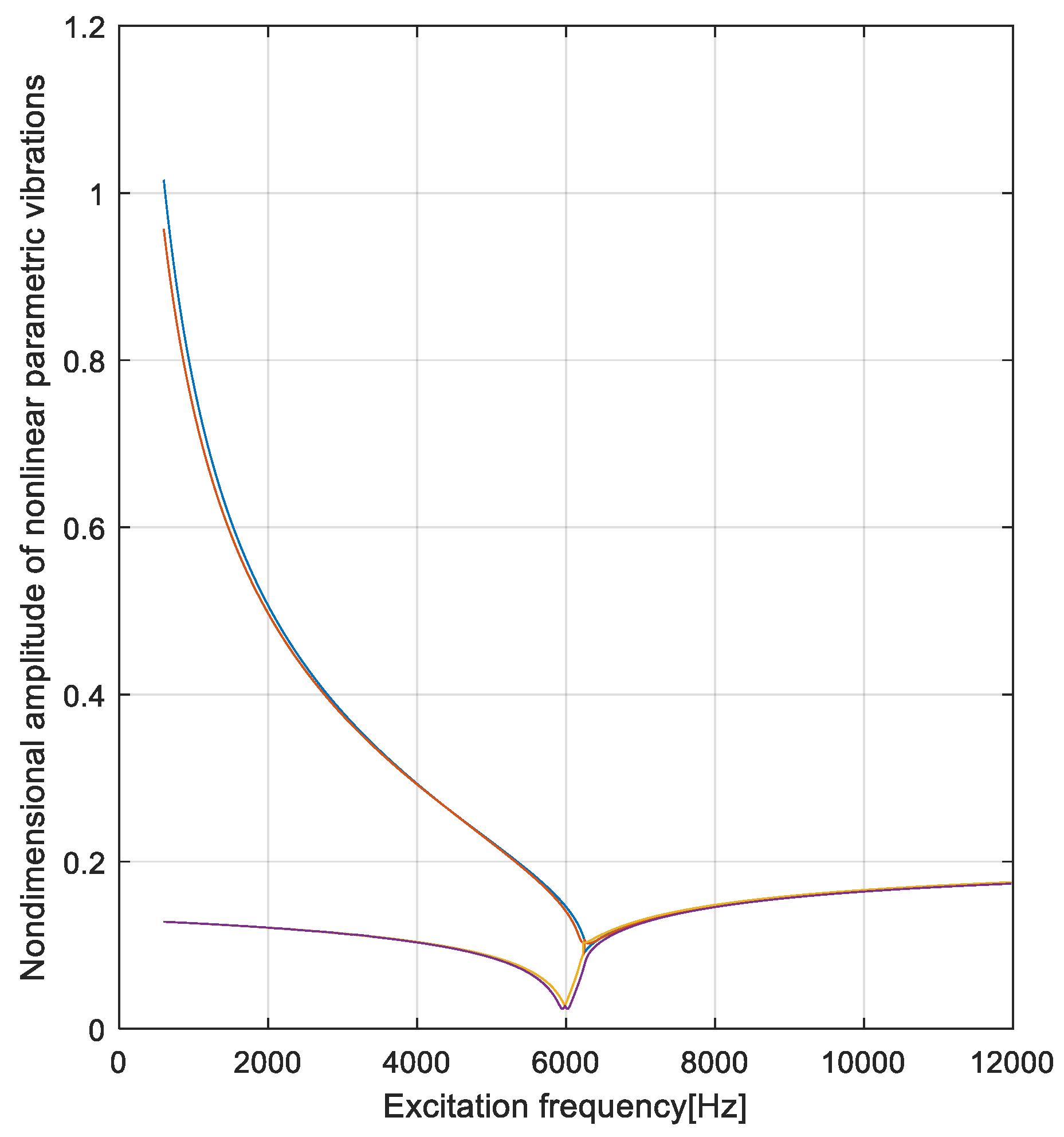
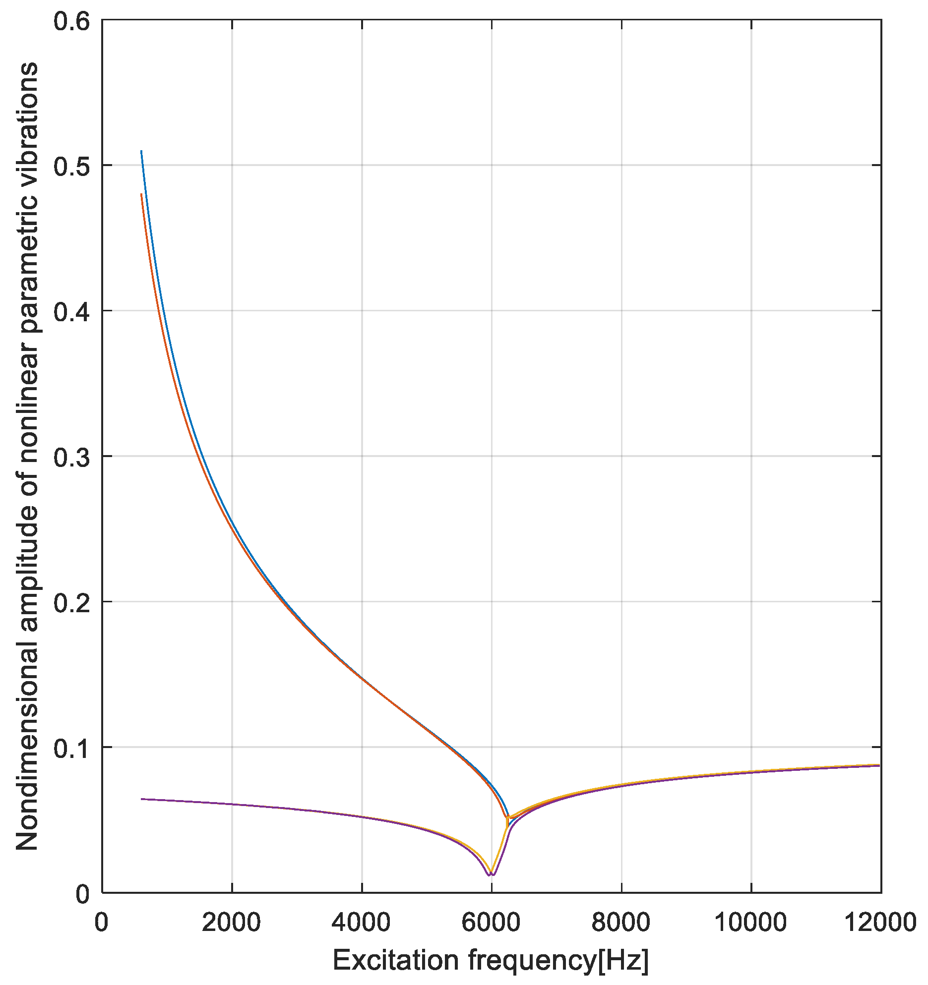
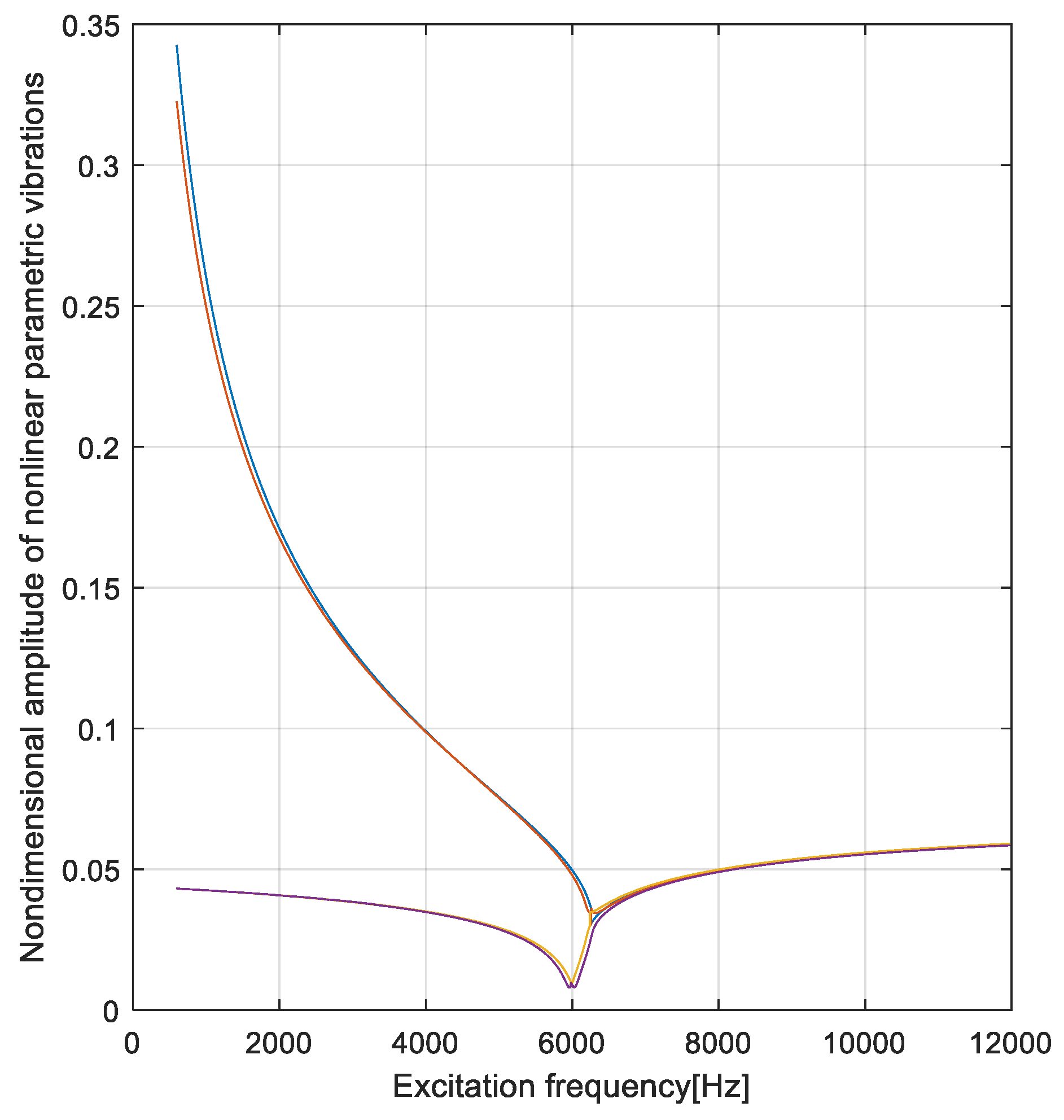
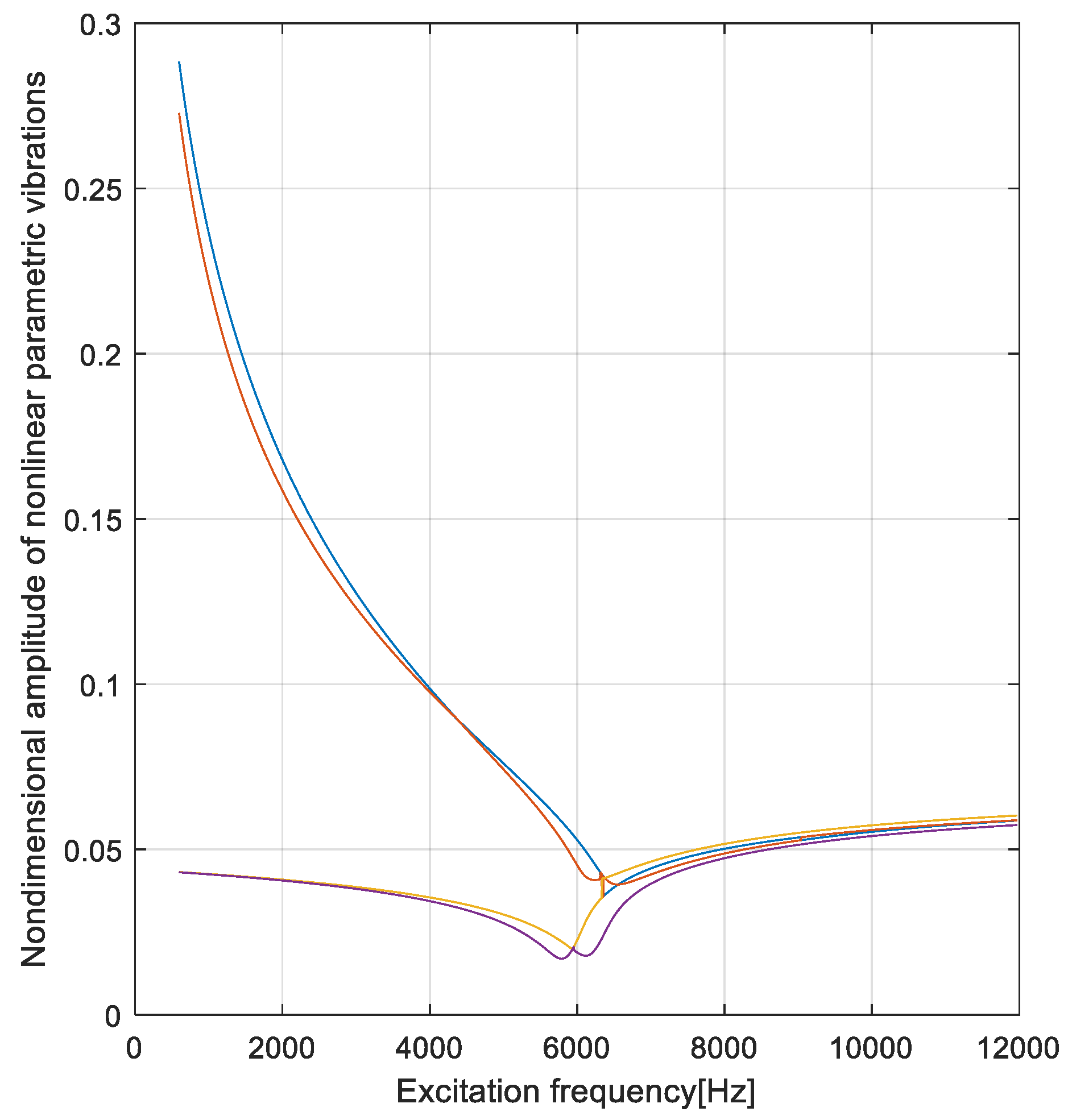
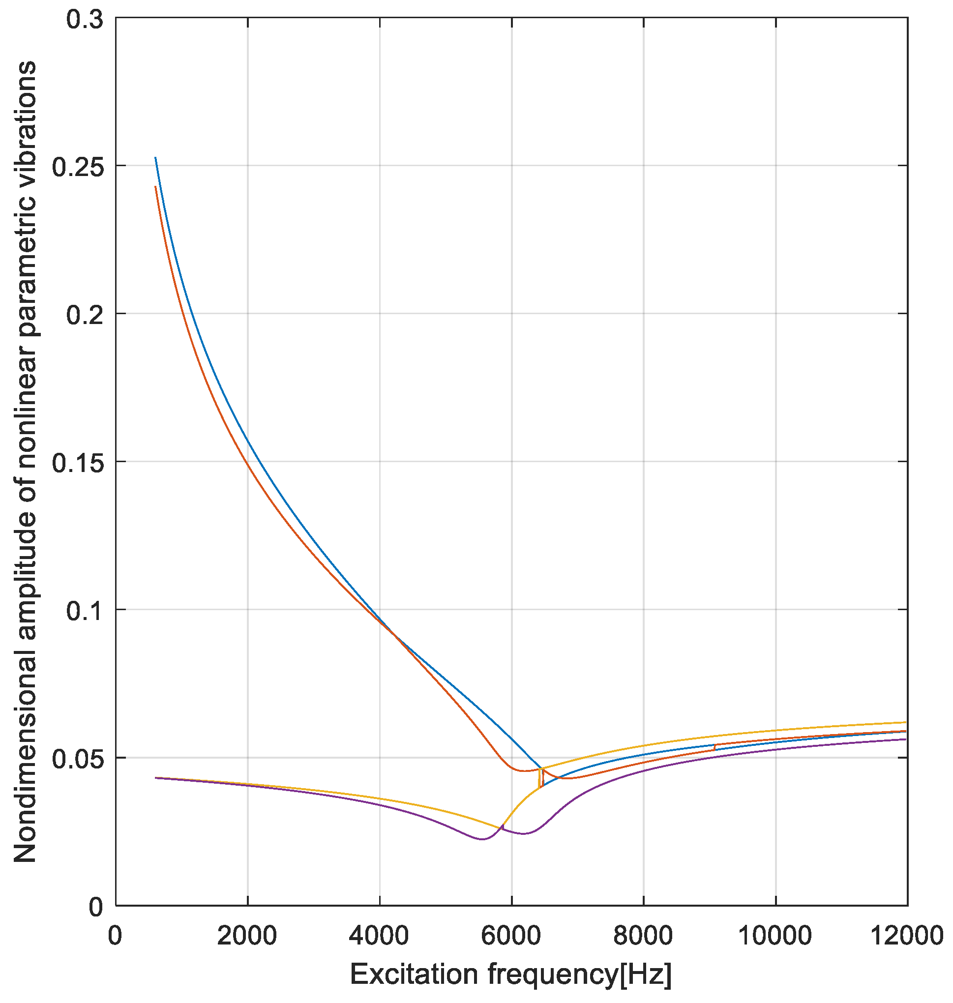
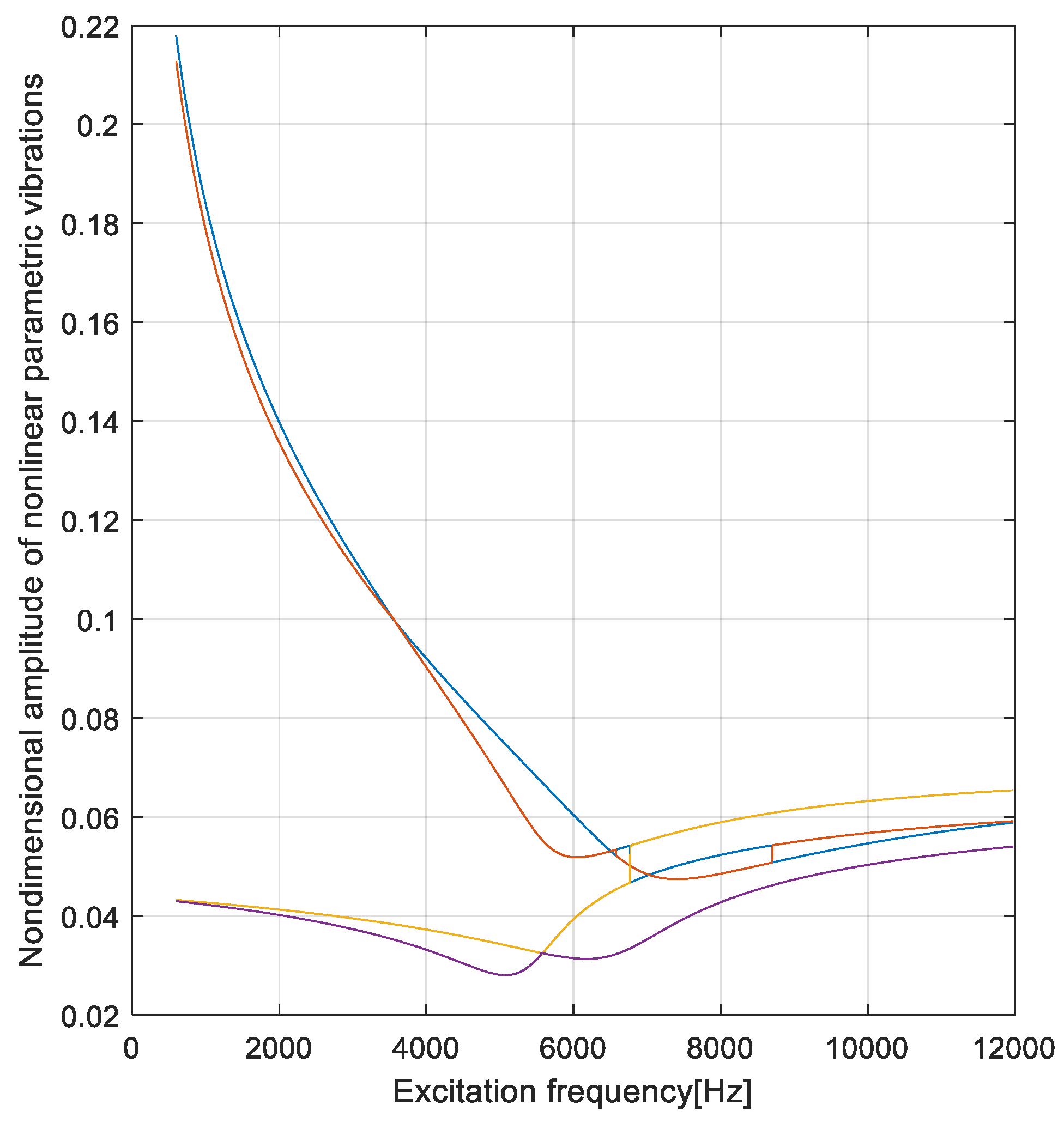
Equation (55) undoubtedly conforms with the experimental data [23] (p. 281). This is also in accordance with the experiments of Steinwede that impose an investigation of the forced torsional vibration of a driveshaft in the range 1–15 kHz [5] (p. 119). The other studies in the literature found, through experiments, that the range of natural free frequencies in the driveshaft torsion [18] in the range 131–906 Hz are, in effect, subharmonic frequencies, that result in misunderstanding of the dynamic phenomena of the automotive driveshaft. From the analyses in Figure 7 and Figure 8, the variation in the natural frequency in torsion of the global tulip is restricted to natural frequency in torsion of the midshaft being in the range 3020–3052 Hz (see Figure 7), and the nondimensional natural frequency in torsion of the global tulip is in the range 1.009–1.0198. Unfortunately, there are no published experiments that investigate the natural free frequency in torsion only for the global tulip. In Figure 9, Figure 10, Figure 11, Figure 12, Figure 13 and Figure 14 is presented the variation of the nondimensional amplitude for forced torsional nonlinear parametric vibration in the region of principal parametric resonance for the global tulip, this being around 5.985 kHz. The nondimensional amplitude presented in the graphs in Figure 9, Figure 10, Figure 11, Figure 12, Figure 13 and Figure 14 represents the normalized amplitude with respect to its maximum value for β₁ = 5°, ζ₁ = 0.0016, ${\mathsf{\chi }}_{\mathrm{n}\mathrm{T}}$ = 0.15. Analyzing Figure 9, Figure 10, Figure 11, Figure 12, Figure 13 and Figure 14, it can be remarked that for the cases we have a manifestation of “soft spring” with two branches for $\mathsf{\eta }\le 1.8{\overline{\Omega }}_1(0)$ that indicate the presence of interaction between principal parametric resonance and the primary resonance, while for $\mathsf{\eta }\ge 1.8{\overline{\Omega }}_1(0)$, only one “hard spring” branch exists, which indicates the manifestation of pure principal parametric resonance for the global tulip [28] (pp. 132–160). The aspect highlighted by Figure 9, Figure 10 and Figure 11 is that with the increase in the angle β₁, the maximum value of the nondimensional amplitude decreases from 1 to 0.35. This aspect agrees with the experimental data in the literature [5] (pp. 130–144). Figure 11, Figure 12, Figure 13 and Figure 14 indicate that, for an angle β₁ = 15° = const., the increase in the damping ratio ζ₁ in the range 0.008–0.0318 induces a decrease in the maximum nondimensional amplitude from 0.35 to 0.22, and, thus, we can conclude that the model is much more sensitive to the geometric variation in the driveshaft than to the damping effects. Through experiments, Steinwede demonstrated that the nonlinear parametric dynamic behavior of automotive driveshafts is like that of geared systems [5] (p. 117), and this is why we observe similar pitting phenomena inside the tulip and inside the bowl of the CVJ joints’ tulip–tripod and bowl–balls–inner race [5] (pp. 88–94). Moreover, it can be seen from Figure 11, Figure 12, Figure 13 and Figure 14 that the increase in damping ratio ζ₁ in the range 0.008–0.0318 induces an increase between the branches of the amplitude for both areas of “soft spring” and “hard spring”, being a manifestation of the multiple “jumps” between the amplitude branches, where it is known that the inferior branch is usually unstable, while the superior branch is stable [25] (pp. 426–429), [28] (pp. 132–160). This aspect will “conduct” dynamic behavior through a chaotic dynamic that has, as a practical effect, an accelerating effect on pitting phenomena, as mentioned by Steinwede [5] (pp. 88–94), or in the worst case, results in the manifestation of cracks followed by failure (breaking) of the global tulip [5] (p. 89). Unfortunately, there are no published studies analyzing, in detail, the dynamic behavior of each element of the automotive CVJ driveshaft: tulip, global tulip, bowl, global bowl, and midshaft, apart from [5], where all studies have analyzed the global dynamic behavior of the automotive driveshaft. Even so, there is huge confusion regarding the interpretation of experimental data due to the misunderstanding of specific global nonlinear phenomena, such as in [18].

Based on the aspects presented above, the direction for future research involves the investigation of analytical solutions of the system of Equations (40) and (43) using the multiple scale method for each type of resonance, as mentioned before. Another future research direction is to investigate stability in the proximity of each possible resonance type for steady state as well as nonstationary motion.

8. Conclusions

The present work introduces a complex model for torsional vibrations of the automotive driveshaft, a model that considers most of the phenomena observed in industrial practice and the exploitation of cars such as:

-

nonuniformity in the geometric and kinematic isometry of the driveshaft;

-

nonuniformity in the geometric and mass moments of inertia of the cross section for the tulip, tripod, inner race, and bowl;

-

the stiffness and the damping link of the joints of the driveshaft tulip–tripod–midshaft and midshaft–inner race–balls–bowl;

-

harmonic excitation of the driveshaft due to the car engine;

-

impulsive excitation of the driveshaft due to road excitation.

In addition, the model allows the development of future research directions for the investigation of primary resonances, super harmonic resonances, subharmonic resonances, principal parametric resonances, combination resonances, internal resonances, and simultaneous resonances as well as for investigation of the stability for steady-state as well as nonstationary motion. Therefore, this model of dynamic torsional behavior for the automotive driveshaft can be used in the early stages of design as well in predicting the durability of automotive driveshafts. Moreover, it is important that the model be added in the design algorithm for predicting the comfort elements of motoring to adequately account for this kind of dynamic behavior, which induces excitations to the car structure as mentioned in the literature [15].

References

- Duditza, F.; Diaconescu, D. Zur Kinematik und Dynamik von Tripode-Gelenkgetrieben. Konstruction 1975, 27, 335–341. [Google Scholar]
- Grünwald, B. Theory, Computation and Design of Internal Combustion Engines for Automotive; Didactic &Pedagogical Publishing House: Bucharest, Romania, 1980. (In Romanian) [Google Scholar]
- Sireteanu, T.; Gündisch, O.; Paraian, S. Random Vibrations of Automotive; Technical Publishing House: Bucharest, Romania, 1981. (In Romanian) [Google Scholar]
- Bugaru, M.; Vasile, A. Nonuniformity of Isometric Properties of Automotive Driveshafts. Computation 2021, 9, 145. [Google Scholar] [CrossRef]
- Steinwede, J. Design of a Homokinetic Joint for Use in Bent Axis Axial Piston Motors. Ph.D. Thesis, PhD-Granting by Aachen University, Aachen, Germany, 25 November 2020. Available online: https://www.google.com/search?client=firefox-b-d&q=%E2%80%9DDESIGN+OF+A+HOMOKINETIC+JOINT+FOR+USE+IN+BENT+AXIS+AXIAL+PISTON+MOTORS%E2%80%9D+J.+Steinwede+ (accessed on 19 December 2021).
- Mazzei, A.J.; Scott, R.A. Principal Parametric Resonance Zones of a Rotating Rigid Shaft Driven through a Universal Joint. J. Sound Vib. 2001, 244, 555–562. [Google Scholar] [CrossRef] [Green Version]
- Browne, M.; Palazzolo, A. Super harmonic nonlinear lateral vibrations of a segmented driveline incorporating a tuned damper excited by a non-constant velocity joints. J. Sound Vib. 2008, 323, 334–351. [Google Scholar] [CrossRef] [Green Version]
- Feng, H.; Rakheja, S.; Shangguan, W.B. Analysis and optimization for generated axial force of a driveshaft system with interval of uncertainty. Struct. Multidiscip. Optim. 2021, 63, 197–210. [Google Scholar] [CrossRef]
- Tiberiu-Petrescu, F.I.T.; Petrescu, R.V.V. The structure, geometry, and kinematics of a universal joint. Indep. J. Man Agement Prod. 2019, 10, 1713–1724. [Google Scholar] [CrossRef]
- Ertürka, A.T.; Karabayb, S.; Baynalc, K.; Korkutd, T. Vibration Noise Harshness of a Light Truck Driveshaft, Analysis and Improvement with Six Sigma Approach. Acta Phys. Pol. A 2017, 131, 477–480. [Google Scholar] [CrossRef]
- Kamalakkannan, B. Modelling and Simulation of Vehicle Kinematics and Dynamics. Master’s Thesis, Master-Granting by Halmstad University, Hogskolan i Halmstad, Sweden, 13 January 2017. [Google Scholar]
- Kishore, M.; Keerthi, J.; Kumar, V. Design and Analysis of Drive Shaft of an Automobile. Int. J. Eng. Trends Technol. 2016, 38, 291–296. [Google Scholar] [CrossRef]
- Shao, K.; Zheng, J.; Huang, K.; Qiu, M.; Sun, Z. Robust model referenced control for vehicle rollover prevention with time-varying speed. Int. J. Veh. Des. 2021, 85, 48–68. [Google Scholar] [CrossRef]
- Deng, B.; Zhao, H.; Shao, K.; Li, W.; Yin, A. Hierarchical Synchronization Control Strategy of Active Rear Axle Independent Steering System. Appl. Sci. 2020, 10, 3537. [Google Scholar] [CrossRef]
- Farshidianfar, A.; Ebrahimi, M.; Rahnejat, H.; Menday, M.T.; Moavenian, M. Optimization of the high-frequency torsional vibration of vehicle driveline systems using genetic algorithms. Proc. Inst. Mech. Eng. Part K J. Multi-Body Dyn. 2002, 216, 249–262. [Google Scholar] [CrossRef] [Green Version]
- Komorska, I.; Puchalski, A. On-board diagnostics of mechanical defects of the vehicle drive system based on the vibration signal reference model. J. Vibroeng. 2013, 15, 450–458. Available online: https://www.jvejournals.com/article/14460 (accessed on 19 December 2021).
- Alugongo, A.A. Parametric Vibration of a Cardan Shaft and Sensitivity Analysis. In Proceedings of the World Congress on Engineering and Computer Science 2018 Vol II WCECS, San Francisco, CA, USA, 23–25 October 2018; Available online: https://www.google.com/search?client=firefox-b-d&q=Parametric+Vibration+of+a+Cardan+Shaft+and+Sensitivity+Analysis+Alfayo+A.+Alugong (accessed on 19 December 2021).
- Xu, J.; Zhu, J.; Xia, F. Modeling and Analysis of Amplitude-Frequency Characteristics of Torsional Vibration for Automotive Powertrain. Hindawi Shock Vib. 2020, 2020. [Google Scholar] [CrossRef]
- Idehara, S.J.; Flach, F.L.; Lemes, D. Modeling of nonlinear torsional vibration of automotive powertrain. J. Vib. Control. 2018, 24, 1774–1786. [Google Scholar] [CrossRef]
- Bugaru, M.; Chereches, T.; Trana, E.; Gheorghian, S.; Homotescu, T.N. Theoretical model of the dynamic interaction between wagon train and continuous rail. WSEAS Trans. Math. 2006, 5, 374–378. Available online: https://0-scholar-google-com.brum.beds.ac.uk/citations?view_op=view_citation&hl=en&user=tYI6MzwAAAAJ&citation_for_view=tYI6MzwAAAAJ:_FxGoFyzp5QC (accessed on 19 December 2021).
- Deciu, E.; Bugaru, M.; Dragomirescu, C. Nonlinear Vibrations with Applications in Mechanical Engineering; Romanian Academy Publishing House: Bucharest, Romania, 2002; ISBN 973-27-0911-1. [Google Scholar]
- Seherr-Thoss, H.C.; Schmelz, F.; Aucktor, E. Designing Joints and Driveshafts. In Universal Joints and Driveshafts, 2nd ed.; Springer: Berlin/Heidelberg, Germany, 2006; pp. 109–248. [Google Scholar]
- Rao, S.S. Torsional Vibrations of Shafts. In Vibration of Continuous Systems; John Wiley & Sons: Hoboken, NJ, USA, 2007; pp. 272–316. ISBN 978-0-471-77171-5. [Google Scholar]
- Rao, S.S. Mechanical Vibrations, 5th ed.; Prentice Hall: Upper Saddle River, NJ, USA, 2011; ISBN 978-0-13-212819-3. [Google Scholar]
- Nayfeh, A.H.; Mook, D.T. Nonlinear Oscillations; John Wiley & Sons: Hoboken, NJ, USA, 1979. [Google Scholar]
- Bolotin, V.V. Dynamic Stability of Elastic Systems, 2nd ed.; US Military Report; Aerospace Corporation: El Segundo, CA, USA, 1962. [Google Scholar]
- Detroux, T.; Renson, L.; Masset, L.; Kerschen, G. The harmonic balance method for bifurcation analysis of large-scale nonlinear mechanical systems. Comput. Methods Appl. Mech. Eng. 2015, 296, 18–38. [Google Scholar] [CrossRef] [Green Version]
- Bugaru, M. Dynamic Behavior of Geared System Transmission. Ph.D. Thesis, PhD-Granting by Auburn University & University Politehnica of Bucharest (Joint Ph.D. Program Romania-University POLITEHNICA of Bucharest/USA-Auburn University/Germany-Technische Universitat Munich Based on Deuche Forschung Gemeinschaft-VDI), Auburn, AL, USA, Bucharest, Romania, 13 October 2004. Available online: https://crescdi.pub.ro/#/profile/804 (accessed on 17 December 2021).
Figure 1.
An automotive driveshaft.
Figure 2.
Driveshaft in general detail.
Figure 3.
Schematic representation of an automotive driveshaft.
Figure 4.
Details of tulip–tripod (tripod of the midshaft) joint.
Figure 5.
Details of bowl–balls (inner race of the midshaft) joint.