
Computational Analysis of Active and Passive Flow Control for Backward Facing Step


Laboratory of Biofluid Mechanics & Biomedical Engineering, School of Mechanical Engineering, National Technical University of Athens, Zografos, 15780 Athens, Greece
*
Author to whom correspondence should be addressed.
Computation 2022, 10(1), 12; https://0-doi-org.brum.beds.ac.uk/10.3390/computation10010012
Submission received: 18 November 2021
/
Revised: 7 January 2022
/
Accepted: 13 January 2022
/
Published: 16 January 2022
(This article belongs to the Special Issue Experiments/Process/System Modeling/Simulation/Optimization (IC-EPSMSO 2021))
Abstract
:The internal steady and unsteady flows with a frequency and amplitude are examined through a backward facing step (expansion ratio 2), for low Reynolds numbers (, ), using the immersed boundary method. A lower part of the backward facing step is oscillating with the same frequency as the unsteady flow. The effect of the frequency, the amplitude, and the length of this oscillation is investigated. By suitable active control regulation, the recirculation lengths are reduced, and, for a percentage of the time period, no upper wall, negative velocity, region occurs. Moreover, substituting the prescriptively moving surface by a pressure responsive homogeneous membrane, the fluid–structure interaction is examined. We show that, by selecting proper values for the membrane parameters, such as membrane tension and applied external pressure, the upper wall flow separation bubble vanishes, while the lower one diminishes significantly in both the steady and the unsteady cases. Furthermore, for the time varying case, the length fluctuation of the lower wall reversed flow region is fairly contracted. The findings of the study have applications at the control of confined and external flows where separation occurs.
1. Introduction
Flow separation arises innately in internal and external flows, incurring losses. The suppression of the effects of the detached flow, such as pressure drop or drag, is a common goal of fluid dynamics analysis and design. The inner flow past a backward facing step (BFS) constitutes a benchmark problem for the analysis of recirculation owing to its simplicity, along with the fixation of the lower wall detachment position at the step location [1,2]. Backward facing step flow applications abound in everyday life. Bubble zones at the wake of vehicles, separated flow over airfoils at large attack angles, spoiler flows, detachment of inflow in an engine, and bubble downstream flows around constructions/ships are common cases of backward facing step flow applications occuring in modern practices [3]. For the control of the flow, various methods have been applied, such as plasma actuation, electromagnetic actuation, synthetic jet, oscillating flap, inlet pulsation, periodic perturbation, vortex generators, local forcing, and visual feedback [3,4,5,6,7,8,9,10,11] etc.
The oscillating flow past a BFS having the same frequency as the moving portion of the bottom wall is simulated by Mateescu and Venditti [12] and Mateescu et al. [13]. Under several values of the periodical inflow amplitude, the positions where detachment or reattachment occurs are calculated for various surface oscillation amplitude and frequency values for a range of low and intermediate inflow Reynolds numbers (400–1000). The Navier–Stokes equations are discretized with a second order backward implicit scheme and an artificial compressibility scheme is employed for the coupling of the equations. The pseudotime discretization is performed using a first order implicit scheme. It is concluded that for increasing wall oscillation amplitude, the upper wall bubble length increases and its presence percentage during the period decreases. They also find that the lower wall bubble length fluctuation increases. For higher Reynolds number values, the length of the separation regions increase significantly, a secondary lower wall separation region emerges and the upper wall separation region is present the whole period. By increasing the oscillation frequency, the fluctuation amplitude of the lower wall closed streamlines length increases, while the upper wall bubble remains nearly unchanged.
Fluid structure interaction (FSI) involving elastic membranes [14] has been extensively studied in biomedical cases and other settings [15,16,17,18]. The steady flow in a 2D channel with one rigid plate, and another with a part of it replaced by an elastic membrane, is perturbed and the resulting flow is studied by Luo and Pedley [19]. It is shown that the steady solutions become unstable as membrane tension falls below a threshold value and self-excited oscillations emerge. The interaction of Poiseuille flow with a tensioned membrane portion of one of the walls with structural damping, is addressed by Huang [20]. The oscillation of the membrane is found to strongly depend on inlet and outlet boundary conditions.
The immersed boundary method [21] has been applied for the computation of the flow over a BFS by Saleel et al. for low Reynolds numbers (0.0001–100) [22]. The authors implement the momentum forcing and the mass source/sink to satisfy, at the solid boundaries, zero flow velocity relative to the boundaries. They employ a finite volume method on a staggered grid with a fractional step in time. Yang et al. apply an LES-immersed boundary approach for the flow over a backward facing step for Reynolds numbers in the turbulent region (5100) [23]. Agreement is found between the results from the IB method coupled with LES and those from DNS and experiments.
The curvilinear immersed boundary method of Ge and Sotiropoulos has been applied for the computation of unsteady incompressible flows [24], such as that in a 2D driven cavity, an impulsively started flow at a square cross-section duct, the pulsatile flow at a circular-section pipe bend and the pulsatile flow in a bileaflet mechanical heart valve (BMHV). Moreover, it has been applied by Borazjani et al. [25] for the research on FSI pertaining to rigid bodies, such as an elastic mounted cylinder in the free stream and the blood flow through a BMHV. Gilmanov et al. [26] extended the method and simulated FSI with thin flexible shells.
In this work, the immersed boundary method [27], in the form proposed by Ge and Sotiropoulos [24], is employed to simulate the control of the confined, viscous, steady, and unsteady, incompressible flow over a backward facing step. The proposed control methods and the findings of the present study for the separation of the flow at the standard case of the flow over a backward facing step, can have a plethora of applications to external and internal industrial and biomedical applications. The momentum equations are integrated in time via a Crank–Nicholson second order implicit scheme. The continuity and momentum equations are coupled via a Poisson equation for pressure correction leading to the satisfaction of the continuity equation. The implementation of the method of Ge and Sotiropoulos [24] for the computation of the fluid structure interaction with a deformable body, where the total fluid volume of the computational domain changes in time, is a novelty aspect of this work.
Initially, the flow characteristics for the BFS under steady and unsteady inflow conditions are presented. Imposing forced oscillatory movement at a portion of its bottom wall, the unsteady flow over the BFS is simulated, examining the effect of the amplitude and the frequency of the oscillating surface. Moreover, the role of the length of the oscillating surface is examined, for which results do not exist in bibliography. Substituting the moving oscillating part of the bottom wall with an elastic membrane, the FSI with the steady and unsteady flow is analyzed. To the best of our knowledge, control of the flow by means of an elastic membrane with direct interaction with the main periodical flow, has not been implemented so far for the BFS. An elastic membrane has the advantage over the rigid passive control means, of adaptability within a range of different inflow conditions, without tuning demanded.
2. Methods
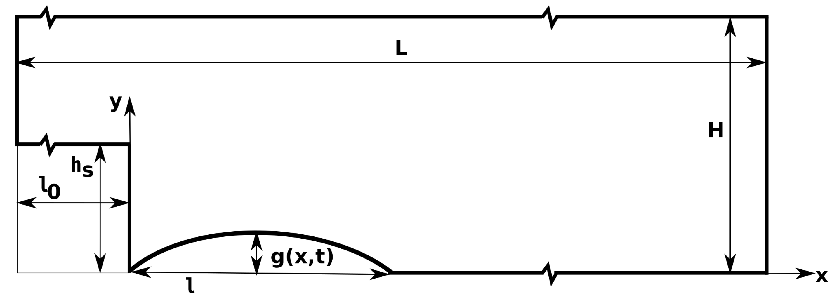
2.1. Geometry and Boundary Conditions of Backward Facing Step with Partly Moving Bottom Wall
A backward facing step with expansion ratio two, i.e., , length upstream of the step and length downstream is examined, following a large part of existing research [28,29,30,31,32].
Dirichlet boundary condition for the velocity in the inlet () is given as [13,30]
where is the inflow velocity oscillation amplitude, u, v are the longitudinal and transverse Cartesian velocity components, respectively, is the angular frequency of the oscillation and t is time. At the outlet () the Neumann boundary conditions
are imposed.
We examine two cases for the function of the position of the moving part of the bottom wall of length l.
- (a)
- Forced motion with frequency the same as the frequency of flow, according to the equation [12]
- (b)
- Fluid–structure interaction between the flow and the moving part of the bottom wall which is considered an elastic membrane. The structure responds to the flow according to the equation of a membrane, under the assumptions of small displacement and small inertia
In the above equation, is the constant tension of the membrane (force per width), is the constant pressure implemented on its external side and the pressure applied by the flow at its internal side, b is the membrane thickness and is its density. The equation of motion of the membrane (Equation (4)) is constrained with the boundary conditions of membrane’s both streamwise ends ( and ) being fixed at
At every wall, including the immersed boundary, no slip boundary conditions are imposed
where is the respective velocity component of the wall.
For the derivation of pressure at the immersed boundary, the following Neumann boundary condition which is deduced by the momentum conservation is implemented [33,34]
where is the position vector, is the normal vector to the immersed surface, and is the velocity of the immersed surface.
A three dimensional methodology is used for the implementation of the immersed boundary method (Section 2.2), therefore a small depth d of the uniform flow field in the z direction is considered, specifically . On the third dimension z, slip boundary conditions are applied
where w is the depthwise Cartesian velocity component.
2.2. Computational Method for the Navier–Stokes Equations
Non-dimensionalization of the geometrical and flow quantities is completed with H for the length, for the velocity, for the pressure and for the membrane tension . In the following, the non-dimensional version of the involved variables is considered, keeping the same symbol for each physical quantity, i.e.,
From here onwards we consider the non-dimensional problem and all referenced quantities are normalized.
The non-dimensional Navier–Stokes equations are solved by means of the immersed boundary method [21] as formulated by Ge and Sotiropoulos [24] in three dimensions, on a curvilinear coordinate system . The Jacobian of the transformation from the Cartesian to the curvilinear base is expressed as
In tensor notation, the symbols employed are for the contravariant velocity component, for the Cartesian velocity component, for the Cartesian coordinate, p for the pressure, for the Reynolds number, and for the contravariant base vector
The discretization of the equations is performed with the bottom wall of the BFS considered an immersed boundary, described by a closed surface mesh consisting of triangles [36,37]. For the discretization on the curvilinear mesh, the flow variables (, , , p) are defined at volume centers while the momentum equations are solved at surface centers, using values for the convective and viscous terms interpolated by the cell centers. Thus, the evaluation of the covariant derivatives of the base vectors, i.e., the Christoffel symbols, is avoided, leading to a reduction in computational cost [24]. In the present study, linear interpolation is used for the derivation of the convective and viscous quantities of the momentum equations at the surface centers [38]
where
The background mesh nodes are categorized as solid, immersed boundary, and fluid. Solid nodes are those to the interior of the closed surface triangular mesh; immersed boundary nodes are those which are less than a cell away and at the outer of the triangular mesh; and fluid nodes are the rest, where the flow equations are solved [25]. The velocity values at an immersed boundary node P are linearly interpolated between the velocity of the closest immersed grid cell C on one side and the velocity of the triangle of fluid nodes neighbor to P intersected by the half line starting at C and passing through P on the other [36].
The time integration of the system of equations is performed via a Crank–Nicholson second order scheme of the form [39]
where
The superscript is employed to refer to the velocity field derived from the solution of the momentum equations and before the projection step, while the superscript refers to the last time step at which the flow is already computed.
The pressure field is computed so as for the incompressibility constraint to be satisfied. For this aim a Poisson equation is solved to obtain a pressure correction field
leading to zero divergence of the velocity field at the next time step [40]. The superscript refers to the next time step to which the computation is targeting.
Owing to the linearity of the operator acting on pressure, the following equation arises for the corrections on the pressure field [41]
Consequently, the velocity component at the new time step is derived from the equation
The resulting nonlinear system for the momentum equations is approximately factorized and solved through the Newton–Krylov generalized minimal residual method (GMRES) [38,42,43]. GMRES is also employed for solving the linear system for pressure corrections arising from the discretization of the Poisson’s equation (Equation (18)) on the background mesh [24].
The implementation of the immersed boundary method and the solution of the Navier–Stokes equations are performed with the Virtual Flow Simulator software (VFS) [44].
2.3. Computational Grids and Discretization Steps
A space and time discretization independence study is performed for each case in order for the underlying grids and time steps to be selected. For the steady case with of Section 3.1, the fine mesh used (2019 × 149 grid points) shows a maximum difference of in detachment–reattachment positions results in comparison to the next coarser mesh (2019 × 134 grid points) that was implemented.
The underlying mesh used in Section 3.1 for the case has 2019 points in x direction and 121 points in y direction. Inflation for x partitioning is applied in the region with step size and for y direction partitioning in the region with step size . Additionally, local inflation near the upper and lower walls is employed. For the case a 3025 × 182 dense grid discretizes the computational domain with for and uniform y partitioning with near wall inflation. The fluid calculation grid consists for the case of ≈732,897 nodes and for the case of ≈1,617,486 nodes.
For Section 3.2, Section 3.3, Section 3.4 and Section 3.5, the background grid has 1721 nodes for x discretization. The minimum x interval, is for to . From to , increases geometrically to the value . For the y discretization 149 and 113 nodes are used for the active and passive control cases computations, respectively. In the forced oscillation case, the minimum y interval, is for y in the region from to and increases geometrically in the interval to the value . From to three more grid lines are located. In the membrane case, the interval with y discretization step is . The rest of y discretization, for , is identical to the oscillating surface case. For the 3D fluid computational domain the calculation grid consists of approximately 600,000 nodes. For the immersed boundary surface mesh used for the moving part of the bottom wall in Section 3.2, Section 3.4 and Section 3.5, the streamwise partitioning is performed with step .
The time step used in Section 3.3 and Section 3.4 is , while in Section 3.5, where the motion of the solid boundary is less intensive in comparison with the active control case, the non-dimensional time is sampled every .
2.4. Fluid–Structure Interaction
For the fluid–structure interaction between the fluid flow and the elastic membrane, the equations of flow are loosely coupled with the boundary value problem (BVP) of the membrane motion equation (Equation (4)) in conjunction with the boundary conditions defined by Equation (5).
The BVP is solved by means of the shooting method, i.e., the integration of the differential equation starts at the one boundary, assuming the value of the derivative at the same point. By applying the Newton–Raphson method, the correct value of the derivative on the boundary where the integration starts is found, aiming at the satisfaction of the boundary condition on the boundary where integration concludes (Algorithm 1) [45].
The ordinary differential equation is solved by employing a fifth order Runge–Kutta method with adaptive step size.
| Algorithm 1 BVP solution | ||
| • Initialization parameters: time instance , tolerance , iteration number , initial membrane inclination at step position | ||
| 1: | define | ▷ Error function, depicting divergence from 2nd BV |
| 2: | ▷ Next integration index | |
| 3: | solve initial value problem of Equation (4), and | |
| 4: | if | ▷ If error greater than tolerance |
| 5: | compute | ▷ Derivative of error with respect to inclination at |
| 6: | compute from Newton–Raphson method | ▷ Zero error desired at next step |
| 7: | repeat from 2 | |
| 8: | else | ▷ BVP problem is satisfied |
| 9: | return | ▷ Return BVP solution |
3. Results and Discussion
In this section, the results for the steady and unsteady flows over the backward facing step without and with control are presented and discussed. The separated in both walls, steady flow of Section 3.1 is passively controlled using an elastic membrane and the results are presented in Section 3.2. The forced control of the unsteady separated flow in Section 3.3 by an oscillating portion of the bottom wall is shown in Section 3.4 and the passive control by an elastic membrane of the same flow is shown in Section 3.5.
3.1. Steady Flow
In Table 1, the characteristic recirculation lengths are presented, for the steady case over the BFS, for Reynolds number
where is the kinematic viscosity of the fluid.
The results for the validation of the method are in close agreement with the existing results obtained via body-fitted methods.
For Reynolds number 400 and we find the lower wall reattachment at and no upper wall separation of the flow.
3.2. Control of Steady Flow Using an Elastic Membrane
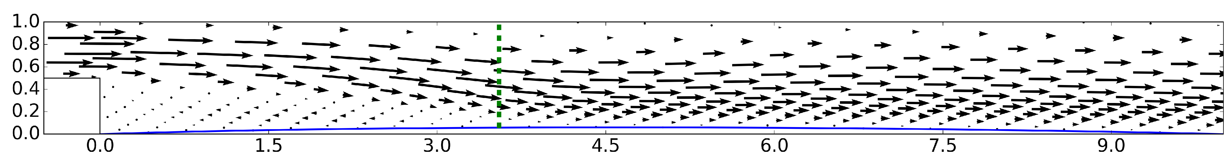
The portion of the rigid bottom wall starting at the step position and having length is substituted with an elastic membrane with tension . The external pressure exerted on the outer surface of the membrane is taken to have the value . The criterion for using this combination of membrane’s parameters is deformation of the membrane to be small and positive and the external pressure to be close to the flow’s pressure. Solving the FSI between the steady flow and the membrane for Reynolds number 400, the velocity vectors are depicted in Figure 2 and Figure 3.
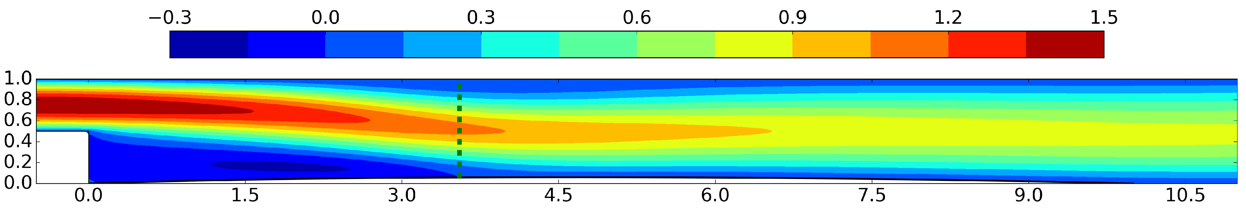
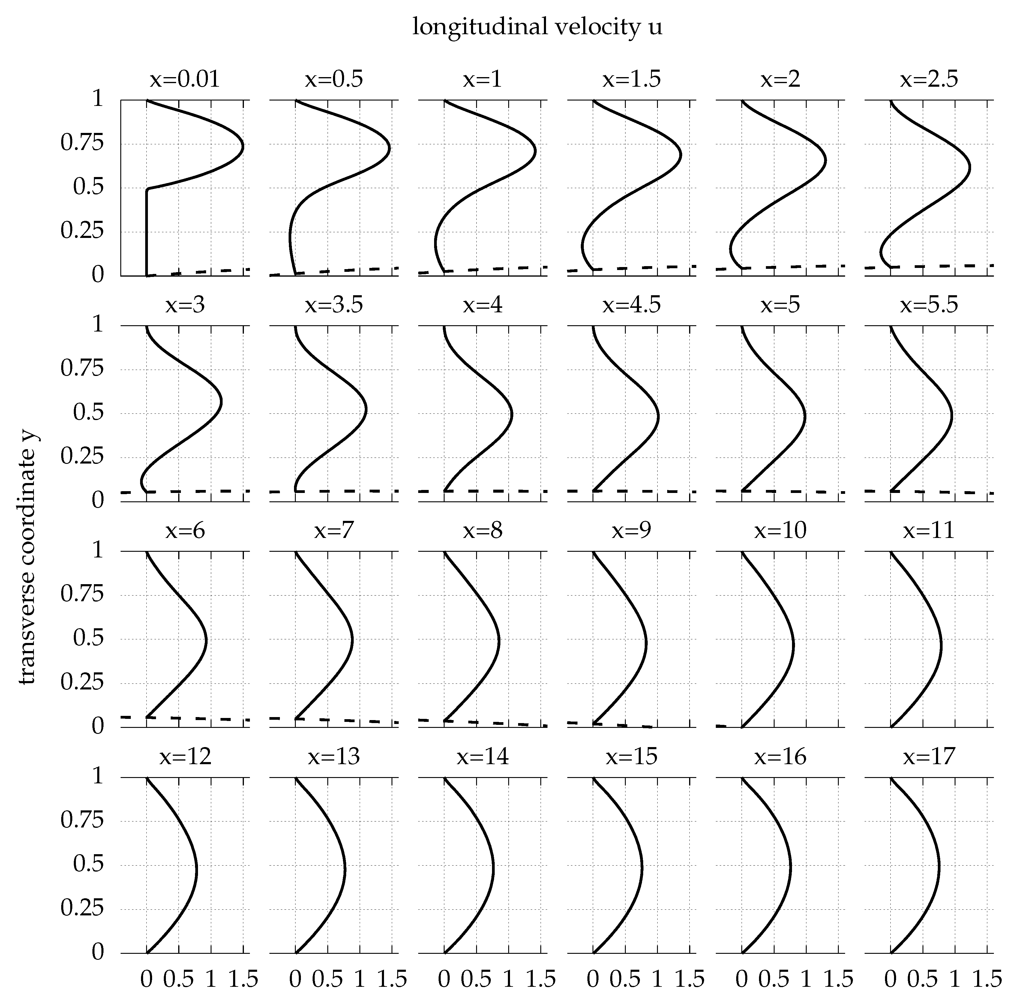
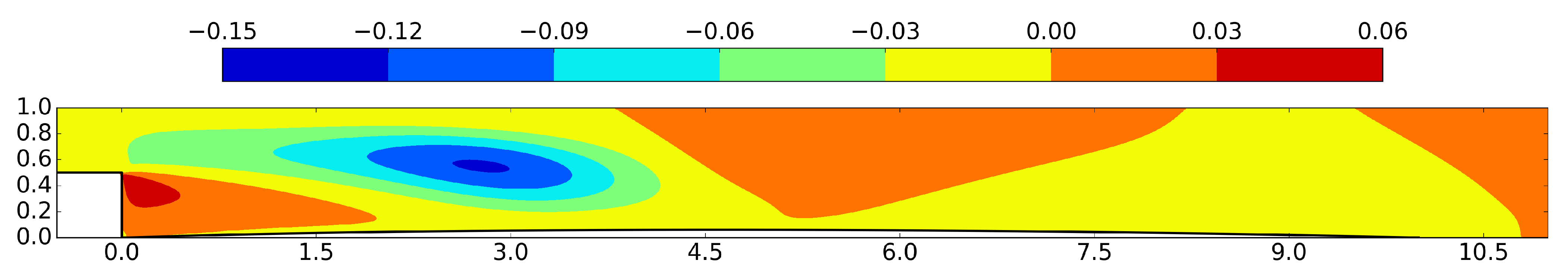
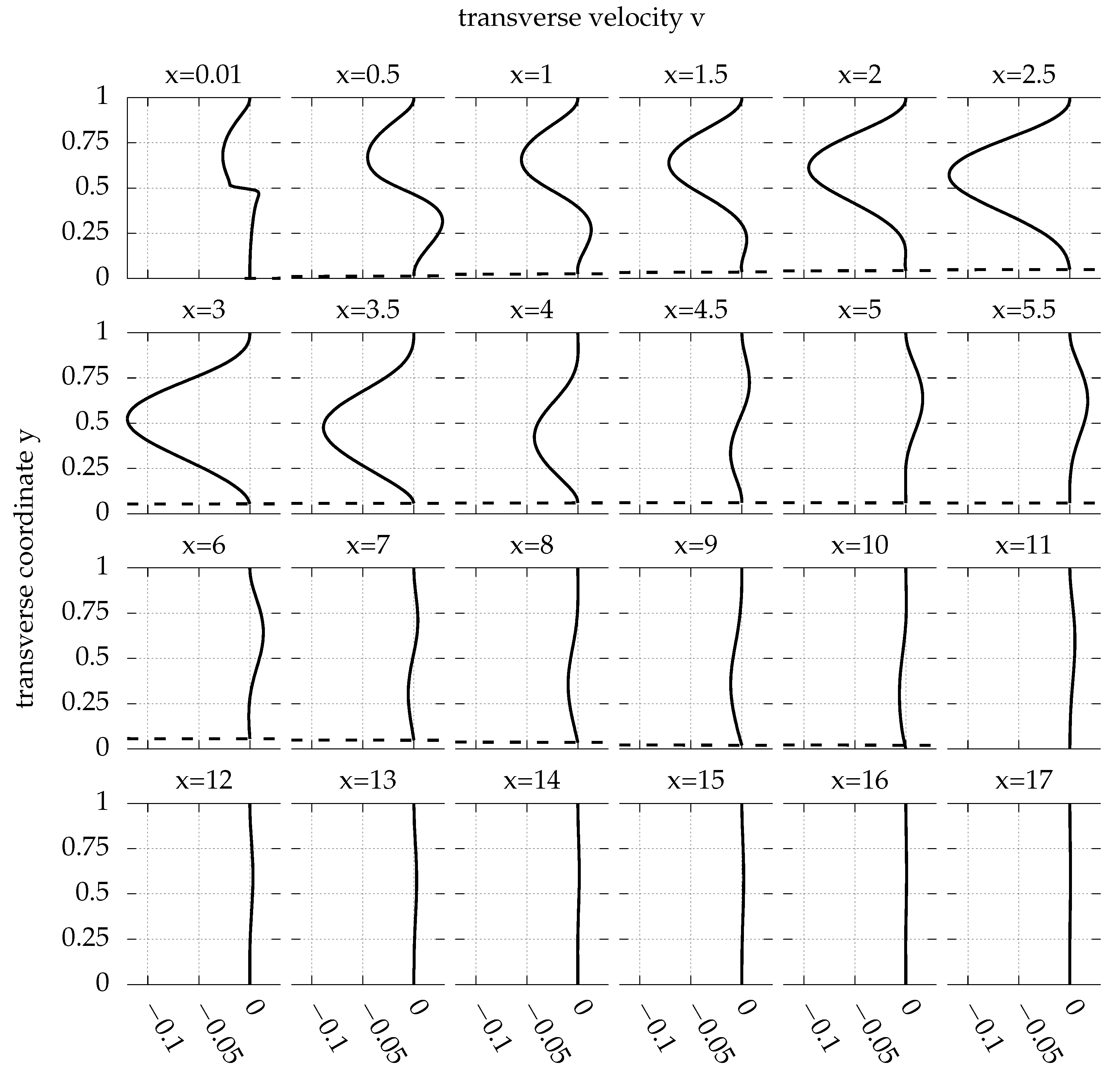
Due to the inertia of the flow, the expansion of the mainstream of the flow after the step position is not immediate, as shown by the longitudinal velocity contours of Figure 4 and the longitudinal velocity profiles of Figure 5. It develops downstream of the step and exhibits its major intensity approximately at the region , as shown in the transverse velocity contours of Figure 6 and the transverse velocity profiles of Figure 7.
The lower wall closed streamlines extend as far as , reducing by the uncontrolled separation length of magnitude (Section 3.1). The upper wall separation region vanishes. The transverse velocity profile zeroes at , indicating that the flow is developed at this point. Longitudinal velocity profiles (Figure 5) confirm the observation, as the velocity profile at this point is parabolic.
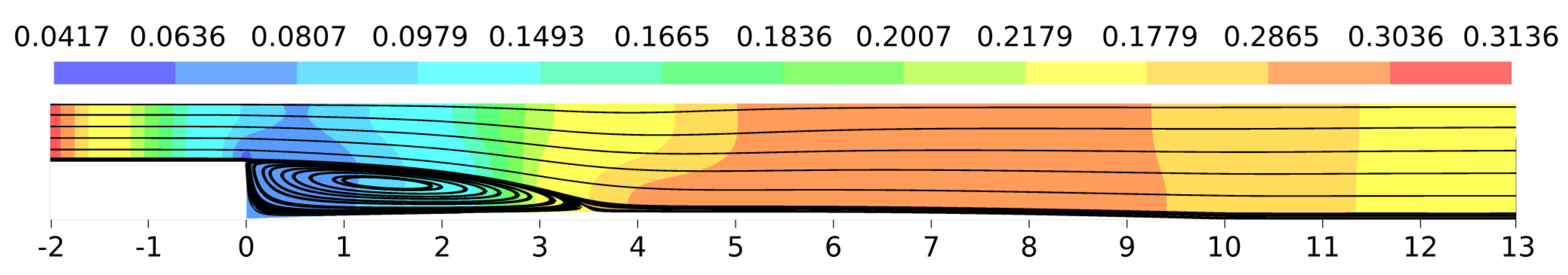
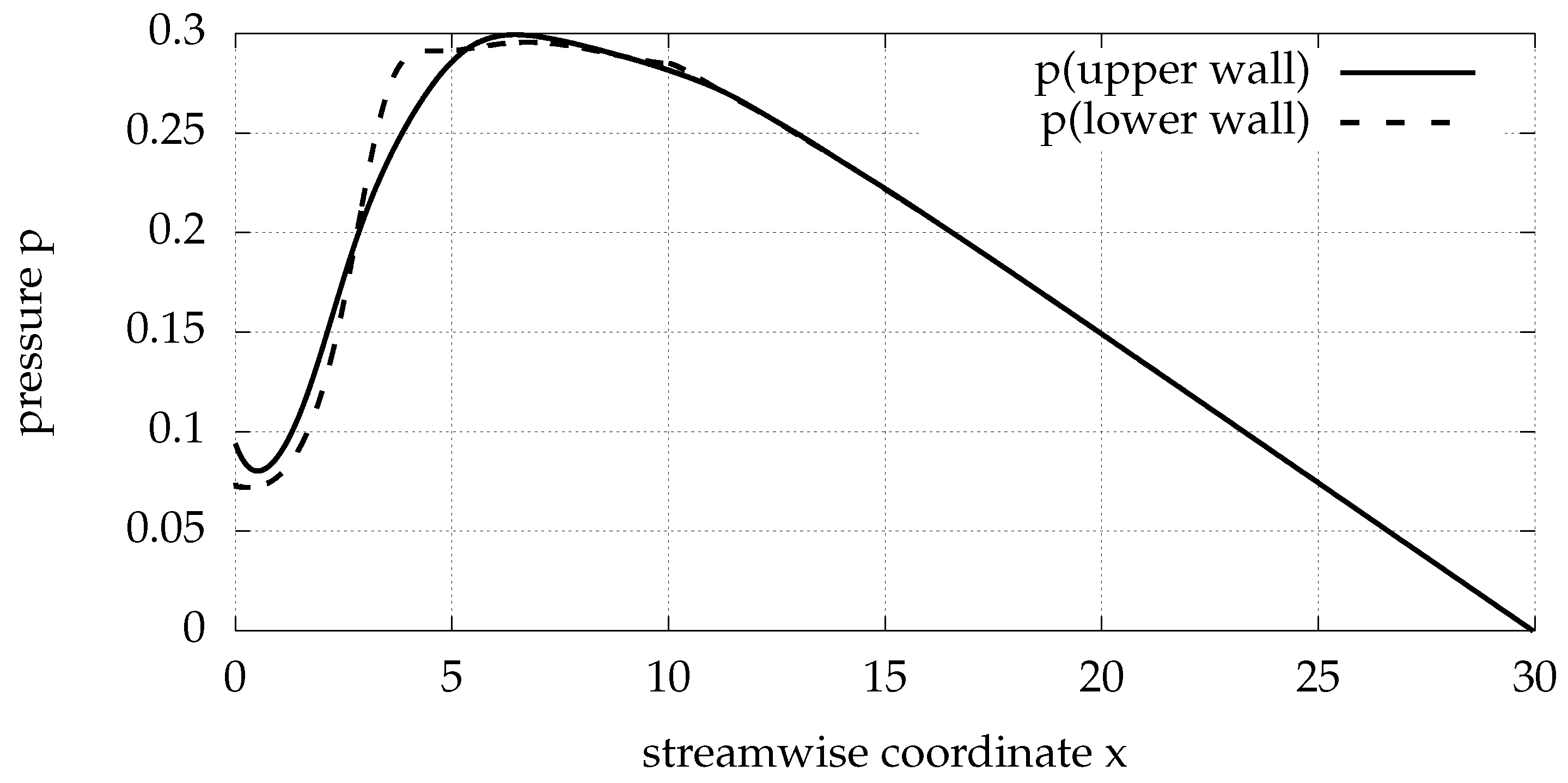
Due to the low velocity of the fluid under the inlet flow, at the lower wall bubble, the curvature of the streamlines is small. Hence, the pressure distribution is nearly uniform for each cross section (Figure 8) [46]. At the region the streamlines are slightly convex down. At this segment, the lower wall pressure is higher than the upper wall pressure with maximum surplus value , as shown in Figure 9. Pressure raises streamwise after the step, by the combined application of momentum and continuity equations and reaches its maximum close to the position where the major low recirculation region reaches its end [47]. After this position, the pressure drops streamwise due to the action of viscosity. These remarks are in accordance with the results of [30] for the analogous case for .
3.3. Unsteady Periodic Flow
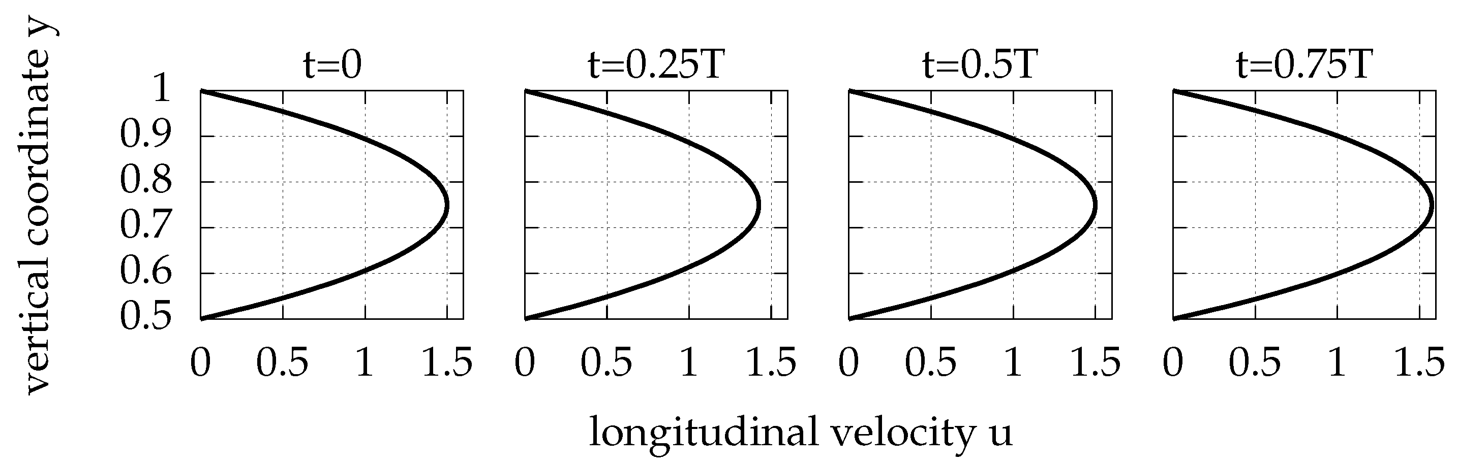
The periodic flow under the inflow velocity defined in Section 2.1, is computed as the subject of control of the next subsections. The amplitude of the flow oscillation is taken and the respective frequency of the flow is , following previous research [13]. The time varying parabolic inlet velocity profile for oscillation amplitude is depicted at Figure 10.
The detachment and reattachment positions under unsteady flow without control are shown in Figure 11. As fluid volume entering the BFS shrinks because of the decrease in the inlet velocity, the upper wall detachment position is moved downstream because of the reduced viscosity effects resulting from the lower velocity values. Meanwhile, the lower wall reattachment position is moved upstream due to the reduced inertia of the flow. Finally, the upper wall reattachment position is also moved upstream due to the upstream movement of the lower wall stagnation point. In the increasing phase of the inlet velocity, where the fluid volume inserting the geometry reaches its higher values, the remarks are reversed. The results are in good agreement with those of Mateescu et al. [13].
3.4. Active Control of Unsteady Periodic Flow
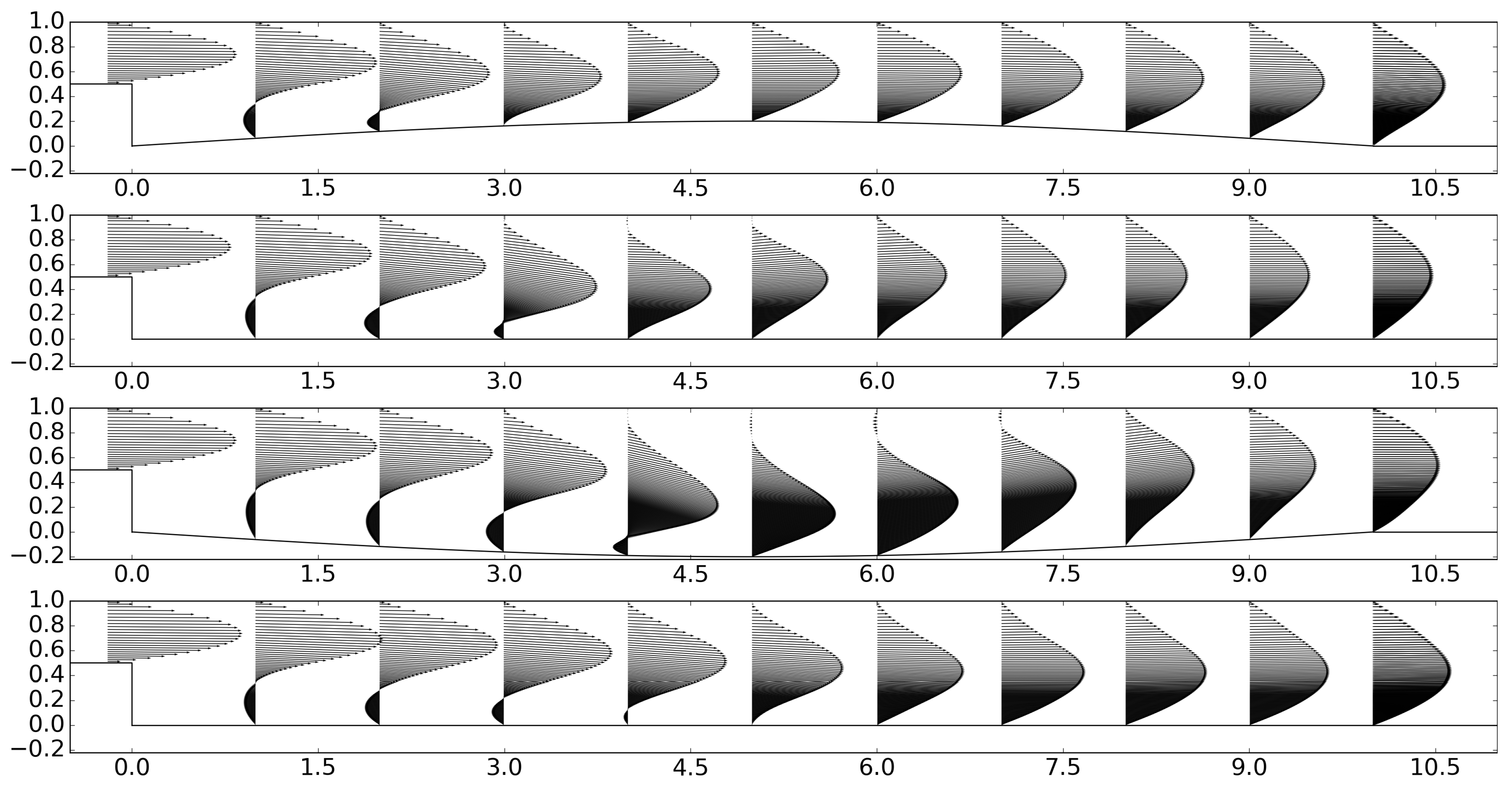
Aiming at controlling the flow of Section 3.3, the portion of the bottom wall downstream the step with length l is forced moving sinusoidally following Equation (3). For amplitude , frequency and length the evolution of the flow field in time is presented at Figure 12. The emergence and disappearance of the upper wall recirculation region and the fluctuation of the position of lower wall reattachment are visible.
As shown by evolution in time of the positions of detachment and reattachment, presented in Figure 13, the significant lowering of the bottom wall at the half period decreases the inclination of the lower wall stagnation line and increases its length. Therefore, pushes the lower wall reattachment position downstream. On the contrary, the maximum positive position of the oscillating portion of the bottom wall increases the inclination and decreases the length of the stagnation line, therefore causes the lower wall reattachment to move upstream. The upper wall backflow emerges more distantly from the step position and elongates, as the control surface moves downwards. In the second half of the period, where the control surface moves upwards and the inlet velocity increases, the upper wall bubble quickly vanishes. As a consequence of the significant amplitude of the oscillation of the control surface (), which is a fifth of the expanded duct cross-section, the flow is attached at the upper wall for half of the period.
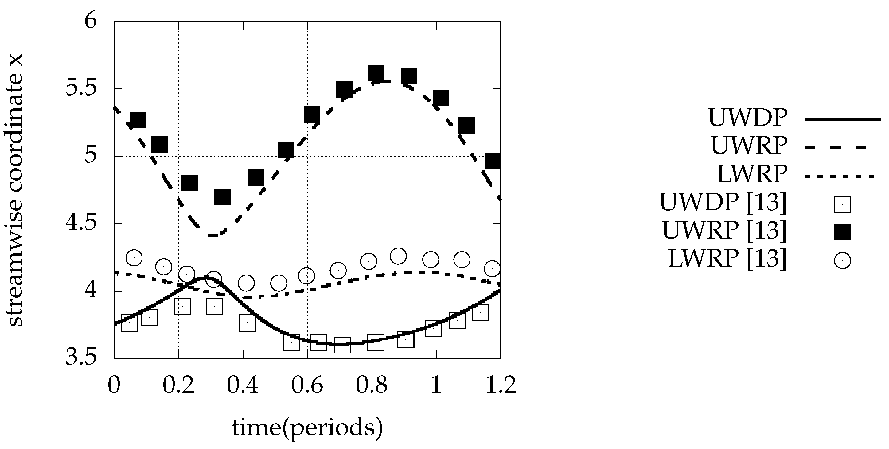
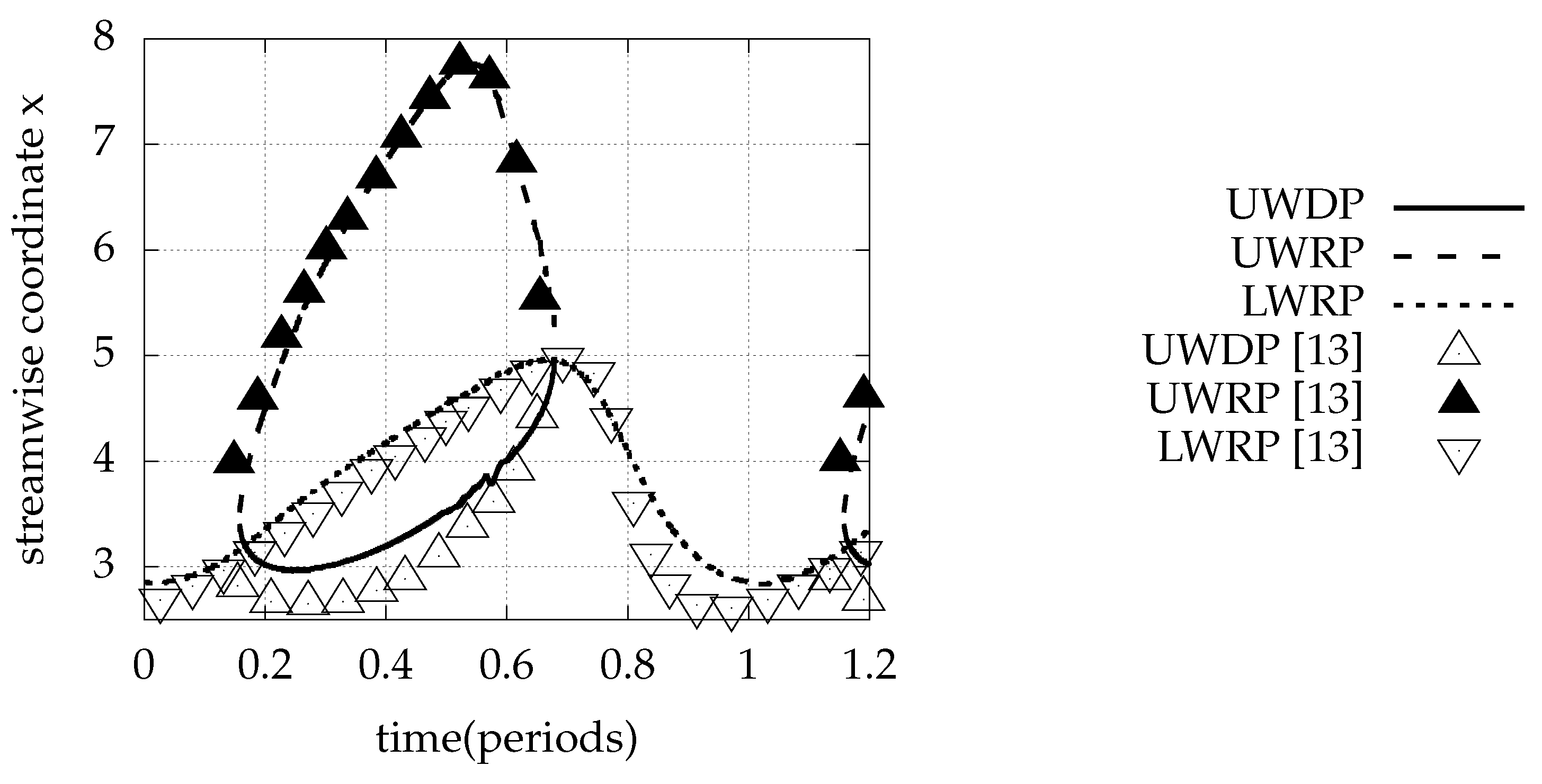
Comparing the positions of the separated zones, our results are close to those of Mateescu et al. [13]. The detachment positions computed with the immersed boundary method lays at most downstream of that computed with the body-fitted method. Upper wall reattachment positions during the cycle are in good agreement with those calculated by Mateescu et al. Lower wall reattachment position curves differ slightly before the end of the period. Current results are smoother at the time when the bottom wall bubble begins to extend downstream.
The effect of the frequency , the amplitude of the oscillation A and the length of the oscillating surface l is investigated by changing one at a time.
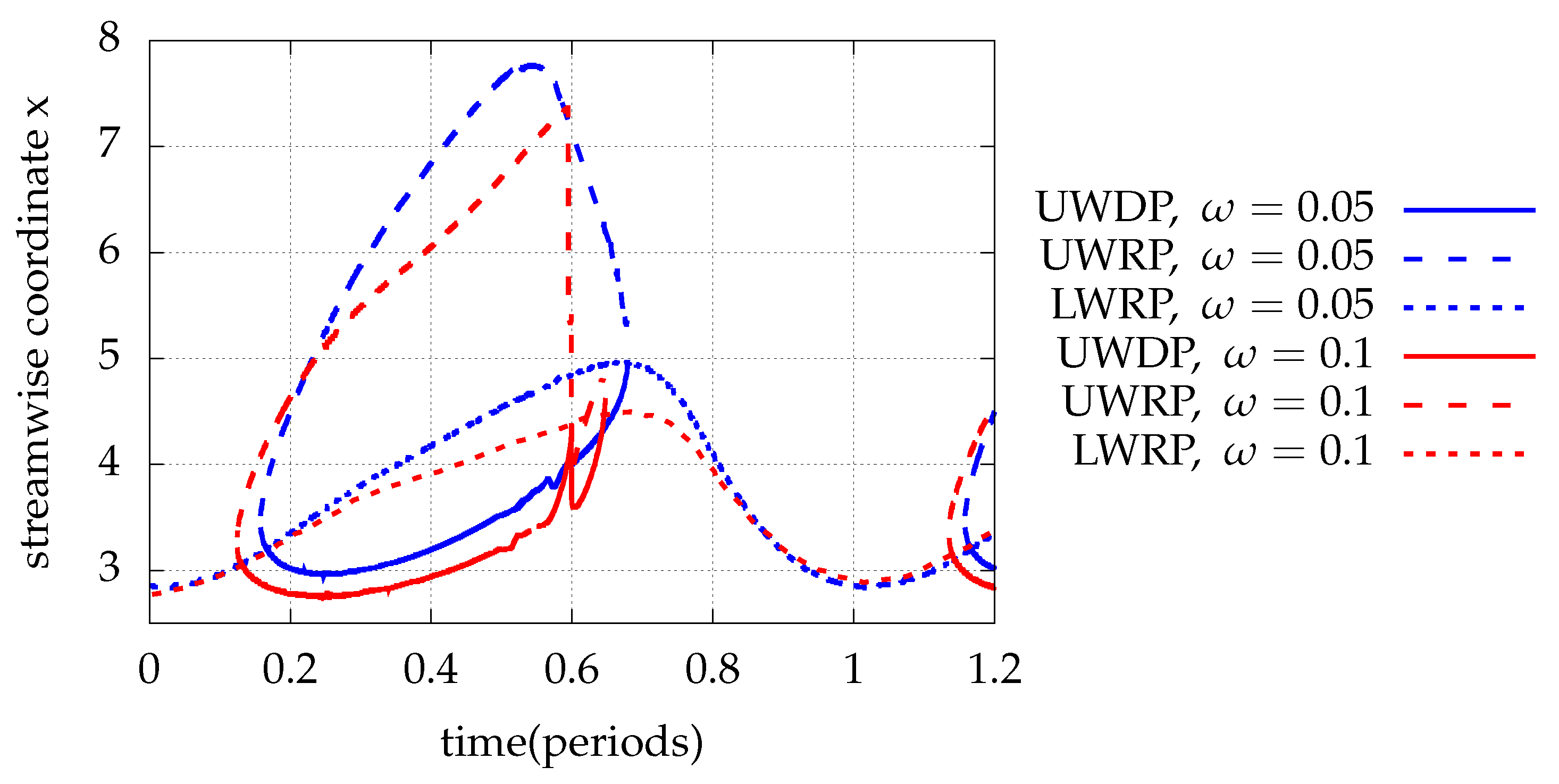
As seen in Figure 14, the increase in the frequency of the oscillation (, ) pushes upstream the upper and lower wall reattachment and also the upper wall detachment locations. The upper and lower wall recirculation oscillation amplitudes decrease with the higher frequency. Furthermore, the upper wall recirculation instantly vanishes and reappears for a small percentage of the period and also emerges earlier in the period for faster oscillating inlet velocity. This behavior arises probably due to a flow instability in the higher frequency in combination with the relatively large wall oscillation amplitude . These observations are in accordance with analogous research with body fitted methods [13].
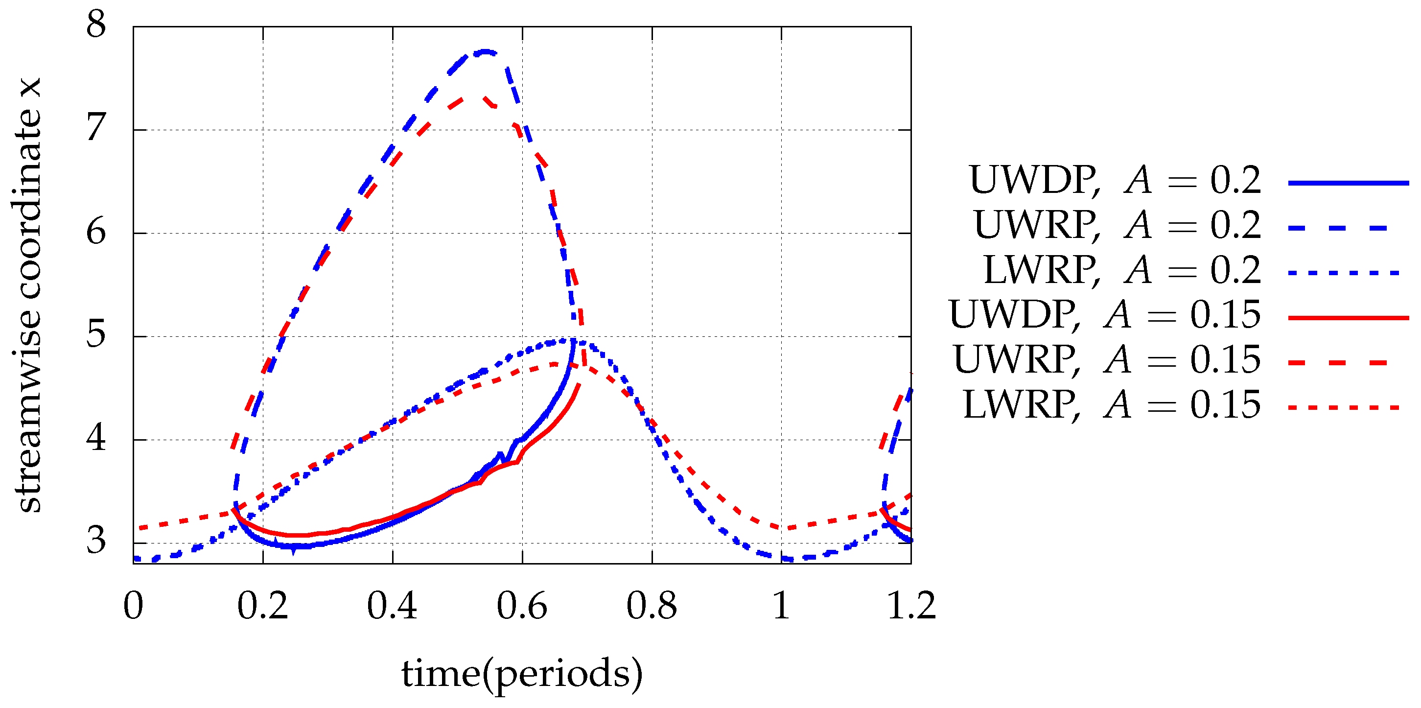
A decrease in the amplitude of oscillation of the moving portion of the bottom wall (, ) causes the reduction in the upper wall separation region length. It also causes the presence of the upper wall recirculation for larger portion of the period and to the downstream movement of the respective detachment position. Furthermore, it leads to the reduction in lower wall reattachment position oscillation amplitude (Figure 15). The less upper wall and lower wall bubble length fluctuations is directly related to the reduced oscillation amplitude of the control surface. The remarks of Mateescu et al. [13] are in agreement with the aforementioned.
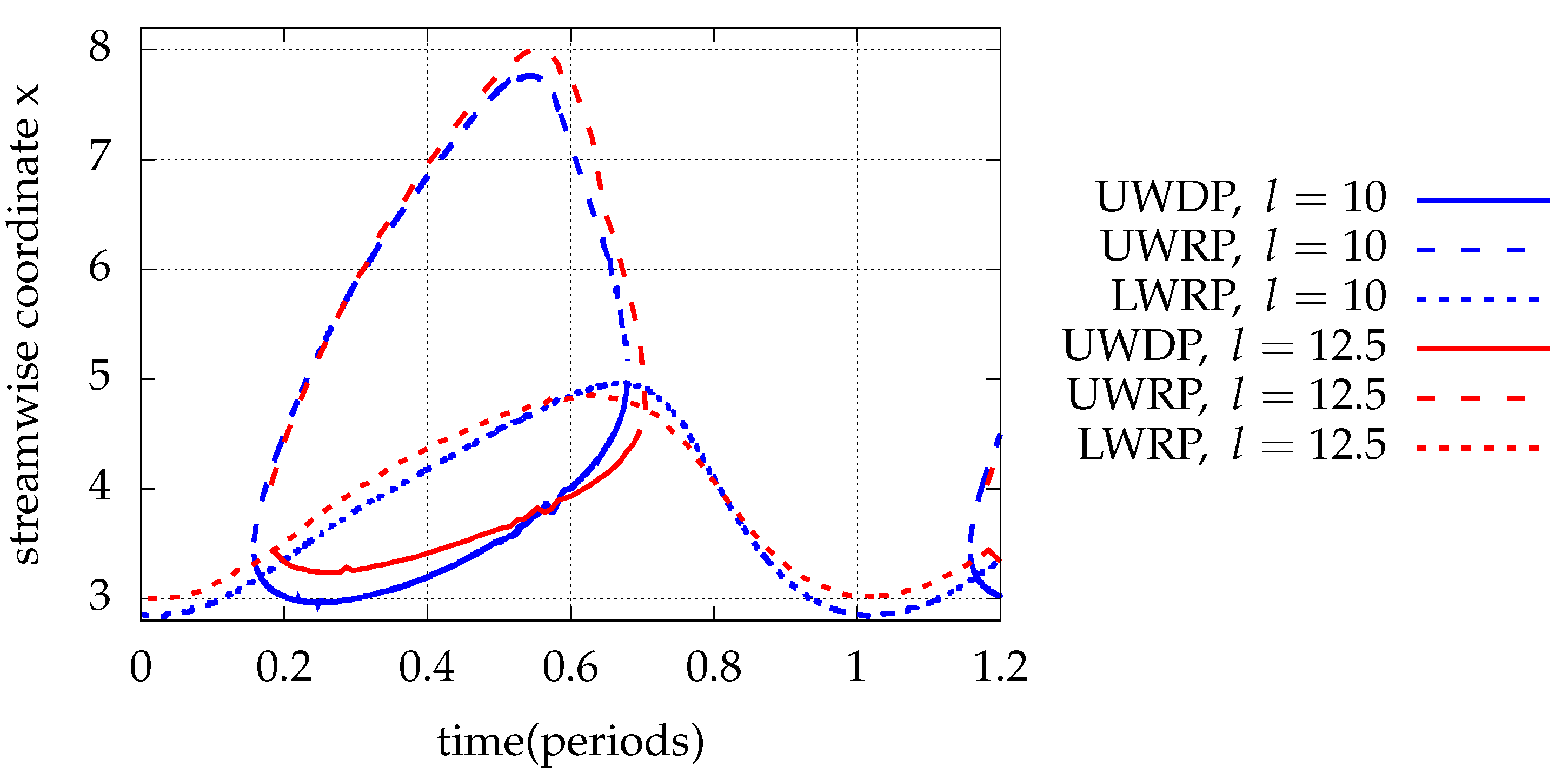
Finally, for the increase in the oscillating surface length (, ), the fluctuation of the bottom wall recirculation length and top wall detachment position decrease, while the presence of the upper wall recirculation extends in time, as suggested by Figure 16. This trend is attributed to the fact, that the lower wall stagnation point is more distant to the middle point of the control surface length, which exhibits maximum amplitude. Therefore, its vertical oscillation amplitude reduces and consequently its longitudinal oscillation amplitude also reduces.
3.5. Passive Control of Unsteady Periodic Flow via Elastic Membrane
On the purpose of controlling the flow computed in Section 3.3, we also employ an elastic membrane which follows Equation (4) with tension and with external pressure exerted at its outer side, . As for the steady case, the membrane parameters and are selected so that the maximum deformation of the membrane is retained at a low level () during the period. Additional objectives leading to the parameters’ values, are the external pressure to be of the same order of magnitude with the pressure exerted by the flow and the transmural pressure to be positive.
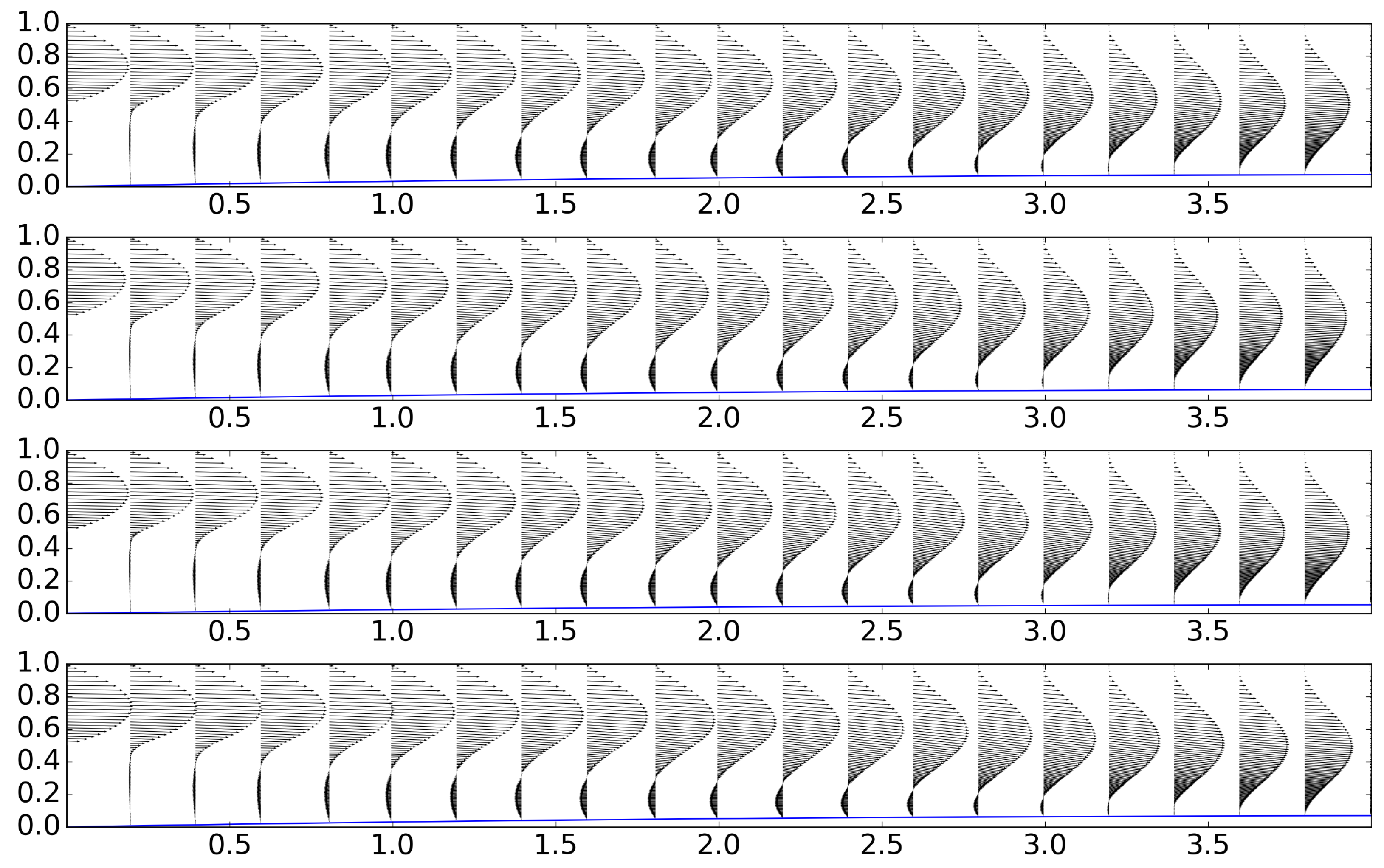
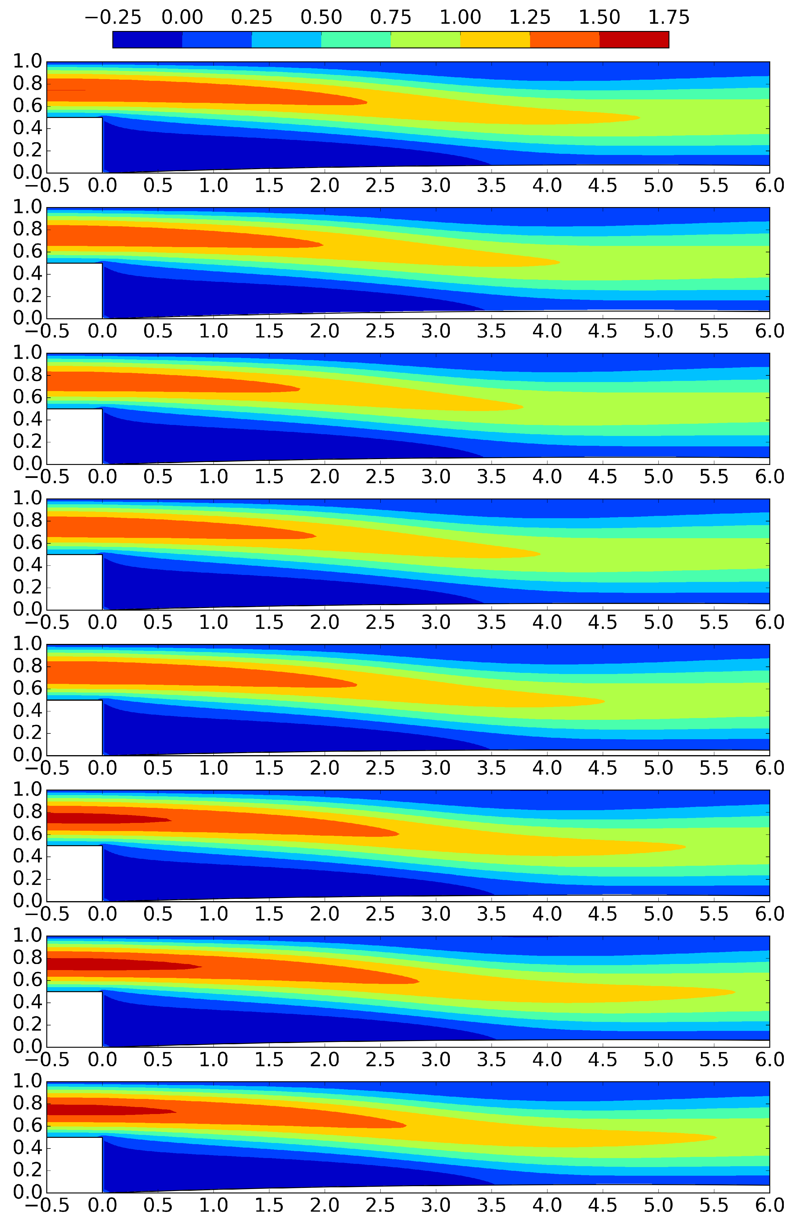
The interaction of the flow with the elastic membrane leads to the complete suppression of the upper wall recirculation as shown in the velocity profiles of Figure 17 and the longitudinal velocity contours of Figure 18. The free shear layer is identified by the set of transition points where longitudinal velocity changes sign.
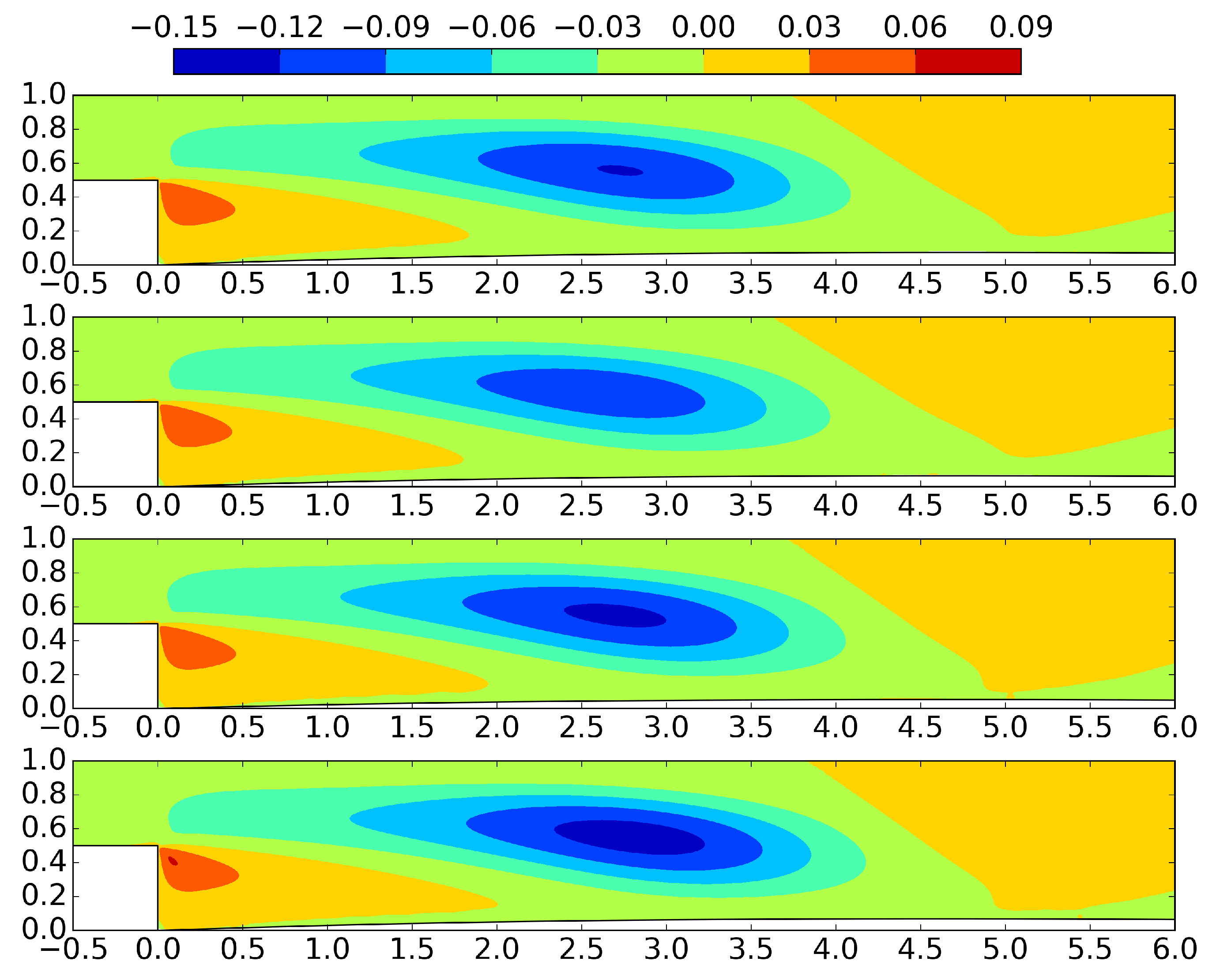
Inasmuch as a relatively stiff membrane is employed (), the membrane oscillation amplitude is restricted comparing to the active control of the previous subsection, as shown in Figure 17. In the longitudinal velocity contours exhibited in Figure 18, the oscillation of the inflow is observed. A no negative values region is noted at the upper wall, indicating absence of upper wall flow reversal. The lower wall recirculation region extension is indicated by the negative values zone. Following the free shear layer oscillation, the lower wall reattachment position is fluctuating around . In Figure 19, the transverse velocity contours suggest more intensive downstream motion at the region for , when the inlet fluid volume rate is maximum.
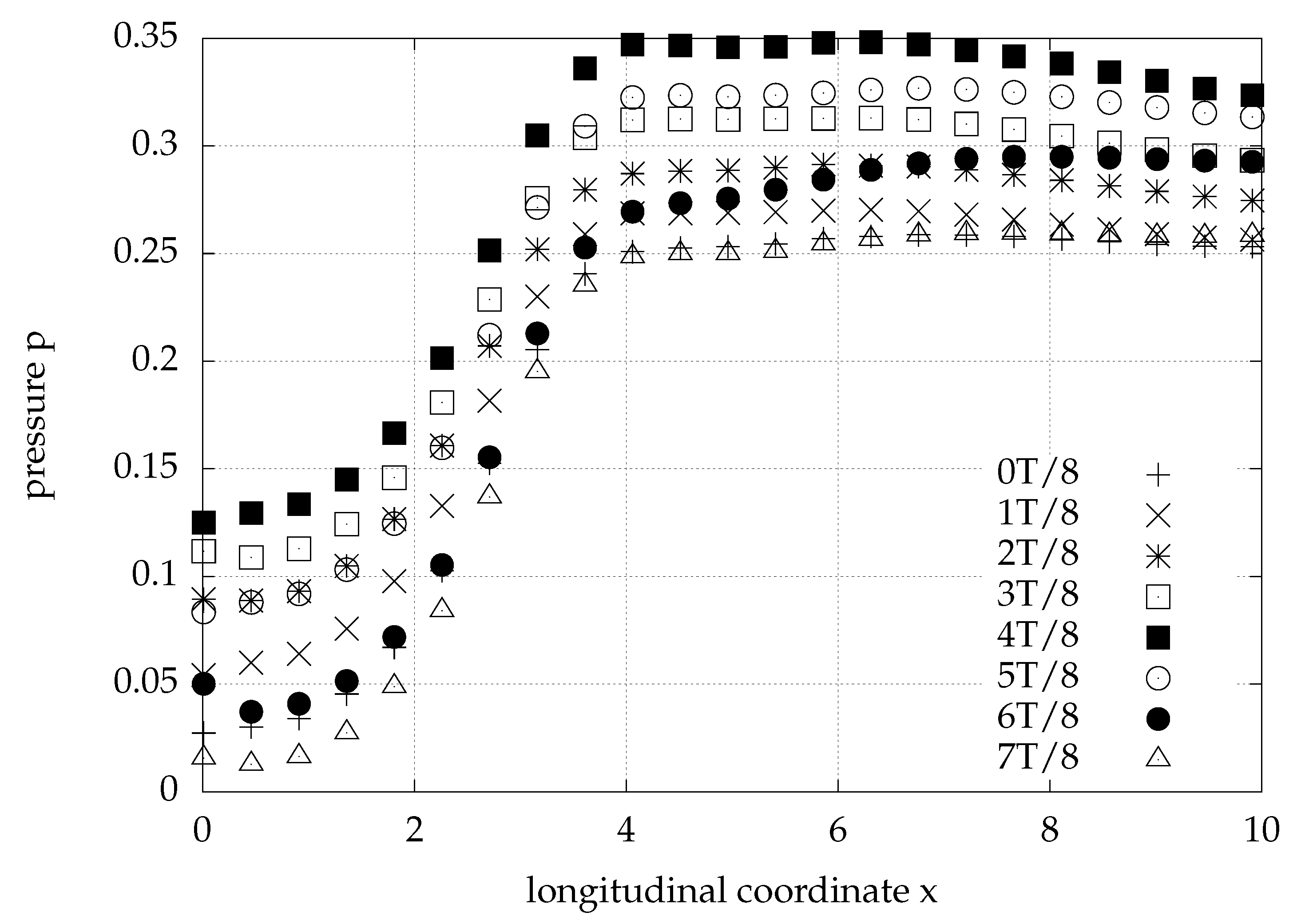
The induced pressure at the inner side of the membrane during the periodic inflow cycle is presented in Figure 20. As in the steady case (Figure 9), pressure recovers downstream of the step and is maximized at the longitudinal position close to the lower wall reattachment cross-section [47]. Downstream of the stagnation point, the pressure drops streamwise due to the action of frictional forces. The maximum pressure fluctuation emerges at and has the value .
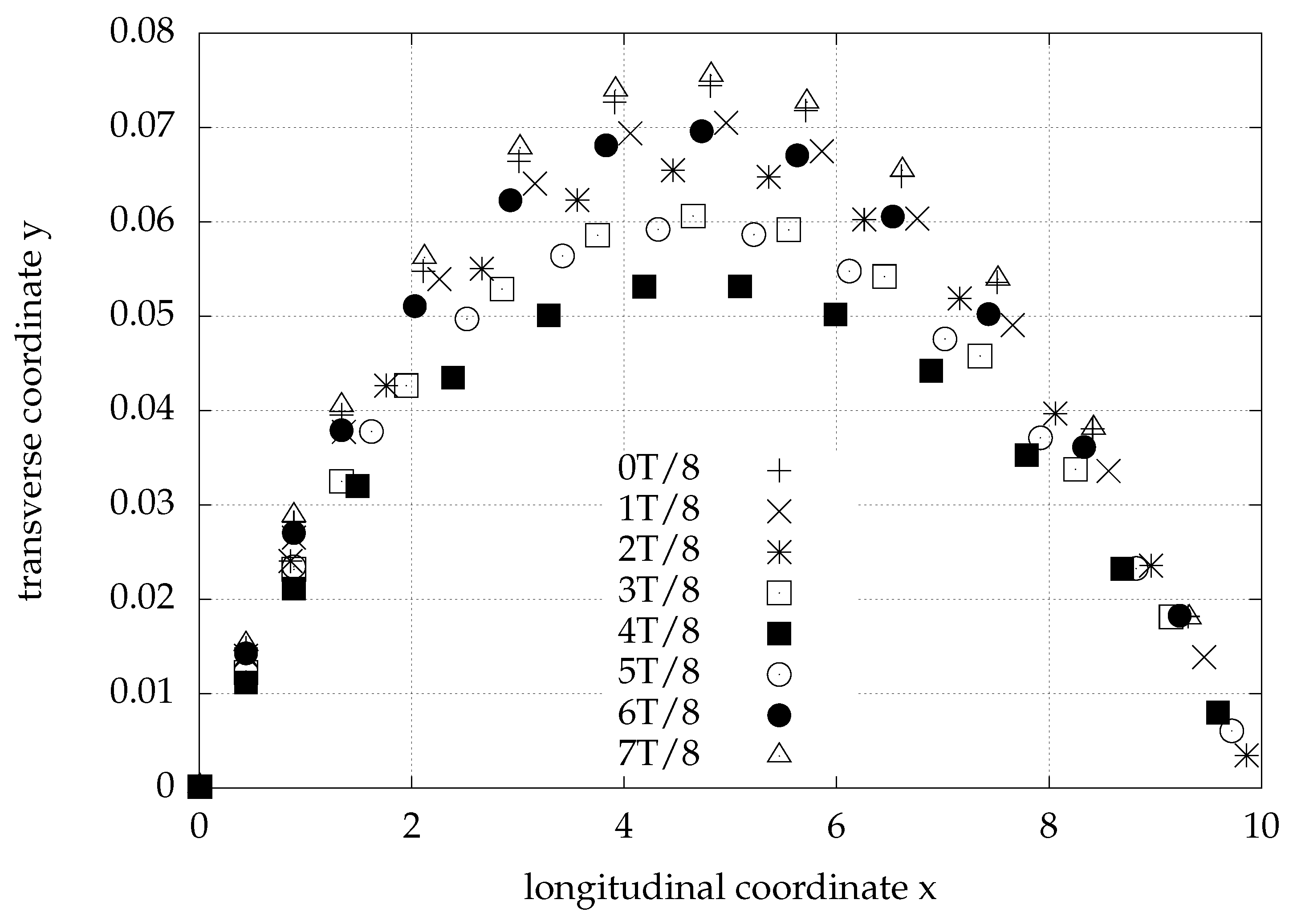
The corresponding membrane shape is presented in Figure 21. Membrane curve at the x-y plane is approximately that of a concave down parabola due to the relatively high values of its parameters chosen (tension, external pressure). The membrane displacement shows overall larger values for the instances in time where the inner pressure distribution on the membrane reaches its higher values. The largest membrane displacement occurs at due to the inner membrane pressure distribution, which exhibits noticeably lower mean value at the left half of its domain () and higher values at the right half (). The periodical motion of the membrane is a result of its interaction with the oscillating inlet flow. Through this interaction, the membrane inner pressure distributions are decided. The work of the membrane is produced by its oscillation along with the varying membrane inner pressure distribution.
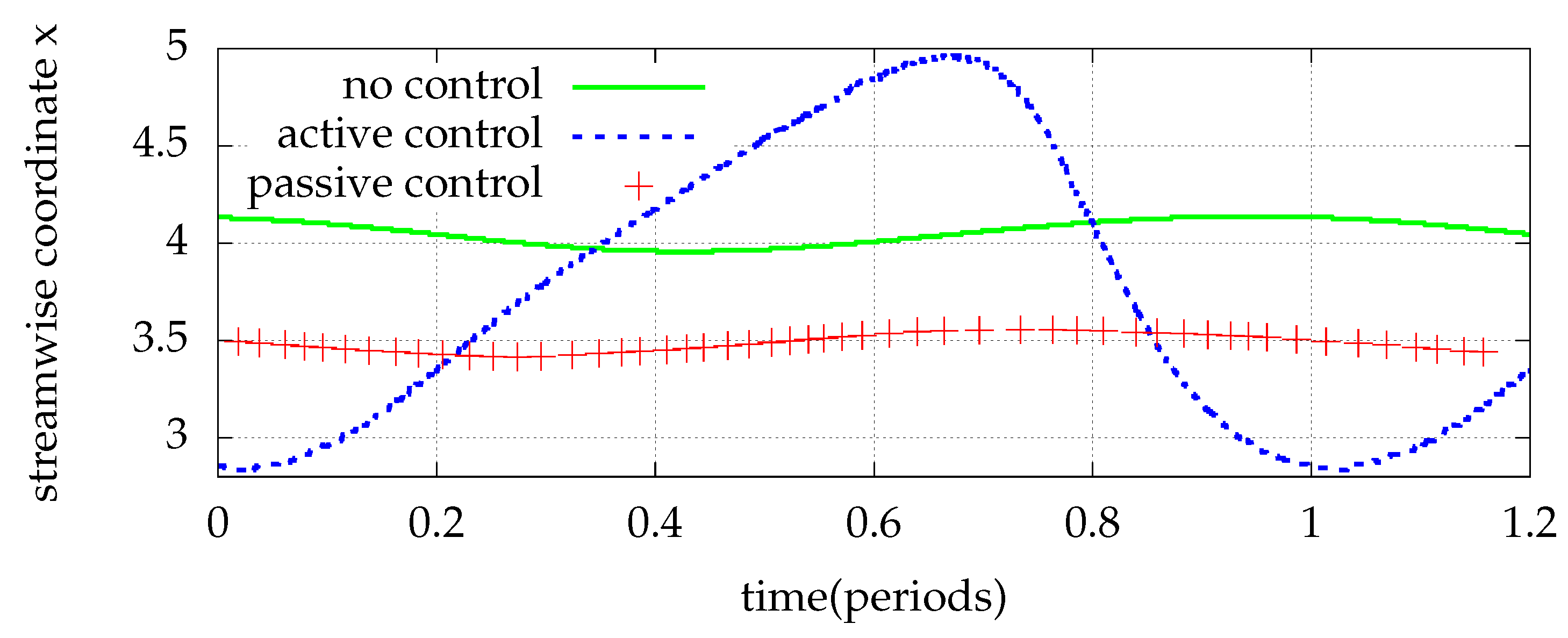
As Figure 22 suggests, the length of the lower wall separated zone is significantly smaller (), as its maximum value drops to nearly from for the flow without control. Moreover, small reduction in the fluctuation of its length is observed. The peak to peak fluctuation of for the without control case, drops to the value for the passive control case, i.e., a reduction is noted.
4. Conclusions
The immersed boundary method is implemented to compute the steady and unsteady periodic laminar flow over a backward facing step without and with control. The results are in close agreement with those of body fitted methods for the cases where such exist. Two techniques for the control of the flow are employed.
Aiming at establishing active control, a portion of the bottom wall downstream of the step is oscillating in a prescribed sinusoidal way. The effect of the frequency, the amplitude and the length of the oscillating surface on the longitudinal detachment and attachment positions and longitudinal extension of closed streamlines are examined. The effect of the length of the oscillating surface to the control of the flow over a BFS, has not been investigated before. Increase in the frequency transfers the occurrence of the upper wall recirculation bubble earlier during the period, a reduction in the oscillation amplitude of the surface reduces the upper wall recirculation length. Increase in the length of the control surface compresses the range of the upper wall detachment position and decreases the fluctuation of the position of lower wall stagnation point.
In the passive control setting, the same rigid control part of the bottom wall is substituted with an elastic membrane and the steady and unsteady fluid structure interaction problems are solved. This method of control is implemented for the first time for a flow over a backward facing step. As a result of the control, the upper wall recirculation region vanishes while the lower one is reduced both in steady and periodic cases. The fluctuation of the lower wall separation length is also shortened for the time varying case. A parametric study of the effect of the membrane parameters to the separation is a further investigation objective.
Author Contributions
I.M., C.M. and S.T. provided equal contributions to this research paper. All authors have read and agreed to the published version of the manuscript.
Funding
This research was co-funded by the European Union and Greek national funds through the Operational Program Competitiveness, Entrepreneurship and Innovation, under the call RESEARCH–CREATE–INNOVATE (project code: T1EDK-01366, MIS: 5032787).
Data Availability Statement
Data sharing is not applicable to this article.
Acknowledgments
We acknowledge Kyriakos Giannakoglou at the National Technical University of Athens (NTUA) for kindly granting us the opportunity and support to perform the simulations on the NTUA Parallel CFD and Optimization Unit cluster.
Conflicts of Interest
The authors declare no conflict of interest.
References
- Emami-Naeini, A.; McCabe, S.; de Roover, D.; Ebert, J.; Kosut, R. Active Control of Flow Over a Backward-Facing Step. In Proceedings of the 44th IEEE Conference on Decision and Control, Seville, Spain, 12–15 December 2005; pp. 7366–7371. [Google Scholar]
- Sakuraba, K.; Fukazawa, K.; Sano, M. Control of Turbulent Channel Flow over a Backward-Facing Step by Suction or Injection. Heat Transfer 2004, 33, 490–504. [Google Scholar]
- Chen, L.; Asai, K.; Nonomura, T.; Xi, G.; Liu, T. A review of Backward-Facing Step (BFS) flow mechanisms, heat transfer and control. Therm. Sci. Eng. Prog. 2018, 6, 194–216. [Google Scholar] [CrossRef]
- Wang, B.; Li, H. POD analysis of flow over a backward-facing step forced by right-angle-shaped plasma actuator. SpringerPlus 2016, 5, 795. [Google Scholar] [CrossRef] [PubMed] [Green Version]
- You, D.; Moin, P. Active control of flow separation over an airfoil using synthetic jets. J. Fluids Struct. 2008, 24, 1349–1357. [Google Scholar] [CrossRef]
- Ma, X.; Schröder, A. Analysis of flapping motion of reattaching shear layer behind a two-dimensional backward-facing step. Phys. Fluids 2017, 29, 115104. [Google Scholar] [CrossRef]
- Tihon, J.; Penkavova, V.; Pantzali, M. The effect of inlet pulsations on the backward-facing step flow. Eur. J. Mech. B/Fluids 2010, 29, 224–235. [Google Scholar] [CrossRef]
- Kapiris, P.; Mathioulakis, D. Experimental study of vortical structures in a periodically perturbed flow over a backward-facing step. Int. J. Heat Fluid Flow 2014, 47, 101–112. [Google Scholar] [CrossRef]
- Morioka, T.; Honami, S. Dynamic Characteristics in a Control System of Backward Facing Step Flow by Vortex Generator Jets. In Proceedings of the 2nd AIAA Flow Control Conference, Portland, Oregon, 28 June–1 July 2004. [Google Scholar]
- Chun, K.; Sung, H. Control of turbulent separated flow over a backward-facing step by local forcing. Exp. Fluids 1996, 21, 417–426. [Google Scholar] [CrossRef]
- Gautier, N.; Aider, J.L. Control of the separated flow downstream of a backward-facing step using visual feedback. Proc. R. Soc. A Math. Phys. Eng. Sci. 2013, 469, 20130404. [Google Scholar] [CrossRef]
- Mateescu, D.; Venditti, D.A. Unsteady confined viscous flows with oscillating walls and multiple separation regions over a downstream-facing step. J. Fluids Struct. 2001, 15, 1187–1205. [Google Scholar] [CrossRef]
- Mateescu, D.; Muñoz, M.; Scholz, O. Analysis of unsteady confined viscous flows with variable inflow velocity and oscillating walls. J. Fluids Eng. 2010, 132, 041105. [Google Scholar] [CrossRef] [Green Version]
- Graff, K. Wave Motion in Elastic Solids; Dover Publications: New York, NY, USA, 1975. [Google Scholar]
- Tsangaris, S.; Pappou, T. Flow investigation in deformable arteries. In Intra and Extracorporeal Cardiovascular Fluid Dynamics; Verdonck, P., Perktold, K., Eds.; WIT Press: Boston, MA, USA, 2000; Volume 33, pp. 291–332. [Google Scholar]
- Luo, X.Y.; Pedley, T.J. A Numerical Simulation of Steady Flow in a 2-D Collapsible Channel. J. Fluids Struct. 1995, 9, 149–174. [Google Scholar] [CrossRef]
- Gregory, A.L.; Agarwal, A.; Lasenby, J. An experimental investigation to model wheezing in lungs. R. Soc. Open Sci. 2021, 8, 201951. [Google Scholar] [CrossRef] [PubMed]
- Matthews, L.A.; Greaves, D.M.; Williams, C.J.K. Numerical simulation of viscous flow interaction with an elastic membrane. Int. J. Numer. Methods Fluids 2008, 57, 1577–1602. [Google Scholar] [CrossRef]
- Luo, X.Y.; Pedley, T.J. A numerical simulation of unsteady flow in a two-dimensional collapsible channel. J. Fluid Mech. 1996, 314, 191–225. [Google Scholar] [CrossRef]
- Huang, L. Viscous flutter of a finite elastic membrane in poiseuille flow. J. Fluids Struct. 2001, 15, 1061–1088. [Google Scholar] [CrossRef]
- Peskin, C.S. Flow patterns around heart valves: A numerical method. J. Comput. Phys. 1972, 10, 252–271. [Google Scholar] [CrossRef]
- Saleel, A.C.; Shaija, A.; Jayaraj, S. On Simulation of Backward Facing Step Flow Using Immersed Boundary Method. Am. J. Fluid Dyn. 2013, 3, 9–19. [Google Scholar]
- Yang, D.; He, S.; Shen, L.; Luo, X. Large eddy simulation coupled with immersed boundary method for turbulent flows over a backward facing step. Proc. Inst. Mech. Eng. Part J. Mech. Eng. Sci. 2021, 235, 2705–2714. [Google Scholar] [CrossRef]
- Ge, L.; Sotiropoulos, F. A numerical method for solving the 3D unsteady incompressible Navier—Stokes equations in curvilinear domains with complex immersed boundaries. J. Comput. Phys. 2007, 225, 1782–1809. [Google Scholar] [CrossRef] [Green Version]
- Borazjani, I.; Ge, L.; Sotiropoulos, F. Curvilinear immersed boundary method for simulating fluid structure interaction with complex 3D rigid bodies. J. Comput. Phys. 2008, 227, 7587–7620. [Google Scholar] [CrossRef] [Green Version]
- Gilmanov, A.; Le, T.B.; Sotiropoulos, F. A numerical approach for simulating fluid structure interaction of flexible thin shells undergoing arbitrarily large deformations in complex domains. J. Comput. Phys. 2015, 300, 814–843. [Google Scholar] [CrossRef] [Green Version]
- Mittal, R.; Iaccarino, G. Immersed boundary methods. Annu. Rev. Fluid Mech. 2005, 37, 239–261. [Google Scholar] [CrossRef] [Green Version]
- Armaly, B.F.; Durst, F.; Pereira, J.C.F.; Schönung, B. Experimental and theoretical investigation of backward-facing step flow. J. Fluid Mech. 1983, 127, 473–496. [Google Scholar] [CrossRef]
- Kim, J.; Moin, P. Application of a fractional-step method to incompressible Navier-Stokes equations. J. Comput. Phys. 1985, 59, 308–323. [Google Scholar] [CrossRef]
- Gartling, D.K. A test problem for outflow boundary conditions—Flow over a backward-facing step. Int. J. Numer. Methods Fluids 1990, 11, 953–967. [Google Scholar] [CrossRef]
- Sohn, J.L. Evaluation of FIDAP on some classical laminar and turbulent benchmarks. Int. J. Numer. Methods Fluids 1988, 8, 1469–1490. [Google Scholar] [CrossRef]
- Pappou, T.; Tsangaris, S. Development of an artificial compressibility methodology using flux vector splitting. Int. J. Numer. Methods Fluid Mech. 1997, 25, 523–545. [Google Scholar] [CrossRef]
- Fernández-Feria, R.; Sanmiguel-Rojas, E. An explicit projection method for solving incompressible flows driven by a pressure difference. Comput. Fluids 2004, 33, 463–483. [Google Scholar] [CrossRef]
- Angelidis, D.; Chawdhary, S.; Sotiropoulos, F. Unstructured Cartesian refinement with sharp interface immersed boundary method for 3D unsteady incompressible flows. J. Comput. Phys. 2016, 325, 272–300. [Google Scholar] [CrossRef] [Green Version]
- Yang, H.Q.; Habchi, S.D.; Przekwas, A.J. General strong conservation formulation of Navier-Stokes equations in nonorthogonal curvilinear coordinates. AIAA J. 1994, 32, 936–941. [Google Scholar] [CrossRef]
- Gilmanov, A.; Sotiropoulos, F. A hybrid Cartesian/immersed boundary method for simulating flows with 3D, geometrically complex, moving bodies. J. Comput. Phys. 2005, 207, 457–492. [Google Scholar] [CrossRef]
- George, P.; Borouchaki, H. Delaunay Triangulation and Meshing: Application to Finite Elements; Hermès: Paris, France, 1998. [Google Scholar]
- Kang, S.K. Numerical Modeling of Turbulent Flows in Arbitrarily Complex Natural Streams. Ph.D. Thesis, University of Minnesota, Minneapolis, MN, USA, 2010. [Google Scholar]
- Calderer, A.; Kang, S.; Sotiropoulos, F. Level set immersed boundary method for coupled simulation of air/water interaction with complex floating structures. J. Comput. Phys. 2014, 277, 201–227. [Google Scholar] [CrossRef] [Green Version]
- Patankar, S.V.; Spalding, D.B. A calculation procedure for heat, mass and momentum transfer in three-dimensional parabolic flows. Int. J. Heat Mass Transf. 1972, 15, 1787–1806. [Google Scholar] [CrossRef]
- Kang, S.; Lightbody, A.; Hill, C.; Sotiropoulos, F. High-resolution numerical simulation of turbulence in natural waterways. Adv. Water Resour. 2011, 34, 98–113. [Google Scholar] [CrossRef]
- Saad, Y.; Schultz, M.H. GMRES: A Generalized Minimal Residual Algorithm for Solving Nonsymmetric Linear Systems. SIAM J. Sci. Stat. Comput. 1986, 7, 856–869. [Google Scholar] [CrossRef] [Green Version]
- Knoll, D.A.; Keyes, D.E. Jacobian-free Newton–Krylov methods: A survey of approaches and applications. J. Comput. Phys. 2004, 193, 357–397. [Google Scholar] [CrossRef] [Green Version]
- VFS—WIND Virtual Flow Simulator. Available online: https://safl-cfd-lab.github.io/VFS-Wind/ (accessed on 10 January 2021).
- Press, W.H.; Teukolsky, S.A.; Vetterling, W.T.; Flannery, B.P. Numerical Recipes 3rd Edition: The Art of Scientific Computing; Cambridge University Press: Cambridge, UK, 2007. [Google Scholar]
- Greitzer, E.; Tan, C.; Graf, M. Internal Flow: Concepts and Applications; Cambridge Engine Technology Series; Cambridge University Press: Cambridge, UK, 2007. [Google Scholar]
- Spurk, J.H.; Aksel, N. Fluid Mechanics, 2nd ed.; Springer: Berlin/Heidelberg, Germany, 2008. [Google Scholar]
Figure 1.
Backward facing step with portion l of moving bottom wall. The inlet lies at and the outlet at .
Figure 1.
Backward facing step with portion l of moving bottom wall. The inlet lies at and the outlet at .

Figure 2.
The backward facing step under steady inflow, with control portion of elastic membrane bottom wall with and , for . The maximum membrane displacement arrow emerges at and has the value . Reattachment of the flow occurs at (indicated by the dashed line).
Figure 2.
The backward facing step under steady inflow, with control portion of elastic membrane bottom wall with and , for . The maximum membrane displacement arrow emerges at and has the value . Reattachment of the flow occurs at (indicated by the dashed line).

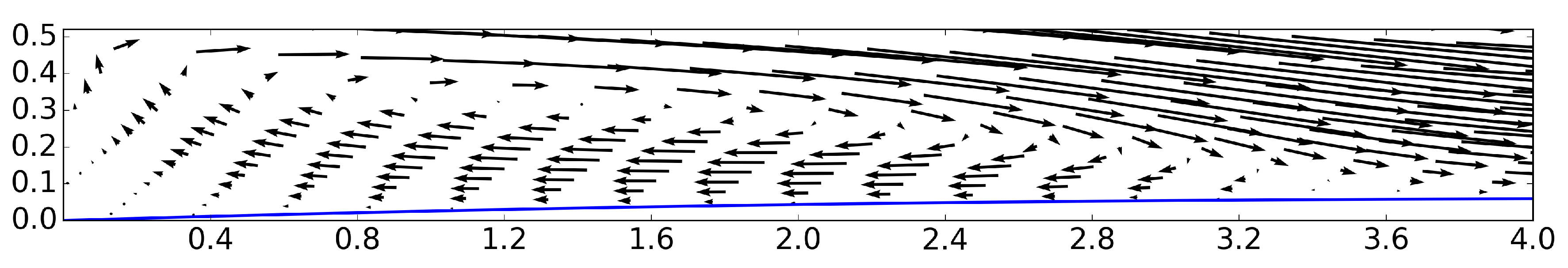
Figure 3.
Backward facing step under steady inflow, with control portion of elastic membrane bottom wall with and . Detail of the lower wall recirculation region for and .
Figure 3.
Backward facing step under steady inflow, with control portion of elastic membrane bottom wall with and . Detail of the lower wall recirculation region for and .

Figure 4.
Backward facing step under steady inflow, with control portion of elastic membrane bottom wall with and . Longitudinal velocity contour plot for . The lower reattachement position is emphasized by the dashed line.
Figure 4.
Backward facing step under steady inflow, with control portion of elastic membrane bottom wall with and . Longitudinal velocity contour plot for . The lower reattachement position is emphasized by the dashed line.

Figure 5.
Longitudinal velocity profiles for successive positions x downstream of the step, for BFS with control portion of elastic membrane bottom wall, with and , under steady inflow at (). The membrane shape is depicted also in non-dimensional units at the bottom (dashed line).
Figure 5.
Longitudinal velocity profiles for successive positions x downstream of the step, for BFS with control portion of elastic membrane bottom wall, with and , under steady inflow at (). The membrane shape is depicted also in non-dimensional units at the bottom (dashed line).

Figure 6.
Backward facing step under steady inflow, with control portion of elastic membrane bottom wall with and . Transverse velocity contour plot for .
Figure 6.
Backward facing step under steady inflow, with control portion of elastic membrane bottom wall with and . Transverse velocity contour plot for .

Figure 7.
Transverse velocity profiles for successive positions x downstream the step, for BFS with control portion of elastic membrane bottom wall, with and , at steady flow with (). The membrane shape is also depicted in non-dimensional units at the bottom (dashed line).
Figure 7.
Transverse velocity profiles for successive positions x downstream the step, for BFS with control portion of elastic membrane bottom wall, with and , at steady flow with (). The membrane shape is also depicted in non-dimensional units at the bottom (dashed line).

Figure 8.
Pressure contours and streamlines for BFS with control portion of elastic membrane bottom wall, with and , at steady flow with for .
Figure 8.
Pressure contours and streamlines for BFS with control portion of elastic membrane bottom wall, with and , at steady flow with for .

Figure 9.
Pressure distribution at lower and upper walls downstream the step for BFS with control portion of elastic membrane bottom wall, with and , at steady flow with .
Figure 9.
Pressure distribution at lower and upper walls downstream the step for BFS with control portion of elastic membrane bottom wall, with and , at steady flow with .

Figure 10.
Inflow velocity profiles for four time instances during the period (Equation (1)). The oscillation amplitude is .
Figure 10.
Inflow velocity profiles for four time instances during the period (Equation (1)). The oscillation amplitude is .

Figure 11.
Upper wall detachment position (UWDP) and upper and lower wall reattachment positions (UWRP, LWRP) for unsteady periodic inflow with , , and without control (). Comparison with results of Mateescu et al. [13] is presented.
Figure 11.
Upper wall detachment position (UWDP) and upper and lower wall reattachment positions (UWRP, LWRP) for unsteady periodic inflow with , , and without control (). Comparison with results of Mateescu et al. [13] is presented.

Figure 12.
Computed velocity fields for , , , , respectively, during a period T, for prescribed motion of the control surface with , , and . The inflow is oscillating with . The Reynolds number is 400.
Figure 12.
Computed velocity fields for , , , , respectively, during a period T, for prescribed motion of the control surface with , , and . The inflow is oscillating with . The Reynolds number is 400.

Figure 13.
Upper wall detachment position (UWDP) and upper and lower wall reattachment positions (UWRP, LWRP) for unsteady periodic inflow with and and oscillating part of the bottom wall with , , . Comparison with results of Mateescu et al. [13] is presented.
Figure 13.
Upper wall detachment position (UWDP) and upper and lower wall reattachment positions (UWRP, LWRP) for unsteady periodic inflow with and and oscillating part of the bottom wall with , , . Comparison with results of Mateescu et al. [13] is presented.

Figure 14.
Upper wall detachment position (UWDP) and upper and lower wall reattachment positions (UWRP, LWRP) for unsteady periodic inflow with and and oscillating part of the bottom wall with , , . Comparison with results for .
Figure 14.
Upper wall detachment position (UWDP) and upper and lower wall reattachment positions (UWRP, LWRP) for unsteady periodic inflow with and and oscillating part of the bottom wall with , , . Comparison with results for .

Figure 15.
Upper wall detachment position (UWDP) and upper and lower wall reattachment positions (UWRP, LWRP) for unsteady periodic inflow with and and oscillating part of the bottom wall with , , . Comparison with results for .
Figure 15.
Upper wall detachment position (UWDP) and upper and lower wall reattachment positions (UWRP, LWRP) for unsteady periodic inflow with and and oscillating part of the bottom wall with , , . Comparison with results for .

Figure 16.
Upper wall detachment position (UWDP) and upper and lower wall reattachment positions (UWRP, LWRP) for unsteady periodic inflow with and and oscillating part of the bottom wall with , , . Comparison with results for .
Figure 16.
Upper wall detachment position (UWDP) and upper and lower wall reattachment positions (UWRP, LWRP) for unsteady periodic inflow with and and oscillating part of the bottom wall with , , . Comparison with results for .

Figure 17.
Computed velocity fields for , , , , respectively, during an inflow period T, for FSI of the flow with a membrane with and . The inflow (Equation (1)) is oscillating with , and . The Reynolds number is 400.
Figure 17.
Computed velocity fields for , , , , respectively, during an inflow period T, for FSI of the flow with a membrane with and . The inflow (Equation (1)) is oscillating with , and . The Reynolds number is 400.

Figure 18.
Longitudinal velocity contours for , , , , , , , , respectively, during a period T, for FSI of the flow with a membrane with and . The inflow (Equation (1)) is oscillating with and . The Reynolds number is 400.
Figure 18.
Longitudinal velocity contours for , , , , , , , , respectively, during a period T, for FSI of the flow with a membrane with and . The inflow (Equation (1)) is oscillating with and . The Reynolds number is 400.

Figure 19.
Transverse velocity contours for , , , , respectively, during a period T, for FSI of the flow with a membrane with and . The inflow (Equation (1)) is oscillating with and . The Reynolds number is 400.
Figure 19.
Transverse velocity contours for , , , , respectively, during a period T, for FSI of the flow with a membrane with and . The inflow (Equation (1)) is oscillating with and . The Reynolds number is 400.

Figure 20.
Pressure at the internal surface of an elastic control membrane with length , tension and external pressure exerted at its outer side, for eight instances during one inflow period T. The inflow is defined by Equation (1) with and .
Figure 20.
Pressure at the internal surface of an elastic control membrane with length , tension and external pressure exerted at its outer side, for eight instances during one inflow period T. The inflow is defined by Equation (1) with and .

Figure 21.
Shape of an elastic control membrane with length , tension and external pressure exerted at its outer side, for eight instances during one inflow period T. The inflow is defined by Equation (1) with and .
Figure 21.
Shape of an elastic control membrane with length , tension and external pressure exerted at its outer side, for eight instances during one inflow period T. The inflow is defined by Equation (1) with and .

Figure 22.
Lower wall reattachment position (LWRP) during a period for the periodic flow over a BFS controlled by an elastic membrane with , , and . The inflow is defined by Equation (1) with and . Comparison with no control and active control results.
Figure 22.
Lower wall reattachment position (LWRP) during a period for the periodic flow over a BFS controlled by an elastic membrane with , , and . The inflow is defined by Equation (1) with and . Comparison with no control and active control results.


Table 1.
Position of the upper wall detachment and reattachment and lower wall recirculation length for the backward facing step under steady, parabolic flow with Reynolds number 800 and without control.
Table 1.
Position of the upper wall detachment and reattachment and lower wall recirculation length for the backward facing step under steady, parabolic flow with Reynolds number 800 and without control.
| Present | [12] | [30] | [31] | Present | [12] | |
|---|---|---|---|---|---|---|
| Grid density | 2019 × 121 | 1201 × 241 | 600 × 30 | 3025 × 182 | 2193 × 401 | |
| Upper wall detachment | 4.82 | 4.85 | 4.85 | - | 4.4 | 4.66 |
| Upper wall reattachment | 10.46 | 10.47 | 10.48 | - | 10.38 | 10.31 |
| Lower wall reattachment | 6.06 | 6.09 | 6.1 | 5.8 | 5.61 | 5.9 |
Publisher’s Note: MDPI stays neutral with regard to jurisdictional claims in published maps and institutional affiliations. |
© 2022 by the authors. Licensee MDPI, Basel, Switzerland. This article is an open access article distributed under the terms and conditions of the Creative Commons Attribution (CC BY) license (https://creativecommons.org/licenses/by/4.0/).
Share and Cite
MDPI and ACS Style
Moulinos, I.; Manopoulos, C.; Tsangaris, S. Computational Analysis of Active and Passive Flow Control for Backward Facing Step. Computation 2022, 10, 12. https://0-doi-org.brum.beds.ac.uk/10.3390/computation10010012
AMA Style
Moulinos I, Manopoulos C, Tsangaris S. Computational Analysis of Active and Passive Flow Control for Backward Facing Step. Computation. 2022; 10(1):12. https://0-doi-org.brum.beds.ac.uk/10.3390/computation10010012
Chicago/Turabian StyleMoulinos, Iosif, Christos Manopoulos, and Sokrates Tsangaris. 2022. "Computational Analysis of Active and Passive Flow Control for Backward Facing Step" Computation 10, no. 1: 12. https://0-doi-org.brum.beds.ac.uk/10.3390/computation10010012
Note that from the first issue of 2016, this journal uses article numbers instead of page numbers. See further details here.