1. Introduction
Today, it is commonly known that, in the field of fluid mechanics, CFD codes are widely used, and they are an important part of flow analysis in every aspect of fluid mechanics. CFD codes are useful in the reception of valid information and data, which are used in order for new studies to be conducted, fluid behaviors to be predicted, and their applications in other fields to be developed. Over the last few decades, a significant amount of research has been directed toward the study of the rain effect on aerodynamic surfaces. As discussed below, the presence of the second water phase in the airflow leads to a degradation of aerodynamic behavior.
Ismail et al. [
1] studied the effects of heavy rain on the aerodynamic efficiency of cambered NACA 64-210 and symmetric NACA 0012 airfoils, concluding that both airfoils showed a significant decrease in lift and an increase in drag in simulated rain environment. Wan et al. [
2] studied the effects of different liquid water contents (LWC) on airfoils in order to establish the amount of aerodynamic efficiency deterioration. They compared their results with the NASA Technical Memorandum 4420 [
3], a study conducted by Bezos and Campbell about the evaluation of the rain effect on airfoil lift. Furthermore, Haines and Luers [
4] studied the aerodynamic degradation of heavy rain on airplanes, evaluating the reasons for drag and lift penalties due to the presence of rain.
The main objective of this study is the computational and experimental aerodynamic analysis of one-phase flow of air and two-phase flow of air–water in the same Reynolds number around a wing section with the use of the Spalart–Allmaras (SA) turbulence model. The aerodynamic behavior of a custom designed wing is investigated.
The study was conducted around a wing with an NACA 641-212 airfoil, a six-digit airfoil that has the basic purpose, as other airfoils in the six-digit series, of maximizing laminar flow around a wing. The design of the wing was carried out by extending the two-dimensional geometry of the airfoil by semi-wingspan sorig = 0.73 m, with a chord corig = 0.43 m. Then, a downscaled model of the wing was created. More specifically it constituted 23% of the size of the original wing, with sscale = 0.17 m and cscale = 0.10 m.
The study proceeded with the computational analysis of one-phase flow of air and two-phase flow of air–water around both wings, keeping the same Reynolds for both wing sizes. After the completion of numerical simulations, a wing model identical to the downscaled model was constructed. This was used for the experiment performed in a subsonic wind tunnel, in both one-phase and two-phase flow, maintaining the same Reynolds number as the numerical simulations [
5,
6].
The next step was a three-stage comparison of the results between the downscaled model and the original model, as well as their validation with the experimental results, in both one-phase and two-phase flow. This allowed investigating the precision of the results of the downscaled model in relation with the results of the real wing. The aim was to determine whether it is possible to obtain safe results from the simulation of the downscaled model, in order to save valuable resources, as well as determine the possible divergence of the downscaled model in comparison with the real wing.
The final step was a comparison of the results between the one-phase flow and the two-phase flow. This comparison was made for all numerical simulations and for the experimental results in order to investigate the effects of the two-phase flow on the aerodynamic efficiency of the wing.
2. Numerical Methods and Simulation
The physics of fluid flow are described by mathematical equations. The Navier–Stokes (N–S) equations constitute the most general flow formulation for which the fluid continuum hypothesis can be assumed. Practically, the governing equations for flows are complicated. Therefore, an exact solution is unreachable, and it is necessary to seek a computational solution, using discretization techniques. In general, the main idea is to derive, from the fundamental conservation laws for turbulent flow, simpler equations which represent only the main quantities of the flow. For the purpose of this paper, the previously referred target is obtained using Reynolds-averaged Navier–Stokes (RANS) equations. More specifically, in this method an instantaneous quantity is decomposed into time-averaged and fluctuating quantities. Therefore, the RANS method solves the N–S equations for the steady mean solution for the entire computational domain. The whole spectrum of turbulence scales is modeled using either eddy viscosity models (EVM) or Reynolds stress models (RSM). For the aim of this study, one-equation and two-equation eddy viscosity models were used.
The one-equation Spalart–Allmaras turbulence model [
7] is based on an assumed transport equation for a functional of the eddy viscosity. This embodies a relatively new class of one-equation models in which it is not necessary to calculate a length scale related to the local shear layer thickness. The Spalart–Allmaras model was designed specifically for aerospace applications involving wall-bounded flows and gives good results for simple attached flows and slow separation locations. The computational efficiency of the model is really high because it requires only one transport equation. The transported variable in the Spalart–Allmaras model,
, is identical to the turbulent kinematic viscosity except in the near-wall region. The transport equation for
is
where
is the production of turbulent viscosity,
is the destruction of turbulent viscosity that occurs in the near-wall region due to wall blocking and viscous damping,
and
are constants,
is the molecular kinematic viscosity, and
is a user-defined source term.
The numerical calculation of multiphase flow is accomplished with the Eulerian–Lagrangian approach, in which the fluid phase is treated as a continuum by solving the time-averaged Navier–Stokes equations, while the dispersed phase is solved by tracking a large number of solid particles, bubbles, or droplets through the calculated flow field. The dispersed phase can exchange momentum, mass, and energy with the fluid phase. In addition to solving transport equations for the continuous phase, a discrete second phase in a Lagrangian reference frame can be simulated.
This model is called the discrete phase model (DPM) and consists of spherical particles, which represent solid particles, droplets, or bubbles dispersed in the continuous phase. The trajectories of these discrete phase entities are computed, as well as heat and mass transfer to/from them. The coupling between the phases and its impact on both the discrete phase trajectories and the continuous phase flow can be included. The trajectory of a discrete phase particle can be predicted by integrating the force balance on the particle, which is written in a Lagrangian reference frame. This force balance equates the particle inertia with the forces acting on the particle [
8] and can be written (for the
x-direction in Cartesian coordinates) as
where
is an additional acceleration (force/unit particle mass) term, and
is the drag force per unit particle mass.
where
is the fluid phase velocity,
is the particle velocity,
μ is the molecular viscosity of the fluid,
is the fluid density,
is the density of the particle, and
. is the particle diameter.
is the relative Reynolds number, which is defined as
In our simulation, both one-phase and two-phase simulations for the original and scaled model were executed with a velocity of Re = 2.1 × 10⁵. The experiments in the subsonic wind tunnel were conducted at the same Reynolds number. The results compared were the coefficients of lift, drag, and pressure and the aerodynamic efficiency in each case. We simulated the flow at 13 different angles of attack, from −4° to 20°, to obtain safe results for a total study of the aerodynamic performance of the wing section.
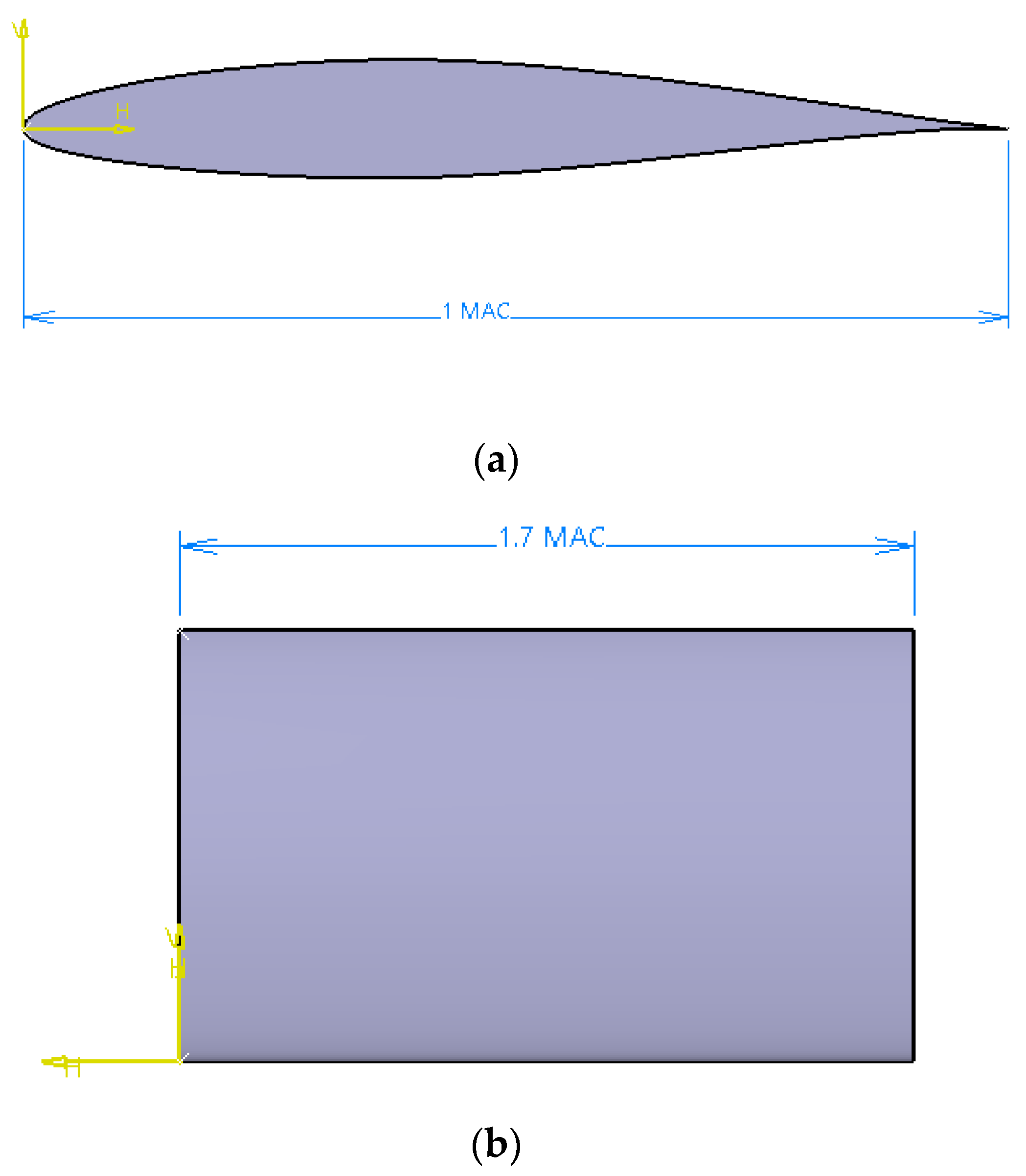
As mentioned in the previous section, the wing design was based on an NACA 641-212 airfoil. A thorough perspective of the designed wing section is illustrated in
Figure 1. The dimensions of the wing are expressed in units of the mean aerodynamic chord (MAC). As also mentioned in the previous section, the mean aerodynamic chord of the downscaled model was 0.1 m, while that for the original model was 0.43 m.
At this point, the reasons for selecting the downscaled model are analyzed. The main limiting factors are as follows:
- (a)
The maximum operating airflow speed produced by the wind tunnel drive motor is 33 m/s. It was selected to operate at 90% of its maximum capability, i.e.,
- (b)
The cross-section of the wind tunnel has dimensions 0.65 m × 0.65 m.
- (c)
The wingspan must not exceed 30% of the tunnel cross-section in length, to avoid the study suffering from blockage effects.
- (d)
The main objective was to maintain a constant Reynolds number both in the experiment and in the numerical simulations.
- (e)
The aspect ratio (AR) of the wing should remain constant for all models. For rectangle wings like our study’s,
Taking into consideration that the airflow velocity for the numerical simulations of the original size model was set to 7 m/s and combined with the limiting factors in Equations (5)–(8), the chord of the downscaled model was calculated to be 0.1 m and the downscaling factor was calculated to be 23%.
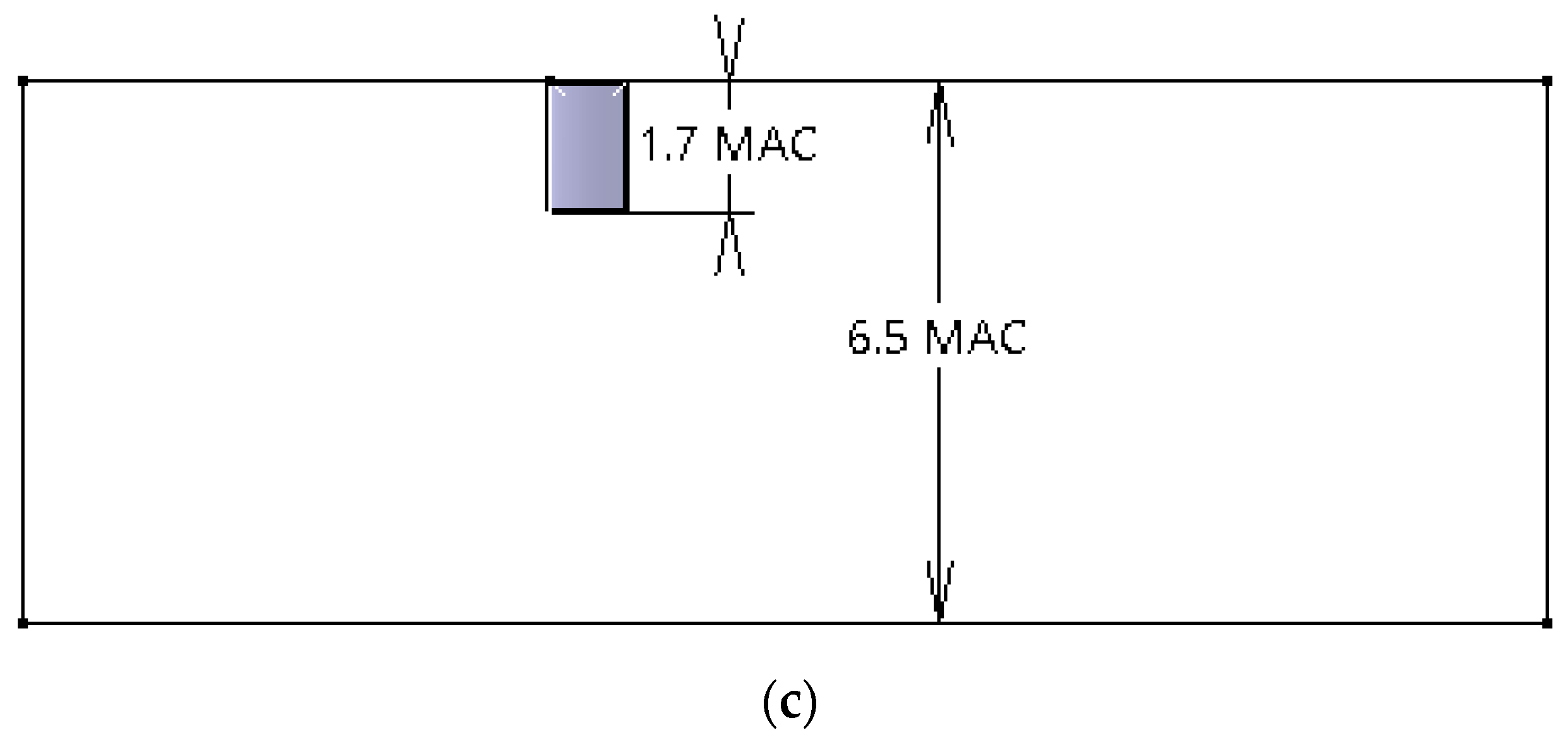
After completing the CAD design of the wing, the study utilized the commercial CFD code of Ansys Fluent for the execution of the numerical simulations. A three-dimensional domain, as shown in
Figure 2 and
Figure 3a, was created, containing the designed wing, and the RANS equations were solved. The dimensions of the domain are also expressed in units of the mean aerodynamic chord (MAC), and there is absolute agreement between the sizes of the simulation domain and the wind-tunnel measurement chamber where the wing model was mounted and tested. As shown in
Figure 2, the front and backward surface of the domain consisted of a square with dimensions 6.5 MAC × 6.5 MAC, while all four side surfaces consisted of a parallelogram with dimensions 20 MAC × 6.5 MAC. The wing, both in the computational domain and the wind-tunnel measurement chamber, was located as shown in both figures.
In order for the simulation to produce meaningful results, it was important to ensure that the geometry of the flow domain faithfully represents the experimental arrangement. Hence, for the analysis of this specific geometry, a type “H” computational domain was used. As shown in
Figure 3b, the computational domain became more finite moving from the external surface of domain toward the surface of the wing section. The size of the first cell of the meshed domain over the wing section was equal to 1.96 × 10
−5 m, in order to reach the boundary layer of the wing and to ensure that y
+ < 1.
The computational domain consisted of a fully structured mesh grid, where the region was divided into hexahedra, and it was constructed with the help of ICEM [
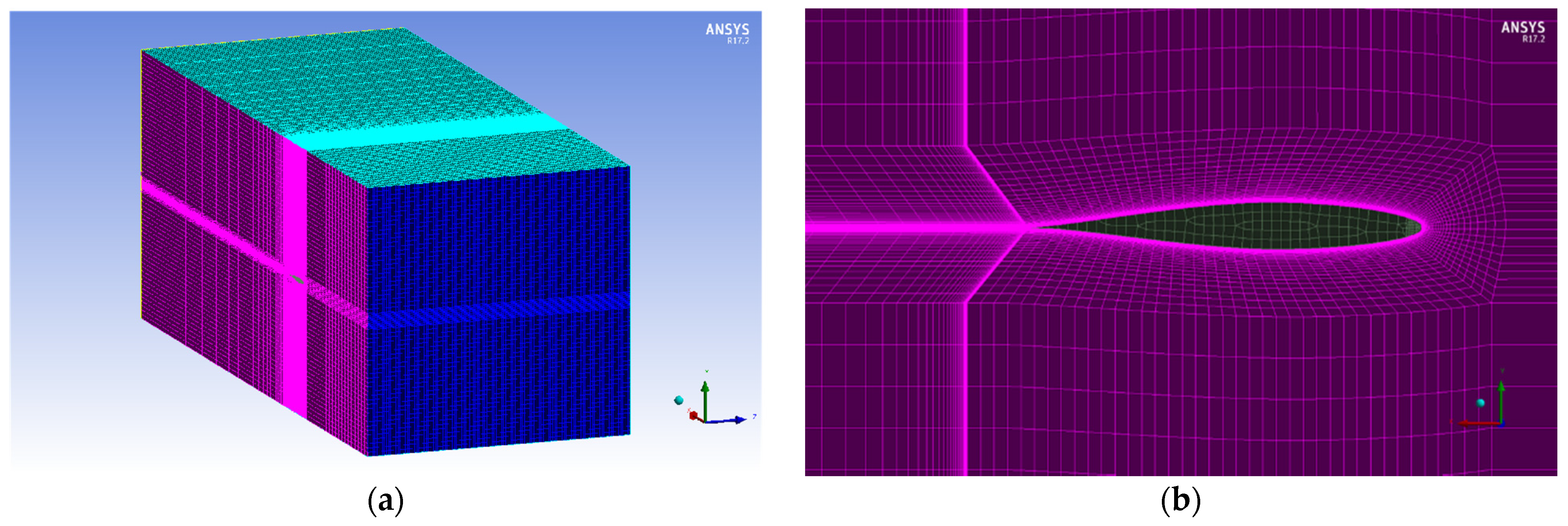
9]. A mesh independence study of the number of elements constituting the computational domain is one of the main stages of CFD analysis. In order to identify the minimum mesh density to ensure that the solution is independent of the mesh resolution, a mesh sensitivity analysis was carried out in the construction and analysis of the CFD model. The variation of drag and lift coefficient over the wing section at zero angle of attack is presented in the
Figure 4. The mesh study indicated that a computational domain of 4,800,000 elements for the original model and 1,350,000 elements for the downscaled model had accurate results.
After the generation of meshes, the study continued with the preparation for the numerical simulation, defining the turbulence model, the boundary conditions, and the numerical schemes to be utilized. As mentioned earlier in this study, the selected model for all cases of numerical simulations was Spalart–Allmaras, due to its suitability for aerospace applications involving wall-bounded flows and its good results for simple attached flows and slow separation locations.
For the simulations of the single-phase flow, the solver utilized in Fluent code was the pressure-based solver, considering a time-steady airflow, since the flow field conditions can be considered time-independent. The pressure-based coupled algorithm was used in order to enable a full pressure–velocity coupling. The second-order upwind scheme decreases the numerical discretization error; thus, from the start of the calculation, it was used for the spatial discretization due to the need for more accurate results for the final comparison with the experimental results and because of the implementation of two different mesh grids. The convergence criterion was set to a class of 1.0 × 10⁻⁶. As reference temperature, T = 284.18 K was considered; hence, the air density was set to ρ = 1.1561 kg/m3, and the dynamic viscosity was set to μ = 1.7701 × 10⁻⁵ kg/(ms), while the inlet velocity magnitude was set to 7 m/s and 30 m/s for the original and scaled models, respectively.
For the simulation of the discrete second phase, DPM was chosen with wall–film boundary conditions on the wing for the water droplets, to more realistically simulate the droplets’ behavior after the impact on the wing [
10,
11,
12]. The four walls of the domain were characterized as symmetrical at the boundary conditions, and the droplets were set to escape upon reaching them after collision with the wing.
The discrete phase was considered unsteady and set to interact with the continuous phase and be subject to gravitational forces. Two-way turbulence coupling was implemented, since we wanted to examine not only the particles’ behavior under the influence of continuum phase, but also the interaction between them and the changes in turbulent quantities due to particle damping and turbulence eddies. The dispersed entities were modeled as mass-points characterized by a parameter representing their size.
The second-phase injection into the airflow was achieved via a spray surface normal to the airflow covering the upper half of the inlet section, in a timestep of 0.001 s. The diameter of droplets was set to 0.0005 m. The velocity parallel to the airflow was set to 7 m/s and 30 m/s for the original and downscaled models, respectively. The total flow rate was set such that LWC = 40 g/m3 for both numerical simulations.
3. Experimental Procedure
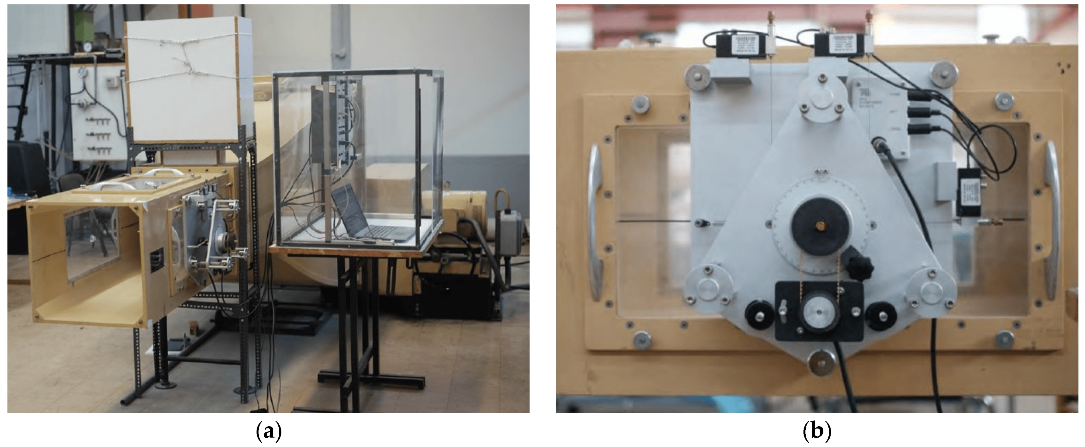
For the experimental study, the wind tunnel of the Fluid Mechanics and Fluid Applications Laboratory was used, in which the experimental model of the wing was placed, at a scale of 23% [
13]. The wind tunnel was the BLOWER TUNEL model made by Plint and Partners Ltd. Engineers in 1977. It is an open-type wind tunnel, i.e., the flow is discharged into the air immediately after the measurement chamber. This results in operation at pressure approaching atmospheric pressure, as well as easier access to the model. The measuring chamber has dimensions of 1.7 × 0.65 × 0.65 m, and it is equipped with three Plexiglas windows with removable frames, which facilitate access to the model and allow visual contact. To find the coefficients of lift and drag of the experimental model, the three-component AFA3 aerodynamic balance from TQ Education and Training Ltd. (London, UK) was used, as shown in
Figure 5; it is a device that measures two forces (lift and drag) and a moment (pitching moment). The display module was mounted onto the wind tunnel control and instrumentation frame and includes a digital display to directly show the lift, drag, and pitching moment. To fix the model to the aerodynamic balance, a shaft of 12 mm diameter and 220 mm length was used, placed in the socket of the balance retaining mechanism and secured by a special tightening bolt. In addition, the restraint mechanism was calibrated on the circumference and was free to rotate through 360°. Thus, we could precisely adjust the angle of attack of the model and immobilize it in the desired position with the help of the appropriate screw.
The aerodynamic balance is compatible with appropriate software, TecQuipment’s Versatile Data Acquisition System (VDAS), and it can quickly and conveniently connect to a frame-mounting interface unit. Using VDAS enables accurate real-time data capture, monitoring, display, calculation, and charting of all relevant parameters on the laboratory’s computer. This equipment is characterized by adequate precision since it can count forces with second-decimal precision, while its capacity is 100 N for lift, 50 N for drag, and 2.5 N·m for pitching moment. For every angle of attack examined, a set of force measurements were collected. Through the software, we set a timestep to record the value, which was 0.2 s. We chose to keep each angle of attack constant for at least 5 min during the operation of the wind tunnel in order to reduce the margin of error during the recording of the values. After a period of 5 min, more than 1500 values were recorded. These were collected for each angle of attack and first checked for possible outliers that could affect the mean value, before calculating the mean values of forces for every case.
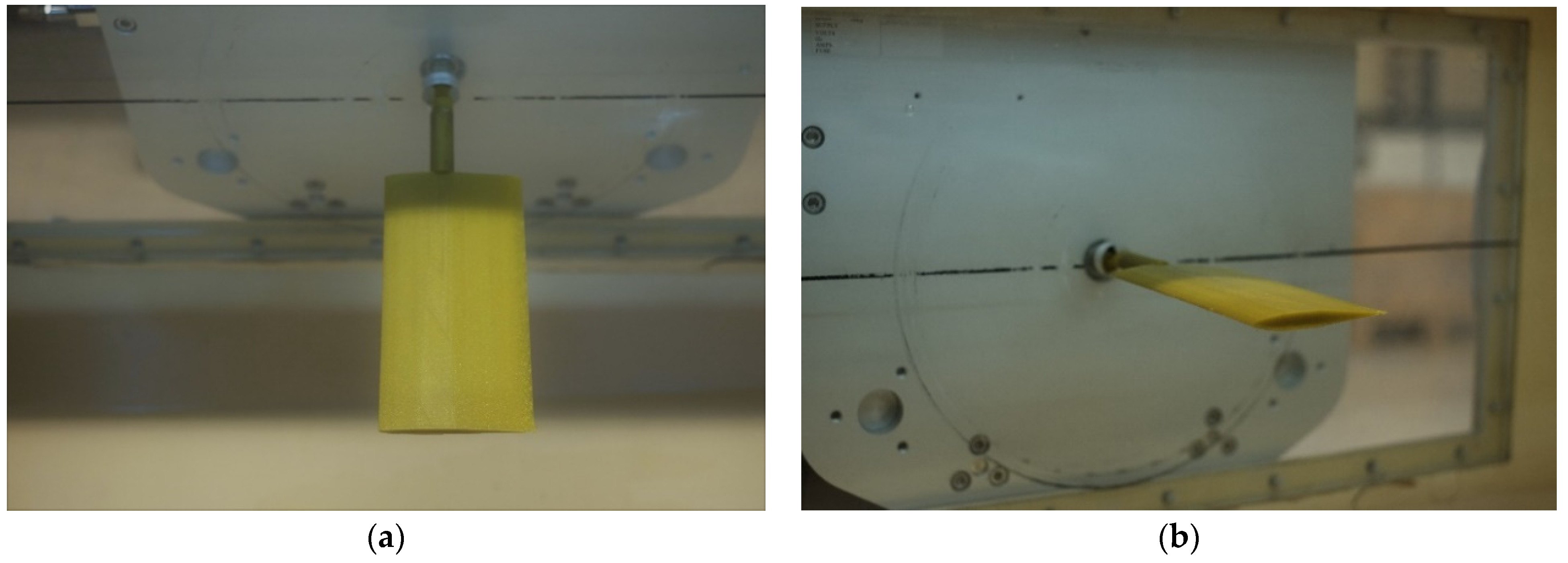
The experimental model used was a downscaled (23%) model of the original. The construction of the wing model was achieved with a generally recommended sequence of processes aimed at minimizing the construction material, which implies minimization of the weight and the cost. The experimental model was constructed using a 3D printer and then was subjected to a surface finishing treatment. The model was placed in the open wind tunnel and tested, as illustrated at
Figure 6 Lift and drag force were measured using the three-component aerodynamic balance, and the air velocity was determined using the inclined tube manometer to be 30 m/s.
4. Results
The numerical simulations were executed using the Spalart–Allmaras turbulence model. The results from those simulations were compared with the results from the wind-tunnel experiment for validation. Then, the results from the one-phase flow were compared with the results from the two-phase flow. The first step was to determine whether, for the same Reynolds number, there were significant differences in the results obtained by the simulations, between the two different model sizes. The second step was to investigate the effect of the second phase on the airflow and the aerodynamic behavior of the wing. This section is accordingly divided into two parts.
4.1. Validation of Initial Hypothesis
During the first stage of the research, numerical simulations were performed for the original wing and for the scaled model. Then, the corresponding experiment was performed in the wind tunnel, using the model identical to the scaled one, as mentioned in the previous section.
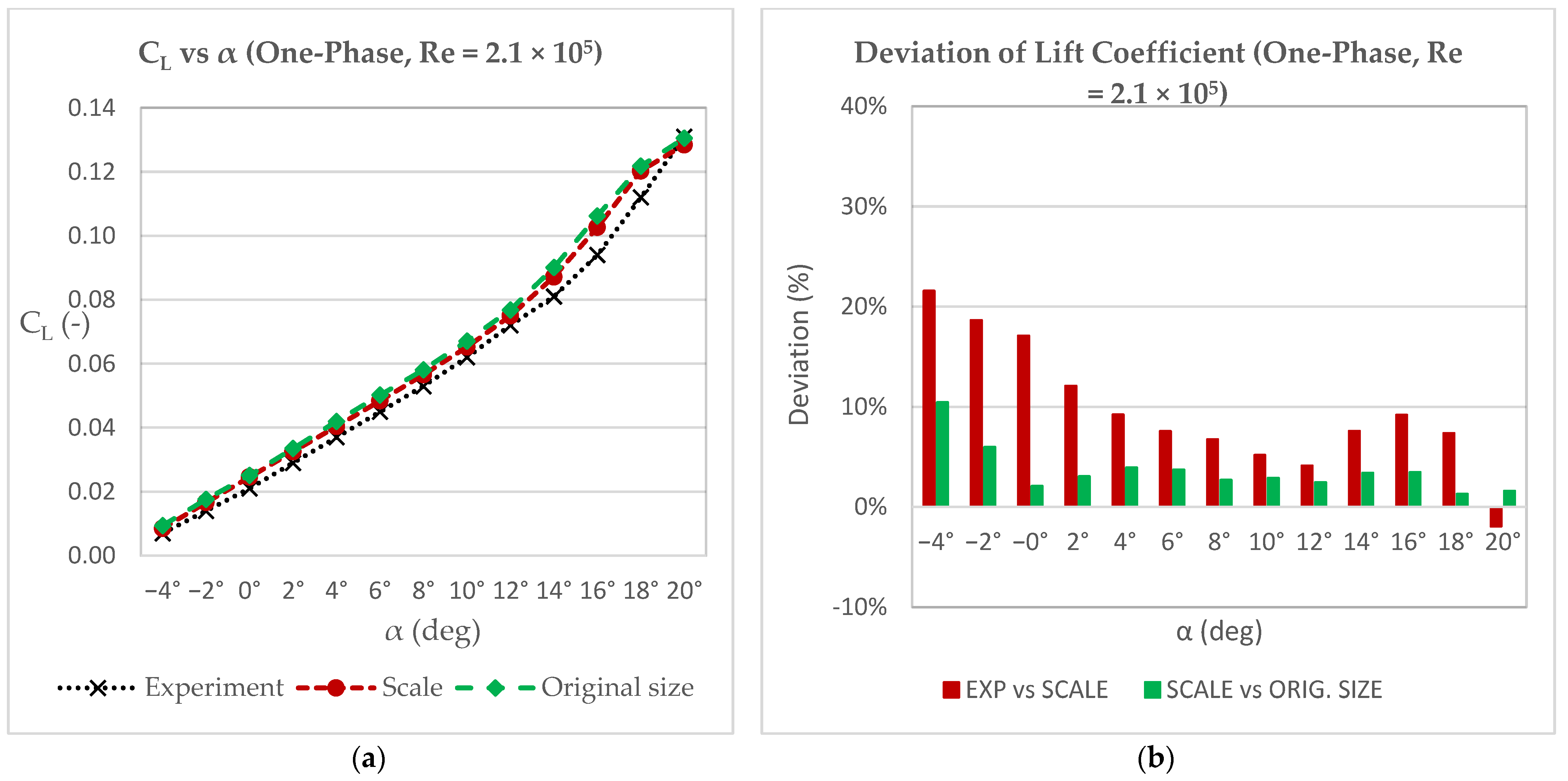
Figure 7a and
Figure 8a exhibit the two different cases of numerical simulations and the experimental simulation, with a Reynolds number of 2.1 × 10
5, using the Spalart–Allmaras turbulence model. The results demonstrated are those of the drag and lift coefficients.
By analyzing the results, it can be observed that, for the same Reynolds number, the values of the lift coefficient of the scaled model followed the corresponding values of the original model very closely, albeit slightly lower. Furthermore, we can observe the same behavior for the values of the lift coefficient obtained from the experiment with the same Reynolds number. According to a direct comparison of the values of the experiment with those of the scaled model, the wind-tunnel experiment yielded consistently lower values, but with relatively small deviations. This can be seen most clearly in
Figure 7b, where we can observe that, for angles from −4° to 2°, we had a deviation from 10% to 22%; however, from there to 20°, the difference between values was consistently below 10%. This led to an average deviation of 9.6%, thus validating the numerical simulation results of the downscaled model. The deviations between the actual and downscaled models are also given in
Figure 7b. It is clearly shown that the deviations were all below 5%, except at −4° and −2°, where they were 10.4% and 5.9%, resulting in an average deviation of 3.6%.
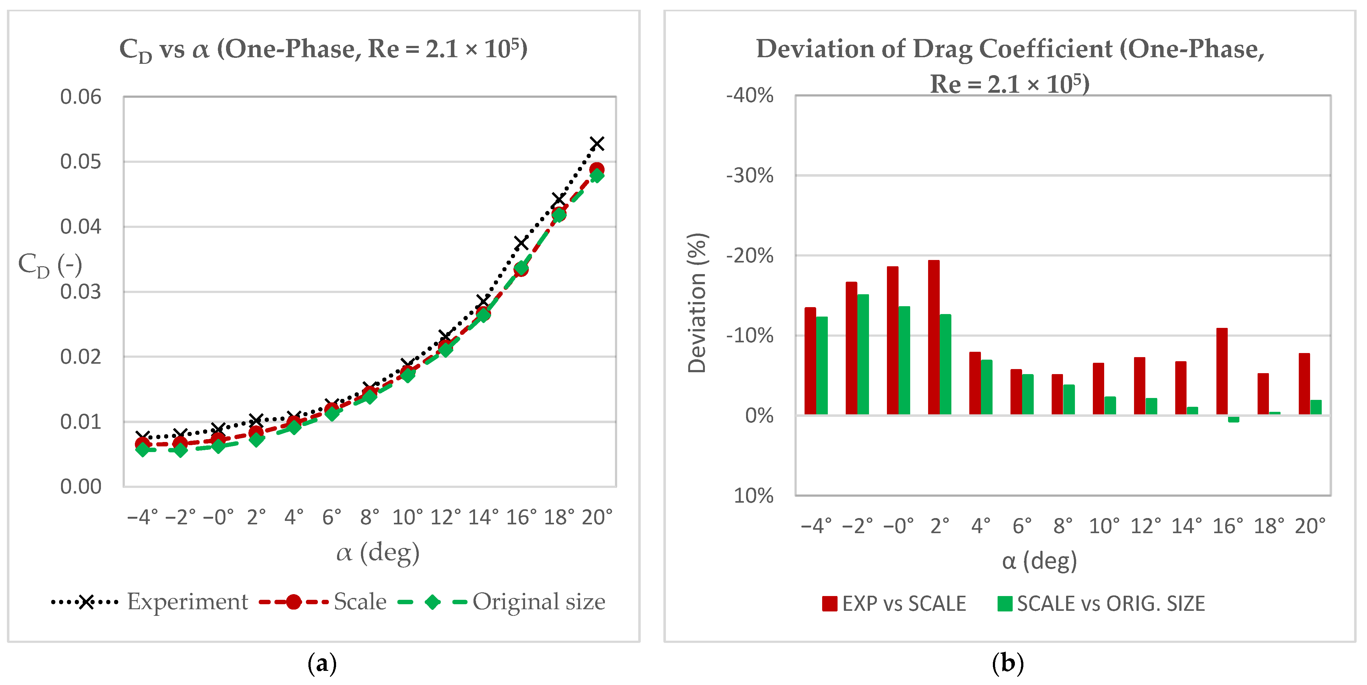
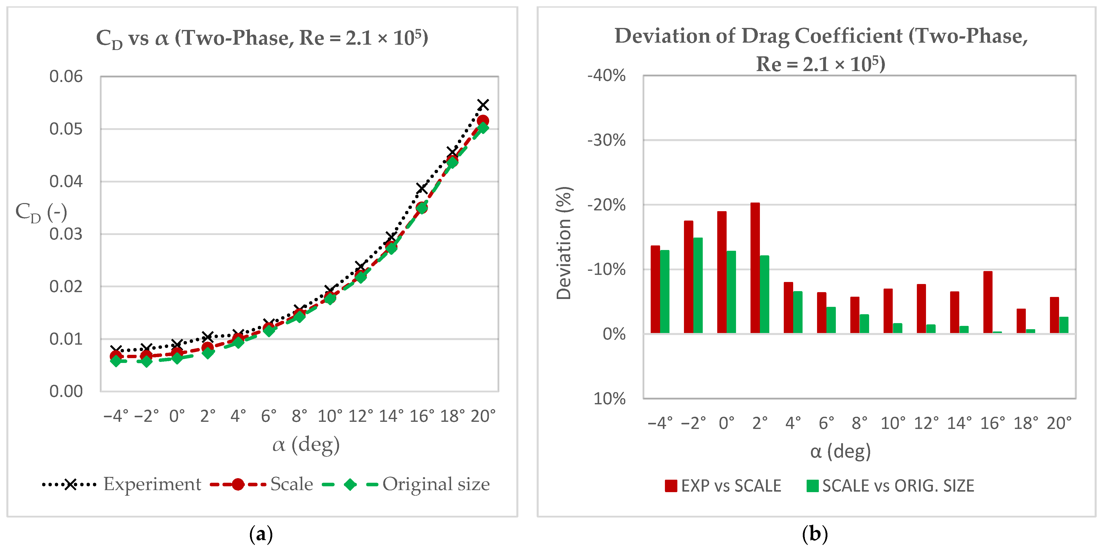
A similar trend occurred when studying the effects of the drag coefficient. As in the case of the lift coefficient, the results of the numerical simulations of the downscaled and original models were almost identical, with the original wing giving values marginally lower than the downscaled model over the whole range of the angles of attack. This can be seen in the
Figure 8b, where the average deviation was −5.8%. Moreover, the curve of the results from the experiment followed a similar trend to that of the scaled model. We can emphasize at this point that the experimental results presented a peculiarity with a divergence between 10% and 20% for angles from −4° to 2°, followed by very high convergence up to 16°. The average divergence of the results was on the order of 10%, marginally validating the numerical results of the scaled model.
After the completion of the simulations and the experiment in one-phase air flow, the simulations and the experiment were performed in two-phase flow. The numerical simulations were carried out using both the original wing and the scaled model, while the wind-tunnel experiment was carried out using the scaled model. The second phase was simulated with a droplet injection, maintaining LWC = 40 g/m3 in all three cases. The results obtained were discussed in terms of lift and drag coefficients and are presented in the comparative diagrams below. We can observe that the curves of both coefficients followed the same behavior as in the one-phase flow.
Again, we obtained almost identical values for the two simulation models; as shown in
Figure 9b and
Figure 10b, the lift coefficients of the two models had an average deviation of 3.7%, while the drag coefficients had an average deviation of −5.6%. Moreover, when comparing the values exported from the experiment with those from the numerical simulations of the downscaled model, the average deviation of the lift coefficients was 9.6%, while the average deviation of the drag coefficient values was −9.9%.
What is worth noting here is that the existence of the second phase negatively affected the aerodynamic behavior of the simulations and the experimental model, as discussed below. However, it did not cause any change in the trend of comparison between the simulations. In other words, the experimental model again yielded higher drag coefficient and lower lift coefficient values compared to the numerical simulations of the scaled model, over the full range of angles. Furthermore, the original model gave slightly lower drag coefficient and higher lift coefficient values compared to the scaled model.
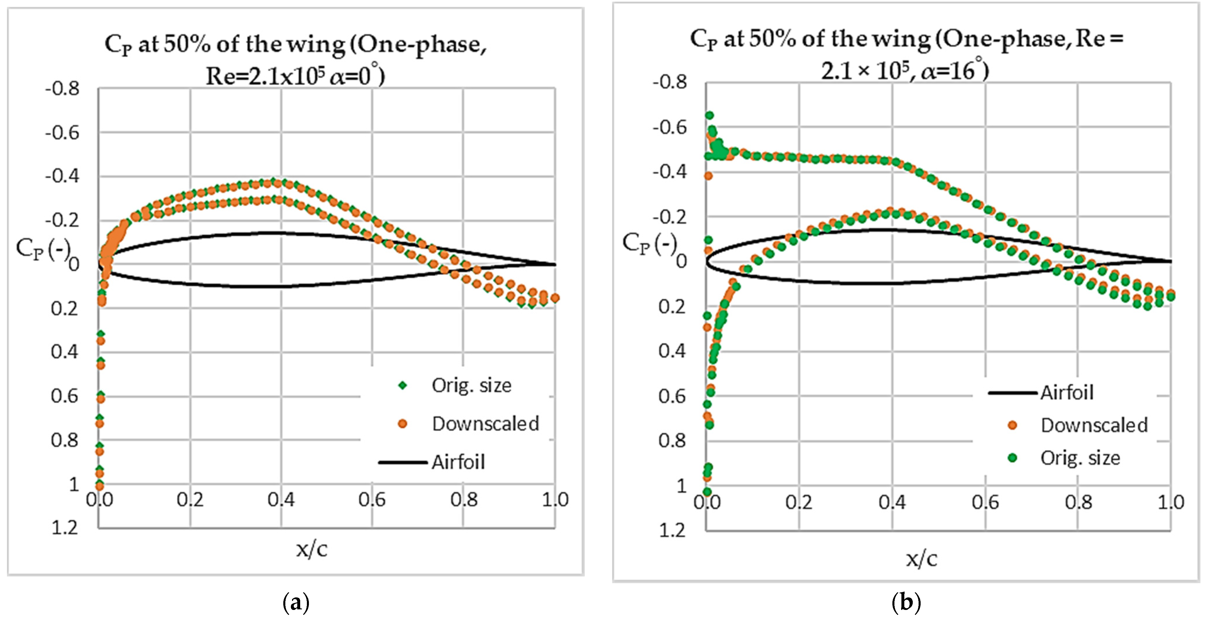
The diagrams in
Figure 11 show the distribution of the pressure coefficient over the entire surface of the airfoil. More specifically, an airfoil was selected at 50% of the wing, in both the scaled and the original models. This airfoil was studied at 0° and 16°. First of all, it should be emphasized that the pressure coefficients for both models at both angles of attack were almost identical over the entire length of the chord. It can also be observed that, as the angle of attack increased, the difference in C
p between the suction side and the pressure side increased for the same x/c. This had the effect of increasing the lift of the wing with an increase in the angle of attack.
Another conclusion that can be drawn is that, with increasing angle of attack, the airfoil of both models seemingly produced an increasing amount of lift from the leading edge. Furthermore, it is noteworthy that, at 0°, in both models, the lower surface also exhibited negative Cp, evidencing a downward force on the lower surface.
4.2. Impact of the Second Phase
The study continued with an evaluation of the influence of the second phase on the aerodynamic values of the wing. An overview of the effect is presented in the graphs of
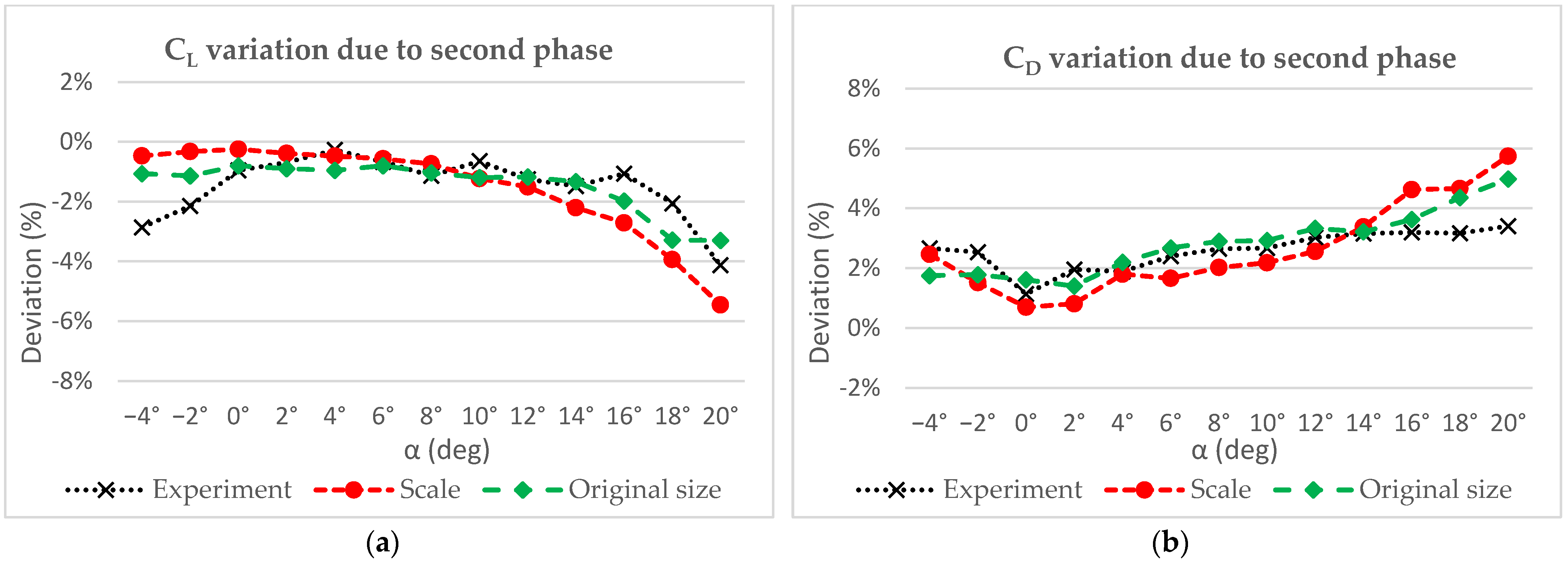
Figure 12, showing the percentage variation due to the second phase, over the whole range of angles of attack, for both the numerical simulations and the experimental procedure.
The presence of the second phase negatively affected the lift, in both the numerical simulations and the experiment. The reduction in lift was visible over the whole range of angles of attack, but did not remain constant. It can be observed that, in all three cases, the degradation was smaller at low angles of attack and increased with increasing angle. The percentage deterioration yielded values from −0.27% (4°) to −4.12% (20°) for the experimental procedure, with the average degradation being −1.49%. Correspondingly, for the numerical simulations of the downscaled model, values from −0.24% (0°) to −5.45% (20°) were obtained with a mean value of −1.56%, while, for the original model, the degradation ranged from −0.8% (0°) to −3.3% (20°) with a mean value of −1.46%.
Drag exhibited completely opposite behavior in the study of two-phase flow. The existence of the second phase was shown to increase drag. This increase presented its minimum value in the range 0° to 2° and increased with increasing angle of attack. The average increase in drag during the experiment was measured at 2.61%. For the numerical simulations, it was measured at 2.63% and 2.83% for the scaled and original models, respectively.
In
Table 1, L/D degradation is presented for both the numerical simulations and the experiment conducted in the subsonic wind tunnel. The general tendency shown is a decline in the aerodynamic efficiency due to the presence of the second phase. There is very good agreement among the three cases concerning the mean deviation of the aerodynamic efficiency, presenting values of −3.98%, −4.03%, and −4.15% for the experiment and the simulations of scaled and original models, respectively. This means that the wing experienced 4% loss, on average, of its aerodynamic efficiency due to the existence of the second phase.
The highest percentage degradation for all three cases appeared at 20° angle of attack, while the lowest values were obtained at 0° and 2°. What needs to be mentioned here is that, from −4° to 0° and 2°, the percentage deviation decreased, whereas the general tendency from 2° until 20° was an increase, for both the numerical simulations and the experiment.
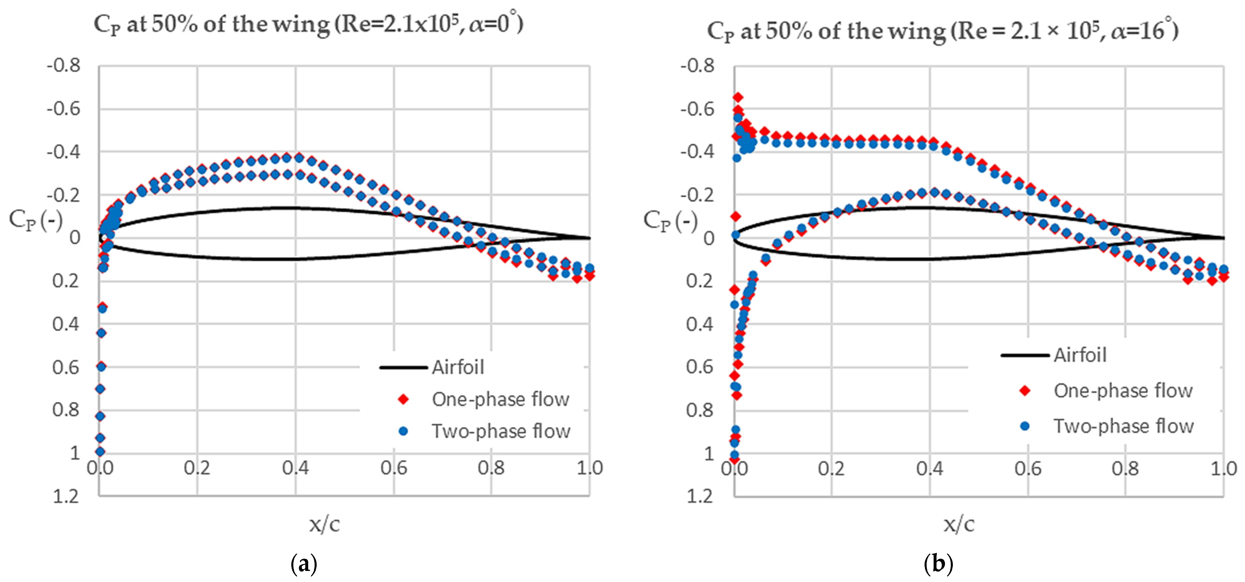
The presence of water droplets was proven, in the previous section, to negatively affect the aerodynamic behaviour of the wing. With a more thorough view of the pressure coefficient distribution graphs in
Figure 13, we can notice that the presence of the second phase resulted in the appearance of an adverse pressure gradient region slightly earlier than in the one-phase flow, at x/c ≈ 0.4 for both angles of attack.
The reduction in lift due to the second phase is also demonstrated in
Figure 13, where the enclosed region of pressure coefficients of two-phase flow was reduced compared to the corresponding region of one-phase flow. This phenomenon is even more intense in
Figure 13b, where the lift coefficient percentage was further reduced with increasing angle of attack due to the second phase.
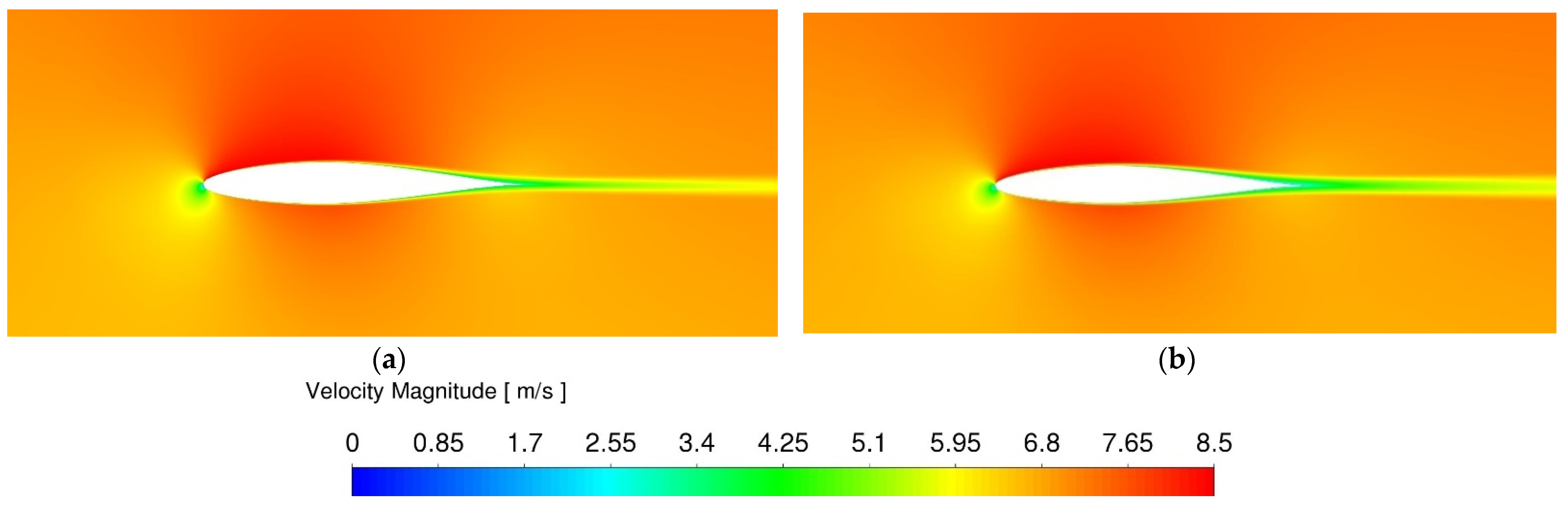
As shown in
Figure 14, the accelerating flow at the suction side of the wing seemingly obtained its maximum velocity at nearly 40% of the chord, and then the flow decelerated. The velocity magnitude contour, received from the two-phase flow, proves that the existence of the second phase was responsible for the formation of a thicker wake region compared to the one-phase flow.
Furthermore, on both the suction and the pressure sides of the wing during the two-phase flow, the deceleration of flow appeared to start earlier. Thus, the pressure difference between the upper and lower surface declined for the two-phase flow when compared to the one-phase flow. This led to the lift and the lift-to-drag ratio decreasing with the existence of the second phase.
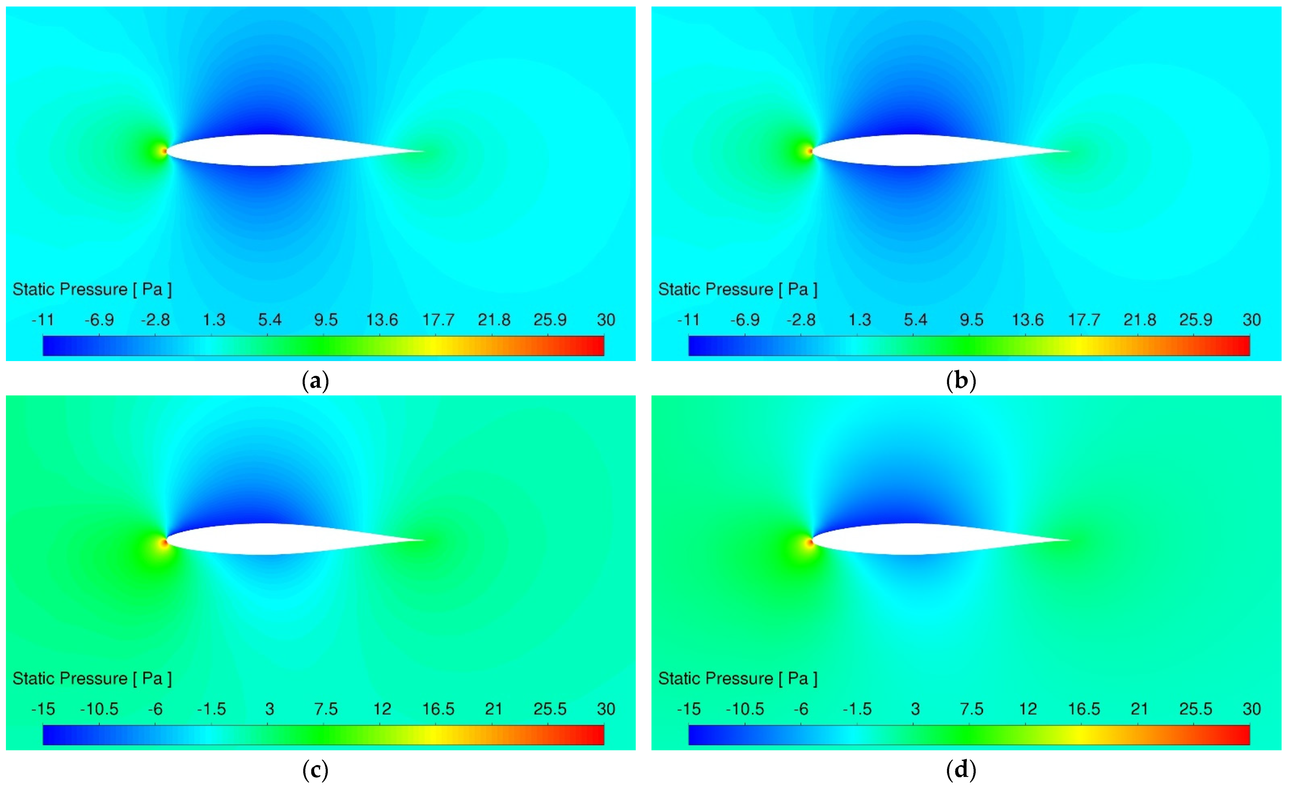
The contour of static pressure, in
Figure 15, exhibited an expected behavior, with minimum static pressure located over the section of the maximum curvature of the wing, whereas the highest pressure could be found on the leading edge. When the angle of attack increased, the pressure on the upper surface of the wing was significantly reduced, thus increasing the pressure differential between the upper and lower surface of the wing, leading to an increase in lift. This phenomenon occurred in both single-phase and two-phase flow. What needs to be mentioned is that the stagnation point moved from the upper surface of the leading edge to the lower surface with the increase in angle of attack.
It can be noticed that the pressure difference between the upper and lower surface declined slightly for the two-phase flow compared to the one-phase flow. This led to the lift and the lift-to-drag ratio decreasing with the existence of the second phase.
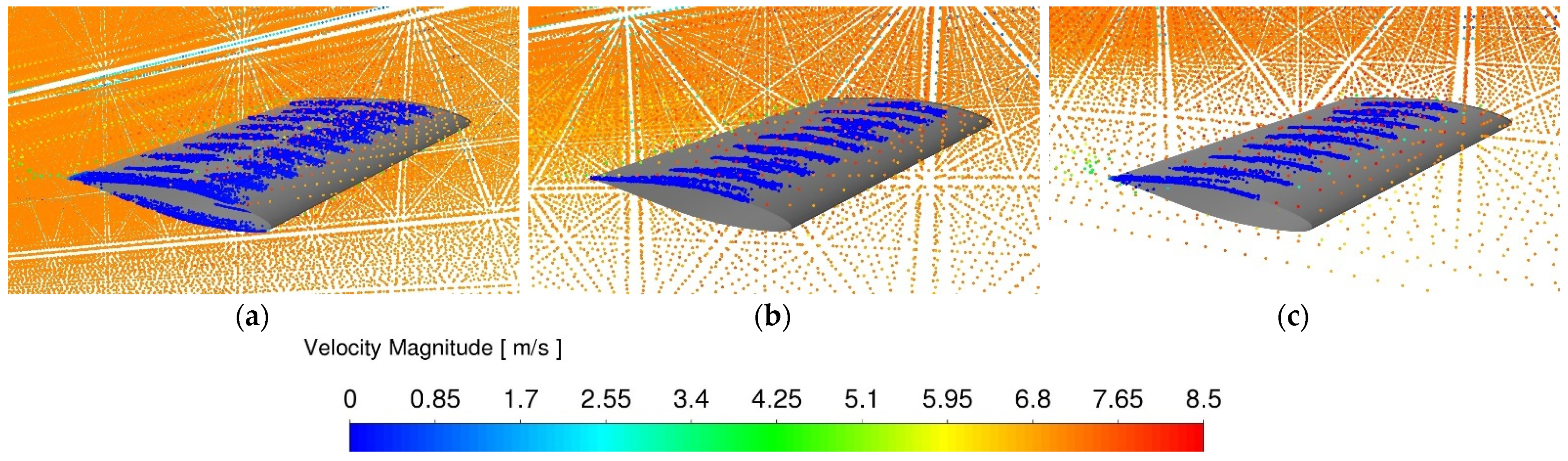
Lastly, the distribution of water particles around the wing can be observed in
Figure 16. Ιt should be noted that the color scale of the water droplets indicates the velocity magnitude of the water droplets. A thin layer of water, known as a water film, formed around the surface of the wing.
In addition, the water film was observed to break up into “streams” which flowed toward the trailing edge. The percentage of droplets breaking up depended on the diameter of the particles, as well as the angle of attack. Lastly, the water film showed a maximum thickness at one-third of the chord of the wing, where the maximum thickness of this film was found. According to the figures below, the computational results revealed water droplets breaking up into areas of increased pressure around the wing, while they formed these streams at regions with lower static pressure. When the droplets impinged with high velocity on the leading edge of the downscaled wing, a cloud of particles was created. An equally interesting point is that, with the increase in angle of attack, the width of the above-referred flow streams was reduced along the wingspan.
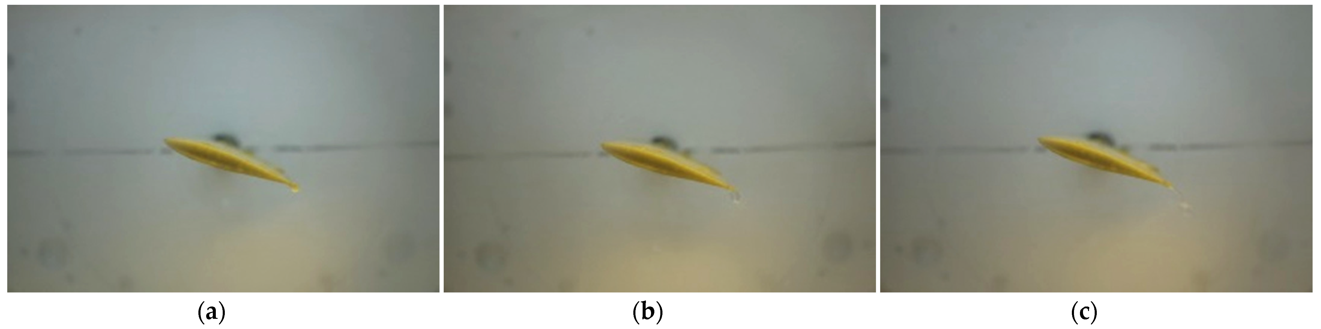
In
Figure 17, a water film can be observed to form on the upper surface of the wing during the two-phase flow experiment in the subsonic wind tunnel.
The wing was at 16° angle of attack during the process of acquiring the aerodynamic values, and we can observe how the water film formed and how the water droplets detached from the wing at the trailing edge.
5. Discussion and Conclusions
In this study, the design of a rectangular wing, based on an NACA 641-212 airfoil, was carried out with two different sizes of chord, 0.1 m (downscaled model) and 0.43 m (original model), and a constant aspect ratio 1.7. The aim of the research was to investigate whether a downscaled model simulation could offer us reliable results with less cost in terms of valuable computational resources and time.
The first stage involved the study of the wings’ aerodynamic behavior in the commercial Ansys Fluent simulation code at speed under Reynolds Number = 210,000 and at various angles of attack in both one-phase airflow and two-phase air–water flow. The results of the downscaled model were then compared to the results of the original wing model. Then, in a subsonic wind tunnel, an experiment was performed at boundary conditions identical to the numerical simulations, in both one-phase and two-phase flow. The numerical results were compared with the experimental ones for validation of the initial hypothesis.
The results of the downscaled model simulation compared to the experimental ones, showed an average deviation of 9.6% for the lift coefficient and 10% for the drag coefficient in the one-phase flow and of 9.6% for the lift coefficient and 9.9% for the drag coefficient in the two-phase flow. These results can be considered to validate the numerical simulations of the downscaled model. Furthermore, the average deviations between the numerical simulations of the two coefficients were measured at 5.9% or lower. Taking all these results into consideration, the feasibility of a downscaled model for simulating the aerodynamic behavior of a wing section, thus saving time, energy, and computational resources, can be verified. Considering tolerance for an average error of at most 10%, an early analysis of an aerodynamic case can be performed using a downscaled model, with high precision and reliable results. In particular, for two-phase flow simulations which are broadly known to require more time, energy, and resources, the benefits of simulating a downscaled model are even higher.
The second part of the study consisted of a comparison of the results between one-phase flow of air and two-phase flow of air–water. The results showed that the presence of water droplets in the flow resulted in a degradation of the aerodynamic performance of the wing at an average rate of about 4%, for both the numerical simulations and the experimental study. The differences in static pressure distribution around the wing between one-phase and two-phase flow demonstrated this aerodynamic decline. The differences in pressure coefficient distribution proved the deterioration of the lift and the lift-to-drag ratio due to the existence of the second phase. It is worth mentioning that this degradation was lower at low angles of attack, intensifying with increasing angle of attack.
Two triggering points should be discussed at this stage. The first is the uncertainty of the wind-tunnel measurements and their precision regarding the results for the lift and drag coefficients. As also expressed in
Section 2, the aerodynamic balance can record forces with second-decimal precision. In our case, the lift force, for incidence angles close to zero, varied in a range between 0.10 N and 0.40 N. The low nature of these values, an order of magnitude below or close to 1 N, raises questions of precision. Furthermore, the deviations in the measured lift between single-phase and two-phase flow are on the order of 0.01 N, i.e., at the limit of the maximum possible accuracy of the aerodynamic balance, thus exacerbating these concerns. In addition, the vibrations caused from the wind-tunnel motor operation seemingly caused fluctuations during the measures. Restricted to the supplied equipment, the best possible way to tackle all these uncertainties was to first thoroughly calibrate the aerodynamic balance prior to the experiment. During the experiment, 1500 values were recorded for each angle of attack; then, after the elimination of possible outliers, the mean value of force was counted. However, we recommend conducting the same experiment in a wind tunnel with higher precision.
The second point which may raise concern regards the fact that, over 16° angle of attack, the lift coefficient continued to increase. According to NASA Technical Memorandum NASA-TM-X-3293 [
14], the lift coefficient of the NACA 641-212 airfoil seems to stall at a critical angle of 16°. However, the rectangular wing of our study did not appear to reach the stall angle until 20°. It is widely known that a three-dimensional wing allows air to flow over the wingtip into the low-pressure zone over the wing, thus reducing the overall pressure differential and reducing overall lift. This explains the stall at a higher angle of attack, compared to the two-dimensional airfoil, because the additional airflow over the wing surface “energizes” the air. Flow separation happens when the kinetic energy is equal to the pressure differential that the airstream flows into; therefore, if the kinetic energy can be increased, the tendency of the airstream to separate can be decreased. This briefly explains why, in our simulations, the lift coefficient continued to increase at angles higher than 16°. What may be suggested for future research is to perform simulations at angles of attack higher than 20°, in order to reach the stall angle of the wing section.


 ,
, 


