Computational Fluid Dynamics Study of Wing in Air Flow and Air–Solid Flow Using Three Different Meshing Techniques and Comparison with Experimental Results in Wind Tunnel

Abstract

The main purpose of this work is to simulate the flow of air and solid particles over a wildfire and to investigate the single and multiphase flow over the surface of a custom-designed wing with an Eppler-420 airfoil including an appendant custom-designed blended winglet. The wing is the result of a conceptual and preliminary design of a small-scale unmanned aerial vehicle (UAV) designed to assist in firefighting. The fire embers will be simulated in the Ansys Fluent commercial code as solid particles injected in the continuous phase, in an Euler–Lagrange approach. Primarily studied were the response of the model in air and air–solid flows, as well as the impact on aerodynamic efficiency due to the existence of the second phase. Moreover, the effects of unstructured, structured and mosaic poly-hexcore meshes are investigated and compared. The computational fluid dynamics (CFD) simulations, were implemented using a pressure-based solver, spatial discretization was conducted with a second-order upwind scheme, and the k-omega SST (k-ω SST) turbulence model was applied. Meanwhile, the two-phase flow was simulated using the Discrete Phase Model with reflect boundary condition on the surface of the wing and two-way coupling between continuous and discrete phase. To validate the results, experiments were conducted in a subsonic wind tunnel using a 3D printed model of the wing. The results show good agreement between simulations and experiments, with the structured mesh coming closer to reality, followed by the mosaic and unstructured meshes, respectively. Finally, a reduction in the aerodynamic efficiency of the wing section is observed, due to the presence of solid particles.

1. Introduction

Since ancient times, mankind has been confronted with the phenomenon of forest fires and has been trying to find ways to successfully combat them. In the last century, with the emergence and rapid development of aviation, man has used flying machines in the battle against this destructive phenomenon. An entire branch of aeronautics was and still is engaged in the research and development of fire-fighting aircraft, aiming to be more efficient and safer for their operators. This is the field this study is investigating.

In recent decades, the study of external two-phase flow around aerodynamic surfaces has intensified. However, the majority of research is focused on the study of air–water two-phase flow, while there is less study volume and corresponding results and data of air–solid two-phase flow.

Douvi et al. [1] studied the effects of air–sand flow over NACA 0012 airfoil at Reynolds (Re) 1.76 × 10⁶ and detected a degradation in lift coefficient and an increase in drag coefficient due to the presence of the second phase, for a wide range of angles of attack. At the same time, the solid particles appear to concentrate, for lower angles of attack, mainly at the upper surface and in the region between the leading edge and the middle of lower surface. When the angle of attack increases, the solid particles appear to concentrate on a smaller region of the airfoil. Similarly, Salem et al. [2] conducted a computational study on the NACA 63-215 airfoil using the k-ω SST turbulence model to investigate the impact of sand particles to its aerodynamic efficiency. An increase in drag coefficient due to increased surface roughness and a decline in lift coefficient due to premature separation and transition to turbulence were observed, a phenomenon caused by the dust accumulation near the leading edge. Zidane et al. [3] investigated the behaviour of the NACA 63-415 airfoil under two-phase flow of air–sand and concluded that there is an increase in degradation of the lift coefficient with the increase in sand particles’ flow rate. Ren and Ou [4] outlined that the roughness height produced by the solid particles’ concentration on a NACA 63-340 Airfoil influences lift and drag coefficients.

In the current study, a preliminary design of a small-scale firefighting aircraft has been performed. This has resulted in the initial design of a wing with special characteristics for the specific flight requirements. The study consists of three stages.

The first objective is to study this wing in single-phase flow, to derive its basic aerodynamic quantities and behaviour. Subsequently, an experiment will be performed in a subsonic flow wind tunnel to validate the results.

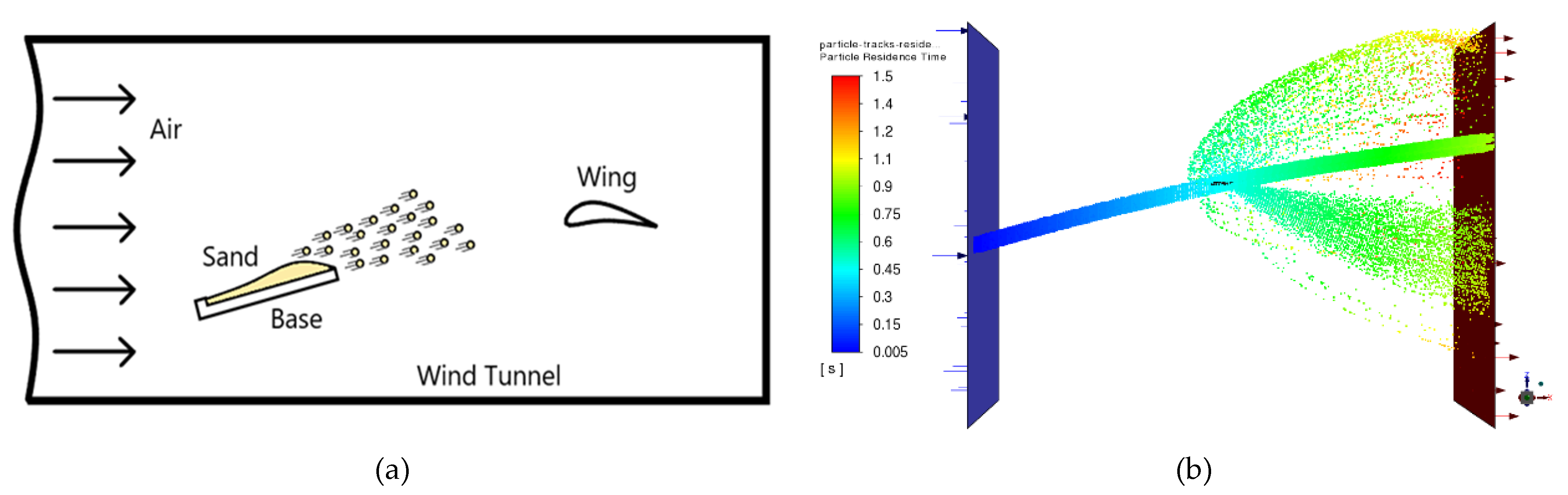
In the second stage of the study, the two-phase air solid flow will be investigated, aiming to simulate as best as possible the flight stage over a fire, in which small solid particles-products of combustion-rise. As an assumption, only the motion of the solid particles in the vertical axis will be studied, and not the fluid-thermal phenomena produced by combustion which may also influence the aerodynamic behaviour of the wing. The way the existence of a second solid phase affects the wing will be investigated and compared to single phase flow in the numerical simulation. The results will once more be validated by running an experiment in a subsonic wind tunnel. As flight over a forest fire could not be directly simulated by burning wood in the wind tunnel due to laboratory regulations, the solid particles will be simulated using medium sand, in accordance with ISO 14688-1:2002, spread on an inclined base. The experimental results will be compared with the results of the aforementioned two-phase flow numerical simulation, with the second phase also consisting of sand.

The third and final stage of the study regards a new two-phase flow numerical simulation, substituting sand with anthracite particles. The results will be compared and contrasted with the validated two-phase flow simulation using sand particles of stage two.

It must be underlined that the simulations will be performed with all three different meshing configurations. In the first case, an unstructured mesh will be used. In the second case, with the help of ICEM, a fully structured mesh will be used, whereas the third case will regard a mosaic poly-hexcore mesh. The results of all three cases will, in turn, be compared with the results of the wind tunnel experiments, to investigate which of the three meshing techniques leads to results closer to those of the experiments.

2. Numerical Methods and Simulation

Time-dependent solutions of the Navier–Stokes equations for high Reynolds-number turbulent flows in complex geometries, which set out to resolve all the way down to the smallest scales of the motions, are unlikely to be attainable for some time to come. Two alternative methods can be employed to render the Navier–Stokes equations tractable, so that the small-scale turbulent fluctuations do not have to be directly simulated: Reynolds-averaging (or ensemble-averaging) and filtering [5].

Both methods introduce additional terms in the governing equations that need to be modeled to achieve a “closure” for the unknowns. The Reynolds-averaged Navier–Stokes (RANS) equations govern the transport of the averaged flow quantities, with the whole range of the scales of turbulence being modeled. Therefore, the RANS-based modeling approach greatly reduces the required computational effort and resources and is widely adopted for practical engineering applications.

The k-ω turbulence model [6] is one of the most used models to capture the effect of turbulent flow conditions. It belongs to the Reynolds-averaged Navier–Stokes (RANS) family of turbulence models, where all the effects of turbulence are modeled. It is a two-equation model. That means that, in addition to the conservation equations, it solves two transport equations (PDEs), which account for the history effects such as convection and diffusion of turbulent energy. The two transported variables are turbulent kinetic energy (k), which determines the energy in turbulence, and specific turbulent dissipation rate (ω), which determines the rate of dissipation per unit of turbulent kinetic energy. The variable ω is also referred to as the scale of turbulence.

The standard k-ω model [5] is a low Re model, i.e., it can be used for flows with low Reynolds number, where the boundary layer is relatively thick, and the viscous sub-layer can be resolved. Thus, the standard k-ω model is best used for near-wall treatment. Other advantages include a superior performance for complex boundary layer flows under adverse pressure gradients and separations (e.g., external aerodynamics and turbomachinery). Furthermore, this model has also shown to predict excessive and early separations.

SST stands for shear stress transport. The SST formulation switches to a k-epsilon behaviour in the free-stream, which avoids the k-ω problem of being sensitive to the inlet free-stream turbulence properties. The k-ω SST model [7,8] provides a better prediction of flow separation than most RANS models and accounts for its good behaviour in adverse pressure gradients. It is able to account for the transport of the principal shear stress in adverse pressure gradient boundary layers [9]. It is the most used model in the industry, given its high accuracy to expense ratio.

The SST k-ω model has a similar form to the standard k-ω model:

$$\frac{\partial }{\partial t}\left(\rho k\right)+\frac{\partial }{\partial x_i}\left(\rho k{u}_i\right)=\frac{\partial }{\partial x_j}\left({\Gamma }_k\frac{\partial k}{\partial x_j}\right)+{\tilde{G}}_k-Y_k+S_K$$

(1)

where ${\tilde{G}}_k$ represents the generation of turbulence kinetic energy due to mean velocity gradients, ${\Gamma }_k$ represents the effective diffusivity of k, $Y_k$ represents the dissipation of k due to turbulence and $S_K$ is a user-defined term.

$$\frac{\partial }{\partial t}\left(\rho \omega \right)+\frac{\partial }{\partial x_i}\left(\rho \omega u_i\right)=\frac{\partial }{\partial x_j}\left({\Gamma }_{\omega }\frac{\partial \omega }{\partial x_j}\right)+G_{\omega }-Y_{\omega }+D_{\omega }+S_{\omega }$$

(2)

where $G_{\omega }$ represents the generation of $\omega$,${\Gamma }_{\omega }$ represents the effective diffusivity of $\omega$, $Y_{\omega }$ represents the dissipation of $\omega$ due to turbulence,$D_{\omega }$ represents the cross-diffusion term and $S_{\omega }$ is a user-defined term.

The numerical calculation of multiphase flow is accomplished with the Eulerian–Lagrangian approach. In Eulerian–Lagrangian approach, the fluid phase is treated as a continuum by solving the time-averaged Navier–Stokes equations, while the dispersed phase is solved by tracking a large number of solid particles, bubbles, or droplets through the calculated flow field. The dispersed phase can exchange momentum, mass, and energy with the fluid phase. In addition to solving transport equations for the continuous phase, a discrete second phase in a Lagrangian reference frame can be simulated.

This model is called Discrete Phase Model (DPM) and consists of spherical particles, which represent solid particles, droplets or bubbles dispersed in the continuous phase. The trajectories of these discrete phase entities are computed, as well as heat and mass transfer to/from them. The coupling between the phases and its impact on both the discrete phase trajectories and the continuous phase flow can be included. The trajectory of a discrete phase particle can be predicted by integrating the force balance on the particle, which is written in a Lagrangian reference frame. This force balance equates the particle inertia with the forces acting on the particle [5], and can be written (for the x direction in Cartesian coordinates) as

$$\frac{\mathrm{d}{u}_{\rho }}{\mathrm{d}t}=F_D\left(u-u_P\right)+\frac{g_x\left({\rho }_p-\rho \right)}{{\rho }_P}+F_x$$

(3)

where $F_x$ is an additional acceleration (force/unit particle mass) term, $F_D\left(u-u_P\right)$ is the drag force per unit particle mass and

$$F_D=\frac{18\mu }{{\rho }_p{d}_p^2}\frac{C_{D}R\mathrm{e}}{24}$$

(4)

Here, $u$ is the fluid phase velocity, $u_P$ is the particle velocity, μ is the molecular viscosity of the fluid, $\rho$ is the fluid density, ${\rho }_p$ is the density of the particle and ${\mathrm{d}}_p$ is the particle diameter. $R\mathrm{e}$ is the relative Reynolds number, which is defined as

$$R\mathrm{e}=\frac{\rho {\mathrm{d}}_P\left|u_P-u\right|}{\mu }$$

(5)

In the present simulation, both one-phase and two-phase flows were investigated with a free-stream velocity of Re = 65,000. The subsonic wind tunnel experiments were conducted at the same Reynolds Number. The results compared were the Coefficients of Lift, Drag and Pressure, and Aerodynamic Efficiency in each different case. The flow at six different angles of attack was simulated, to ensure safe results for a total study of the aerodynamic performance of the wing section.

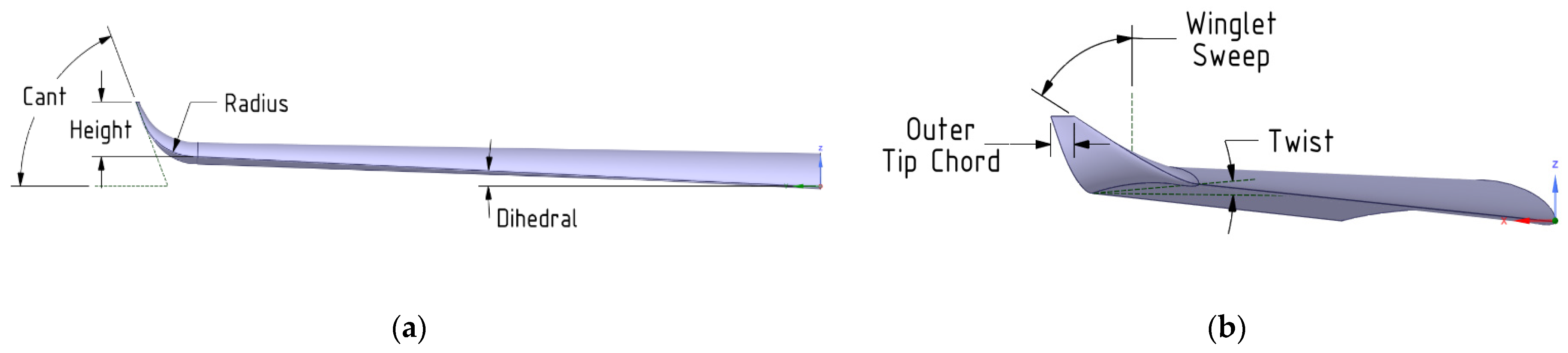
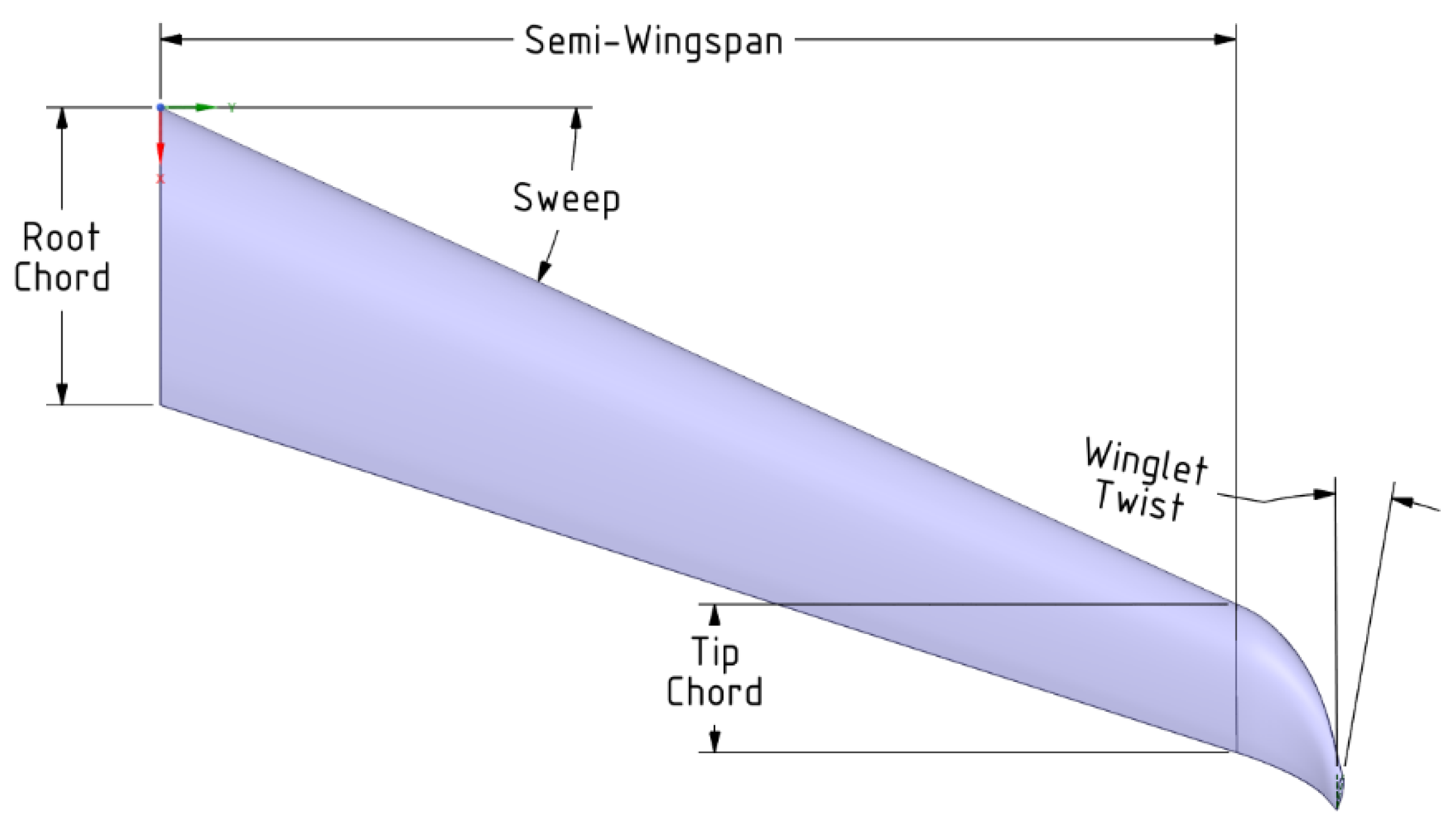
The wing section that was selected to be studied resulted from a preliminary study and conceptual design of a UAV. Thus, it is a custom-designed wing using computer-aided design (CAD) software from scratch, attempting to fulfil the flight requirements of the aircraft [10,11]. The main aerodynamic characteristics of the wing are that is based on the Eppler-420 airfoil, with a sweep angle of 25 degrees, a twist angle of 5 degrees and a dihedral angle of 2 degrees, while the wingtip has been replaced by a custom-designed blended winglet [12].

A thorough perspective of the designed wing section is illustrated in Figure 1 and Figure 2, while the values of the aerodynamic features are presented in

Table 1. Features of the designed wing.

Feature	Value
Airfoil	Eppler 420
Semi-wingspan	0.65 m
Root chord	0.18 m
Tip chord	0.09 m
Sweep angle	25°
Twist angle	5°
Dihedral Angle	2°

. As mentioned earlier, the blended winglet used is custom-designed to fulfil the wing’s conceptual design requirements, and the corresponding geometric features are presented in

Table 2. Features of the designed winglet.

Feature	Value
Cant angle	70°
Sweep angle	55°
Twist angle	10°
Height	0.06 m
Radius	0.06 m
Outer tip chord	0.02 m

.

It must be mentioned that for the execution of the experiments, the wing was not manufactured with conventional machining procedures. Due to its special geometric characteristics, it was decided to 3D-print the wing and then surface-finish it, to minimize skin friction drag and to simulate the real aluminum surface utilized in numerical simulations.

Following completion of the wing’s CAD design, the study involved utilization of the commercial CFD Ansys Fluent Code to execute the numerical simulations. A 3-dimensional domainwas created, in which the designed wing would be contained, and the RANS equations would be solved. As mentioned in the introduction, three different meshing configurations would be utilized to simulate the real conditions.

These configurations are the unstructured mesh with the segmentation of the grid in tetrahedra, the Mosaic poly-hexcore mesh, based on the connection of high-quality octree hexahedra in the bulk region and isotropic poly-prisms in the boundary layer with the Mosaic polyhedral elements, and finally the structured mesh with the region divided in hexahedra [13].

At this point, it is necessary to provide a special reference regarding the mosaic poly-hexcore mesh. The method in question is a relatively new ANSYS Mosaic Meshing technique, which uses high-quality hexahedral elements in the bulk region, keeps a high-quality layered poly-prism mesh in the boundary layer, and conformally connects these two meshes with general polyhedral elements. Since domain volume is generated with hexahedral elements for the same grid resolution, there is a total face count reduction. This methodology results in faster solve times, with a time reduction of 30–50% having been observed [14,15]. Additionally, Fluent meshing allows for parallel volume meshing on up to 256 cores, which, along with the lower overall mesh counts from Mosaic mesh, helps accelerate the meshing process. The Mosaic mesh of the present work uses the Poly-Hexcore method and consists of 2,607,133 cells, with a minimum orthogonal quality of 0.196808 and a maximum skewness of 0.803192. Having taken into consideration the inflation used by Gueraiche [16], and following trial and error, 15 inflation layers were used, with the last-ratio method. The first layer height was chosen to be 0.0015 mm, aiming to retain the value of y⁺ < 5.

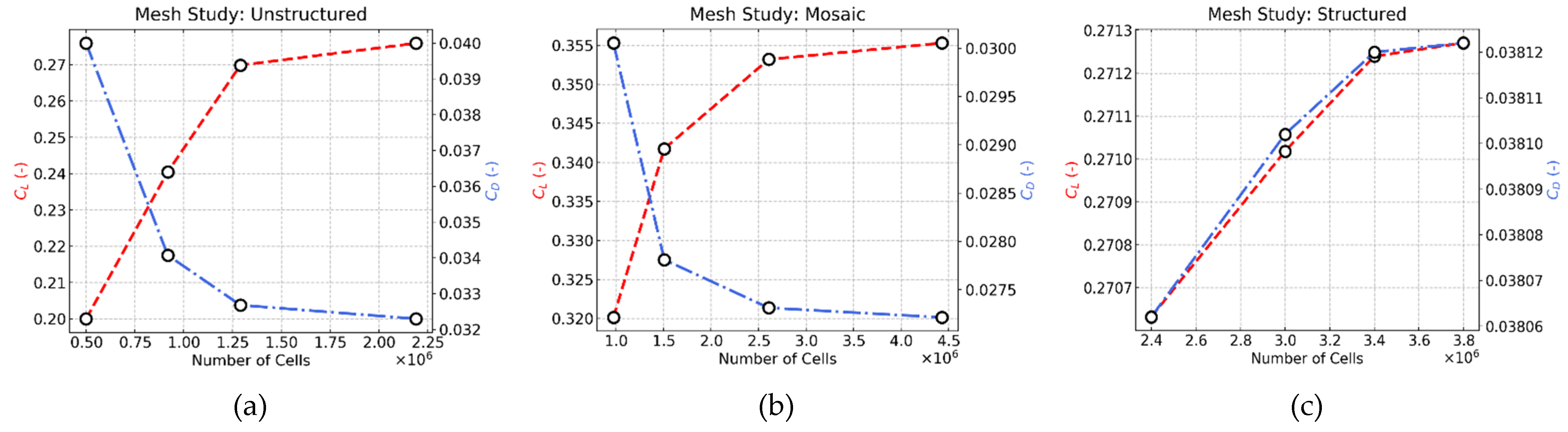
The selected meshes came as results of a mesh independence study, an essential step prior to the launch of numerical simulations, conducted for all three meshing configurations. The mesh independence study is paramount to this paper, serving the main objective of comparing aerodynamic behaviours and results from the three different meshes. The most appropriate number of cells in the computational mesh is found by increasing the number of cells until further increases do not significantly affect the results of the requested coefficients.

In Figure 3, it is observed that the unstructured grid with 1,290,802 cells, mosaic grid with 2,607,133 cells and the structured grid with 3,400,562 cells provide satisfactory solutions, independent of the number of cells. Therefore, these meshes are reliable and will be selected for use in the numerical simulations of the wing.

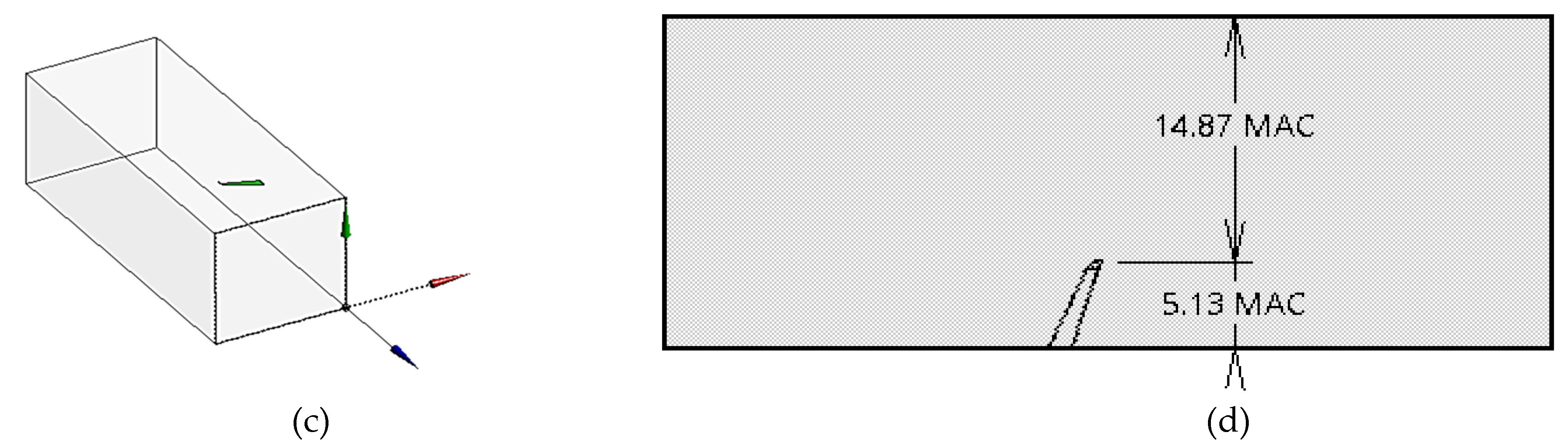
The computational domain was decided to be a rectangular parallelepiped. The main reason for selecting this shape was to fully simulate the layout of the wind tunnel’s measurement chamber and to ensure that the exact size ratios were maintained.

The dimensions of the domain are expressed in units of the mean aerodynamic chord (MAC), and there is absolute agreement between the sizes of the simulation domain and the wind tunnel measurement chamber where the wing model was mounted and tested. As seen in Figure 4, the frontal and backward surfaces of the domain consist of a square measuring 20 MAC × 20 MAC, while the remaining four side surfaces consist of a parallelogram measuring 50 MAC × 20 MAC. The wing, both in the computational domain and the wind tunnel measurement chamber, is located as shown in Figure 4.

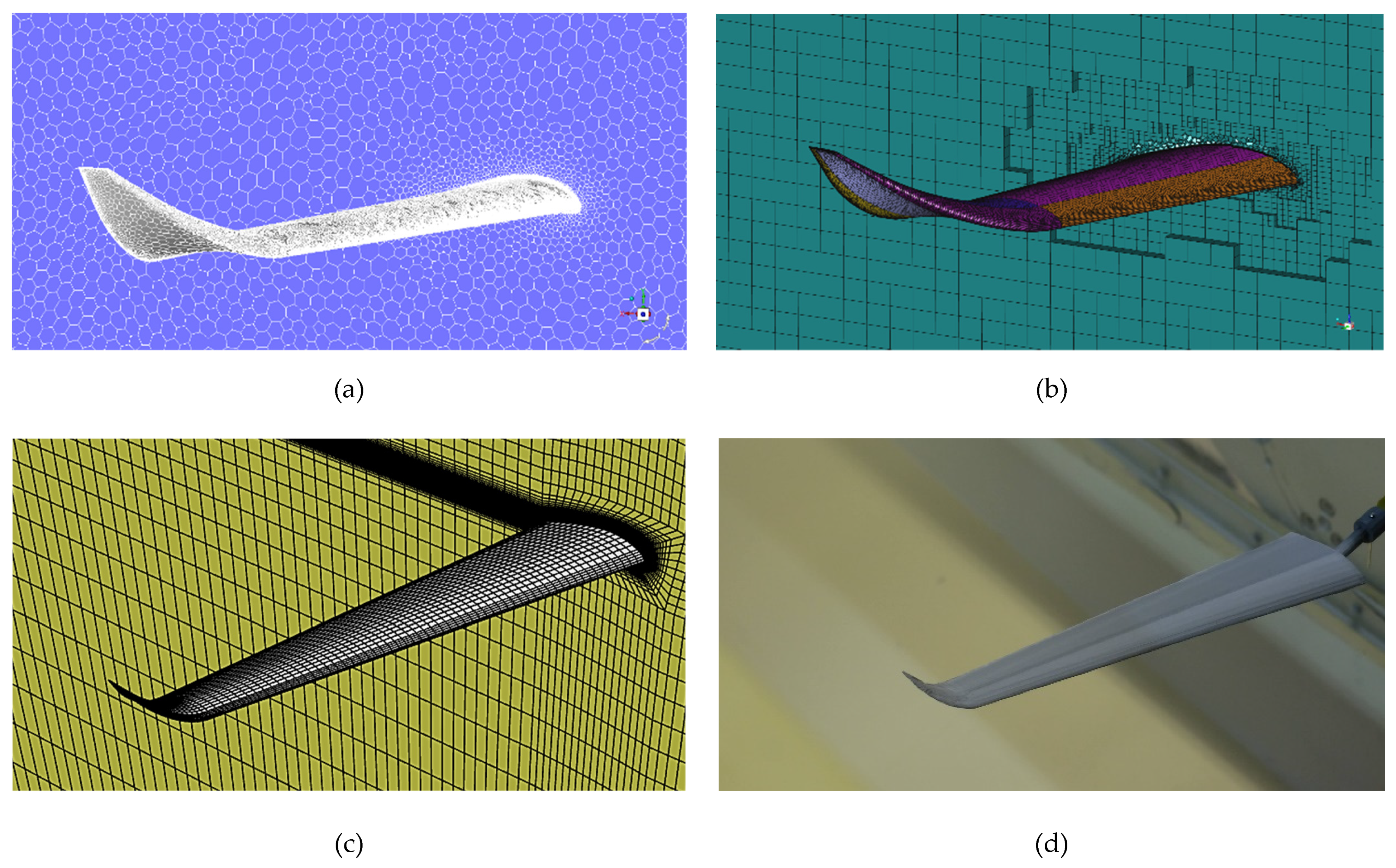
To maximize the accuracy of the results, the computational mesh should be as dense as possible. However, areas far from the geometry have less influence on the results, compared to areas closer to it. Using a denser mesh closer to the wing, accurate results can be obtained, without requiring a prohibitive number of cells. One of the ways this can be achieved is by applying Bodies of Influence (BOIs), i.e., volumes where the grid will be denser. In this study, two BOIs were used, one around the entire wing and one around the winglet. The three final meshes, as exported from the mesh independence study, are presented in Figure 5 followed by the real wing model mounted in the wind tunnel.

Having generated the meshes, the study proceeds with the preparation for the numerical simulation; defining the turbulence model, boundary conditions and the numerical schemes to be utilized. As mentioned earlier in this study, the selected model for all cases of numerical simulations is the SST k-ω. Due to its ability to provide a better prediction of flow separation compared to most RANS models, as well as improved behaviour in adverse pressure gradients, the model selected was considered as preferrable for the simulation of the under investigation wing. Given that the Eppler 420 airfoil is characterized by relatively high camber, in conjunction with the fact that it will be studied in angles of attack of up to 20 degrees, the implementation of this turbulence model was suitable.

For the simulations of the one-phase flow, the solver utilized in Fluent code was the Pressure-based Solver, considering a time-steady airflow, since the flow field conditions can be considered time-independent. Regarding Pressure–Velocity coupling, the Pressure-based coupled algorithm was used to enable a full Pressure–Velocity coupling. The second-order upwind scheme decreases the numerical discretization error; therefore, it was applied to the spatial discretization from the start of calculations. This was mandated by the need for higher accuracy in results for the final comparison to the experimental results, and because of the mesh cell geometries.

Regarding boundary conditions, convergence criteria were set to a class of 1E-6. As a reference temperature 𝑇 =288 K was considered, air density was set to 𝜌 = 1.225 kg/m³, dynamic viscosity was set to 𝜇 = 1.7894 × 10⁻⁵ kg/(ms), with inlet velocity magnitude set to 7 m/s.

For the simulation of the discrete second phase of solid particles, DPM was applied with the boundary condition of reflection on the wing for the solid particles, to more realistically simulate the way particles rebound after impact on the wing. The four walls of the domain were characterized as symmetry at the boundary conditions, and the particles are set to escape in case they reach them after colliding upon the wing.

The discrete phase is considered unsteady and set to interact with the continuous phase and be subject to gravitational forces. Two-way turbulence coupling has been implemented since not only the particles’ behaviour under the influence of the continuous phase needs to be examined, but to also the interaction between them and the changes in turbulent quantities due to particle damping and turbulence eddies. The dispersed entities are modeled as mass-points characterized by a parameter representing their size. Because of the sphericity assumption made for the dispersed entities throughout the present work, they are modeled as a sphere with a diameter, ${\mathrm{d}}_p$, while their volume is given by

$$V_p=\frac{\pi {\mathrm{d}}_p{}^3}{6}$$

(6)

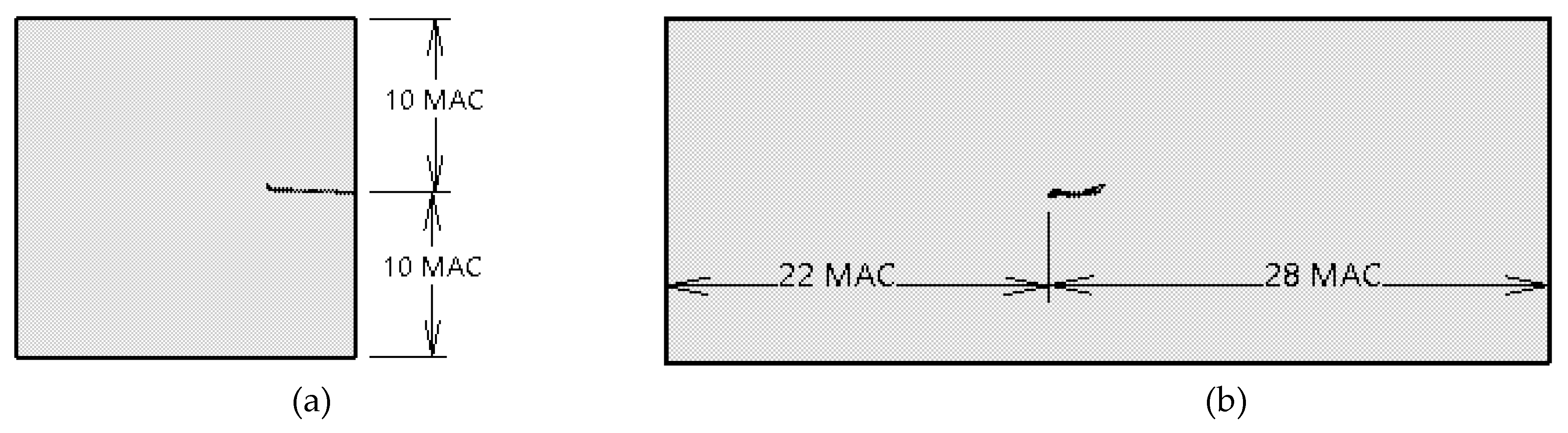
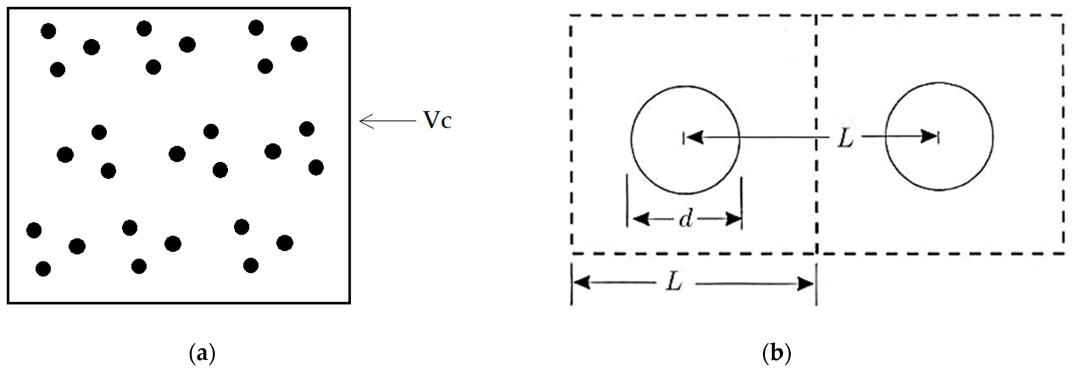
Two quantities that classify the flow pattern are the dispersed phase volume fraction $a_d$ and the entity spacing $L/{\mathrm{d}}_p$. The volume fraction of a number, n, of spherical dispersed entities, with a diameter, ${\mathrm{d}}_p$, in a control volume, $V_C$, is important for the characterization of the two-phase flow from dilute to dense and is defined by

$$a_d=n\frac{V_p}{V_C}=n\frac{\pi {\mathrm{d}}_p{}^3/6}{V_C}$$

(7)

as illustrated in Figure 6a. The characteristic entity spacing $L/d$, illustrated in Figure 6b, of a dispersed second phase in a two-phase flow is defined as the distance $L$ between the middle-points of two adjacent dispersed entities divided by the entity diameter $d$ and can be stated by

$$\frac{L}{d}=\sqrt[3]{\left(\frac{\pi }{6a_d}\right)}$$

(8)

The diameter of the sand particles used for the experiment had a diameter between $0.20 \mathrm{mm}$ and $0.25 \mathrm{mm}$. Thus, a mean diameter $d_{exp}=0.225 \mathrm{mm}$ was assumed for the calculations. Because the volume fraction of the experiment and the numerical simulation should be the same, from Equations (6)–(8) it is obtained:

$$\frac{\pi {\mathrm{d}}_{p,exp}^3/6}{L_{exp}^3}=\frac{\pi {\mathrm{d}}_{p,cfd}^3/6}{L_{cfd}^3}$$

(9)

Since the experiment is a 1:4 scale model of the numerical simulation, all dimensions of the computational domain have been divided by 4. Thus

$$L_{exp}=\frac{L_{cfd}}{4}$$

(10)

As a result, the mean diameter of solid particles, ${\mathrm{d}}_{p,cfd}$, that will be used for DPM is counted to be

$${\mathrm{d}}_{p,cfd}=4 {\mathrm{d}}_{p,exp}=0.9 \mathrm{mm}$$

(11)

For the CFD simulation, the minimum distance between the particles and thus the injections can be found using the volume fraction and must be less than 10% for a dilute flow. From Equation (7), it is obtained that the minimum distance between centres for two neighbouring solid particles is

$$L_{cfd,min}=0.00156 \mathrm{m}$$

(12)

Through trial and error, it is found that an injection surface with the shape of a rectangular parallelogram, measuring 𝑌 × 𝑍 = 760 mm × 180 mm, was adequate for full coverage of the wing by the second phase. Moreover, it was decided to use a distance of $L=0.02 \mathrm{m}$ between injections, higher than the minimum allowable (12), to keep simulations time reasonable, even though a smaller value would yield more accurate results. Using this distance, it is calculated that 39 injections will have to be applied in the Y-direction and 10 in the Z-direction, deriving a total of 390 injection points.

Therefore, the second phase injection into the airflow was inserted by a spray surface perpendicular to the airflow, from 390 injection points in a timestep of 0.005 s. As previously referred in this work, the numerical simulations were first conducted using sand particles as the discrete phase. The medium dry sand, used for both the first numerical simulations and the experiment, has a mean density of 1500 kg/m³. Afterwards, the same simulations were executed using anthracite particles as the dispersed phase, with a density of 1550 kg/m³.

Every 0.005 s, a parcel consisting of 390 particles is injected. This translates to an injection of 200 parcels per second, or 78,000 particles per second, both for the sand and anthracite cases. The average mass flow of solid phase imported to the airflow is equal to 44.66 g/s and 46.15 g/s, for sand and anthracite cases, respectively. Particle velocity in the horizontal direction for an angle of attack of 0° was set equal to air velocity, i.e., u = 7 m/s, while particle velocity in the vertical direction for angle of attack 0° was chosen to be w = 1 m/s, in an effort to simulate the upward motion of combustion particles during a wildfire. The composition of smoke from a forest fire appears to be quite complex, containing numerous components such as carbon dioxide, carbon monoxide, methane, and others. Such modelling would be beyond the scope of this research; thus, it was decided to use anthracite as the solid particle material, due to its high carbon concentration.

3. Experimental Procedure

For the experimental study, the wind tunnel of the Fluid Mechanics and Fluid Applications Laboratory, Patras University, was used, inside which the experimental model of the wing was placed, at a scale of 1:4 [17]. The wind tunnel is a BLOWER TUNEL model constructed by Plint & Partners Ltd. Engineers in 1977. It is an open-type wind tunnel, i.e., the flow is discharged into the air immediately after the measurement chamber. This results in operation at a pressure approaching atmospheric pressure, in addition to facilitating access to the model. The measuring chamber has dimensions of 1.7 × 0.65 × 0.65 m and is equipped with three Plexiglas windows with removable frames, allowing easy access to the model, as well as visual contact. To derive the coefficients of lift and drag of the experimental model, the three-component AFA3 aerodynamic balance from TQ Education and Training Ltd. was used, as shown in Figure 7, a device that measures two forces (lift and drag) and a moment (pitching moment). The display module mounts onto the wind tunnel control and instrumentation frame, and includes a digital display to show the lift, drag and pitching moment directly. To affix the model to the aerodynamic balance, a shaft of 12 mm diameter and 220 mm length is used, placed in the socket of the balance retaining mechanism and secured by a special tightening bolt. In addition, the restraint mechanism is calibrated on the circumference and is free to rotate through 360°. Thus, the possibility to precisely adjust the model’s angle of attack is given and immobilize it in the desired position, with the help of the appropriate screw.

The aerodynamic balance is compatible with an appropriate software, TecQuipment’s Versatile Data Acquisition System (VDAS), and can quickly and conveniently connect to a frame-mounting interface unit. Using VDAS enables accurate real-time data capture, monitoring, display, calculation and charting of all relevant parameters on the Laboratory’s computer. This equipment may be characterized of adequate precision, since it can count forces with second decimal precision, while its capacity is 100 N for lift, 50 N for drag and 2.5 Nm for pitching moment. For every angle of attack examined, a set of force measurements was collected. Through the software, a time step to record the values was set to 0.2 s. It was chosen to keep each angle of attack constant for at least 300 s during the operation of the wind tunnel, in order to reduce the margin of error during the recording of the values. After each period of 5 min, more than 1500 values were recorded. These were collected for each angle of attack and were first checked for possible outliers that might affect the mean value, before calculating the mean values of forces for every case.

As mentioned above, the two-phase flow of combustion particles and their upward movement would be experimentally simulated by medium sand grains spread on an inclined base, due to safety limitations. In this way, the wind would carry the sand grains at the correct angle to hit the scaled wing. The experimental setup is shown in the schematic diagram of Figure 8a, and the operational wind tunnel air flow velocity is set at 27 m/s, four times higher than the respective value for the numerical simulation, aiming to obtain the same Re number as the numerical simulation.

In Figure 8b, the region of spray surface chosen and the motion of solid particles, under the influence of air velocity, may be seen. It is also observed that after approximately 0.5 s, the first solid particles have reached the wing and have interacted with it.

4. Results

The main scope of meshing was to develop a domain with a large number of nodes, with densification of the grid mesh around the wing section. The first section of the study included the comparison of results arising from the numerical simulation under the three different meshing techniques—those of a completely structured mesh, an unstructured mesh and a poly-hexcore mosaic mesh—both for the case of one-phase flow, as well as the two cases of two-phase phase flows; with sand particles and anthracite particles as discrete phase Moreover, the results from the one phase flow, and the two-phase flow with sand, were intended to be compared with the results gained from the experiment conducted at the subsonic wind tunnel.

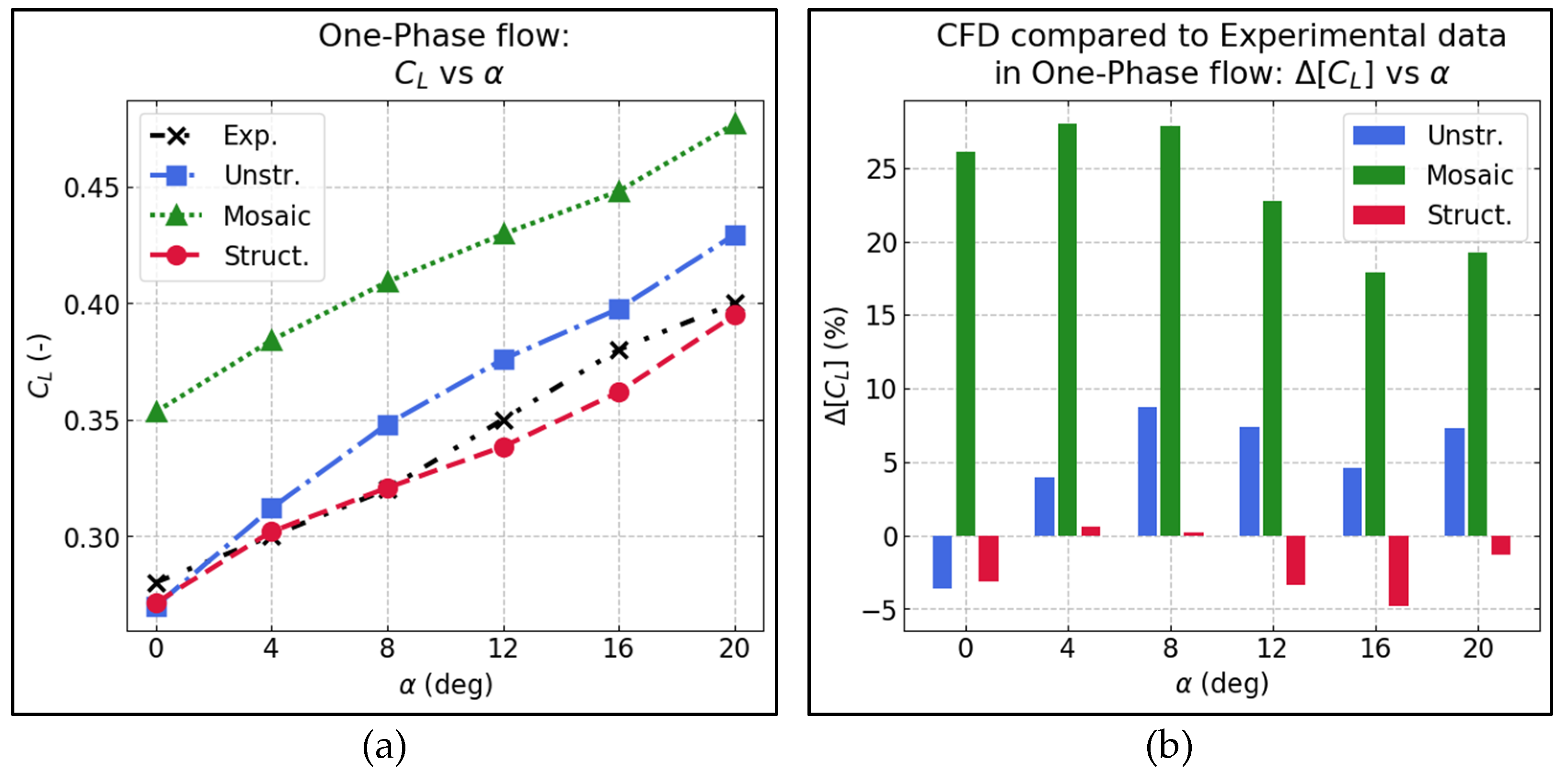
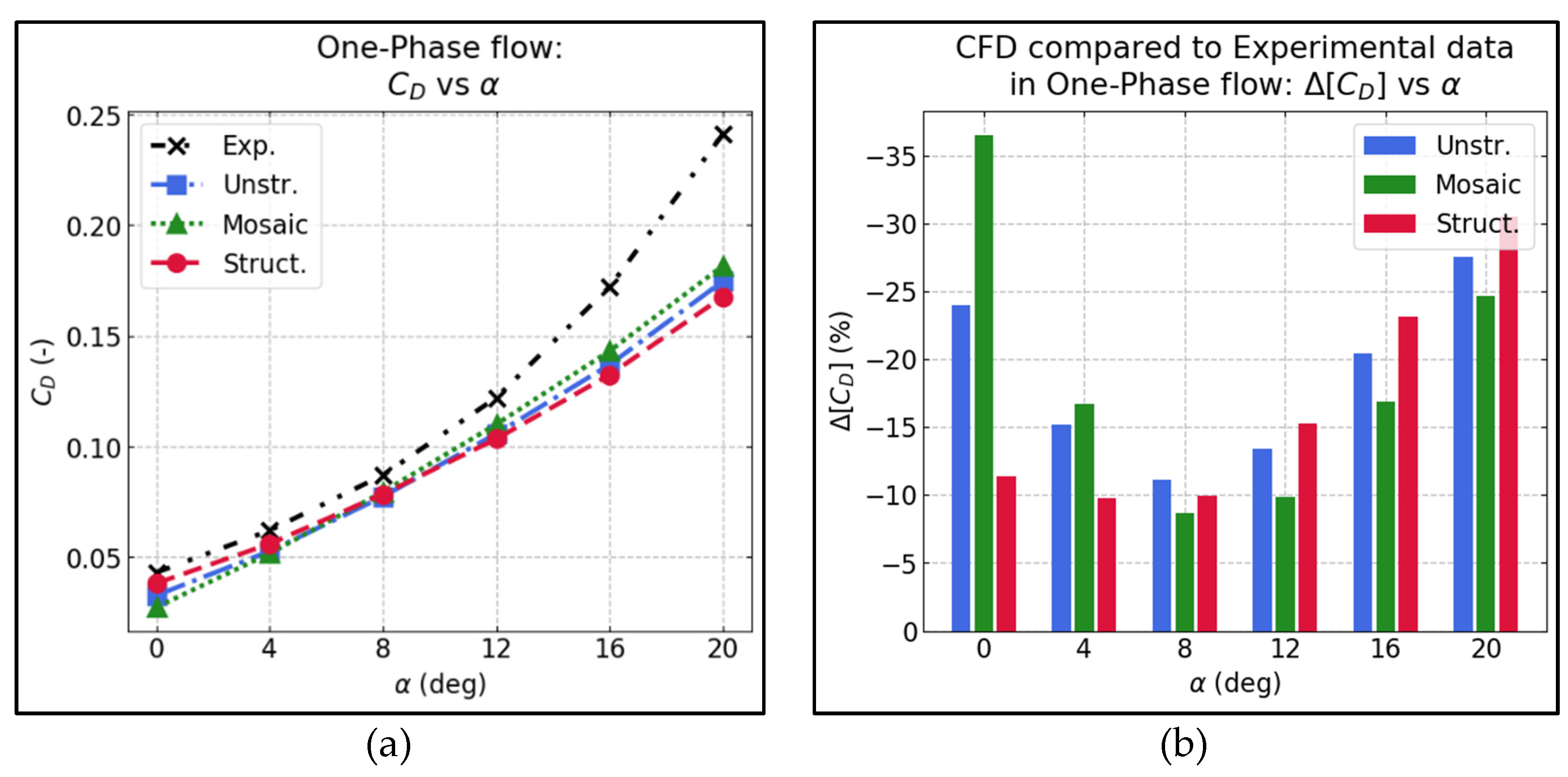
As observed in the following charts of Figure 9, the results of the mosaic poly-hexcore mesh simulation are, in general, more aerodynamically optimistic than both the other two cases, and the experimental results. A deviation of approximately 26% higher lift coefficient is observed as compared to the other numerical simulations, while the drag coefficient, see Figure 10, is again higher than in the other cases of numerical simulation, but at a radically lower level. On the contrary, the structured mesh simulation showed both a lower lift coefficient and a lower drag coefficient than the other two cases of simulation, more precisely approaching the experimental results, as expected.

On average, following comparison of each different meshing technique simulation with results obtained from the wind tunnel experiment, it is discerned that the lift coefficient of the mosaic poly-hexcore showed a mean deviation of approximately 24%, while the unstructured and structured showed 6% and 2.5%, respectively.

Concurrently, the results regarding drag coefficient show a similar behaviour. The numerical simulations for all three mesh techniques showed a more optimistic aerodynamic behaviour compared to the results exported from the wind tunnel. Specifically, the experimental results showed a higher drag coefficient compared to all three simulations, and deviation increased for higher angles of attack between 12 and 20 degrees. Again, the lowest mean deviation compared to experimental results was shown from the structured mesh simulation, at approximately 16%, while mosaic and unstructured both had a divergence of about 19%.

The above lead us to an early conclusion, that the mosaic poly-hexcore mesh gives relatively higher values for lift coefficient when compared with the other two meshes and the experimental results, while regarding drag coefficient, the three different meshes have a strong convergence between each other but show a relatively notable divergence from the experimental results.

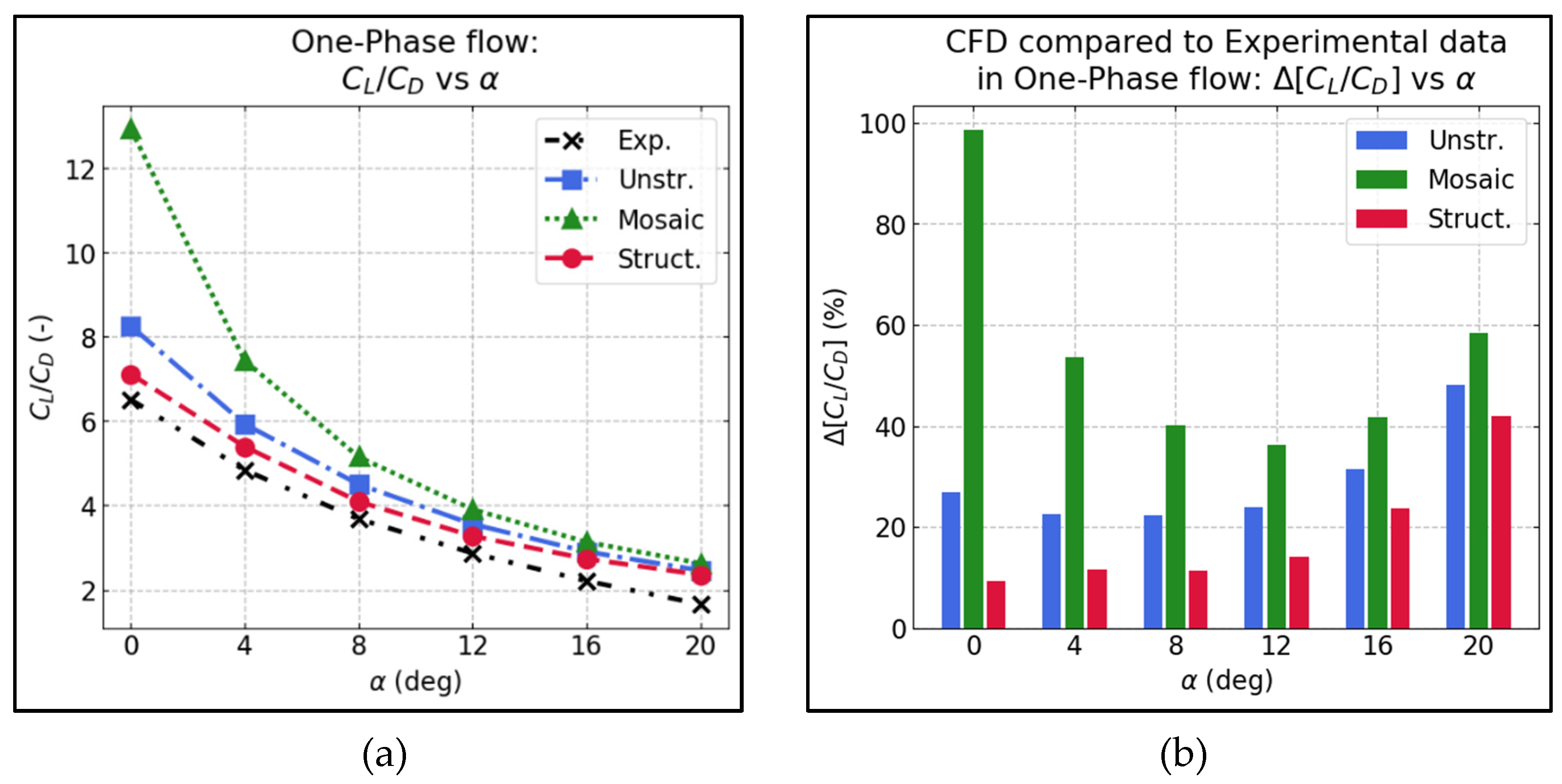
All the above-mentioned results and conclusions for the one-phase flow are summarized in the charts of Figure 11, where the aerodynamic efficiency for each case is illustrated. For every simulation with an angle of attack ranging between 0 degrees and 20 degrees, the mosaic mesh showed the most optimistic aerodynamic performance.

Furthermore, despite the fact that the three mesh techniques’ simulations showed a divergence for 0 degrees, they concluded to a significant convergence at 20 degrees. Last but not least, the aerodynamic efficiency exported from the experiment was, for all angles of attack, lower than those of the three simulations. As expected, the simulation that approached the experimental results with greater precision was that of the fully structured mesh, while the mosaic mesh simulation was that with the highest divergence compared to the experimental results.

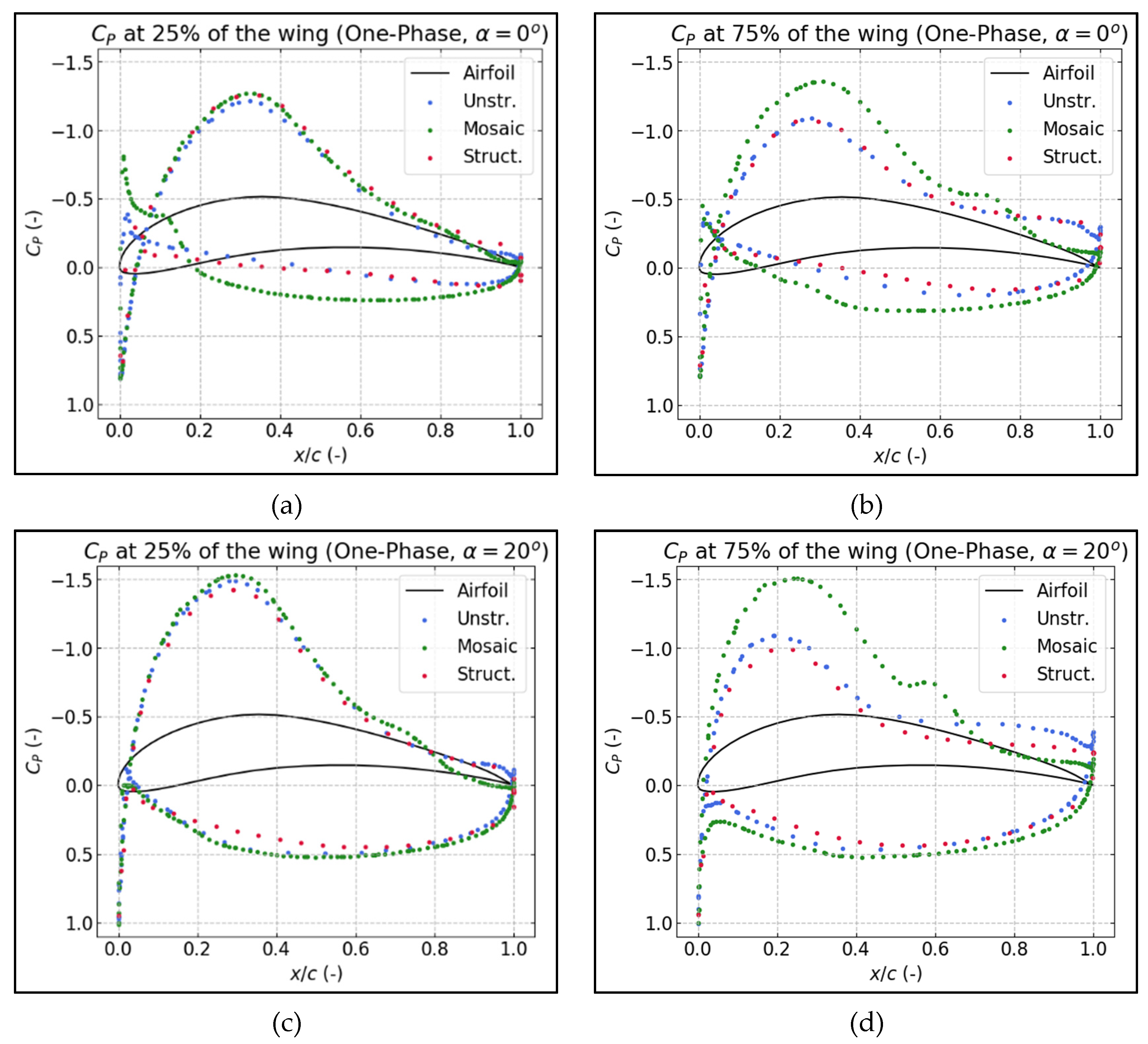
Simultaneously, the research proceeded with the extraction of pressure coefficient (C_p) distribution over airfoils of the wing, for all the three meshing techniques. The airfoils selected were located at 25% and 75% of the wingspan, in order to examine the differences along its length. Moreover, these airfoils were investigated in two different angles of attack, 0 and 20 degrees. As observed in Figure 12, regarding the airfoil at 25% of the wingspan, the pressure coefficient from the mosaic mesh is higher for the lower surface, whereas for the upper surface there is a very good agreement for the coefficient exported from all three different meshes. This fact explains the higher lift coefficient from the mosaic poly-hexcore mesh.

However, this does not happen for the airfoil at 75% of the wingspan. At this location, for both angles of attack, 0 and 20 degrees, the C_p from mosaic mesh shows significant divergence from structured and unstructured mesh C_p. All these results justify the more optimistic aerodynamic performance of the mosaic mesh study, presented in the previous section of this work. As already expected, the larger the angle of attack, the greater the difference of pressure coefficient between the lower and upper surface. The difference of pressure coefficient is significantly higher on the front edge compared to the rear edge, indicating that the airfoil’s lift force is mainly generated from the front edge.

Significant results about the flow separation and reattachment may be exported by the C_p distributions, explaining the differences among the three meshing configurations. More thoroughly examining the plots of C_p distribution at 75% of the wingspan and 0 degrees angle of attack, the structured and unstructured meshes appear to predict a flow separation at x/c~0.5, while the mosaic mesh exhibits a separation point at x/c~0.6. Notably, the flow at the mosaic mesh appears to reattach at the upper surface of the airfoil at x/c~0.8. A similar behaviour is demonstrated in the plot of Figure 12d, where the structured mesh shows a separation point starting at x/c~0.4, slightly earlier than that observed for the unstructured mesh. Again, the mosaic mesh exhibits a later flow separation, at x/c~0.5, and, judging by the plot, a temporary reattachment occurs at x/c~0.7, until the final boundary layer separation. A common point for all meshing configurations is that with the increase in angle of attack, the flow separation moves towards the leading edge of the airfoils, both at 25% and 75% of the wingspan.

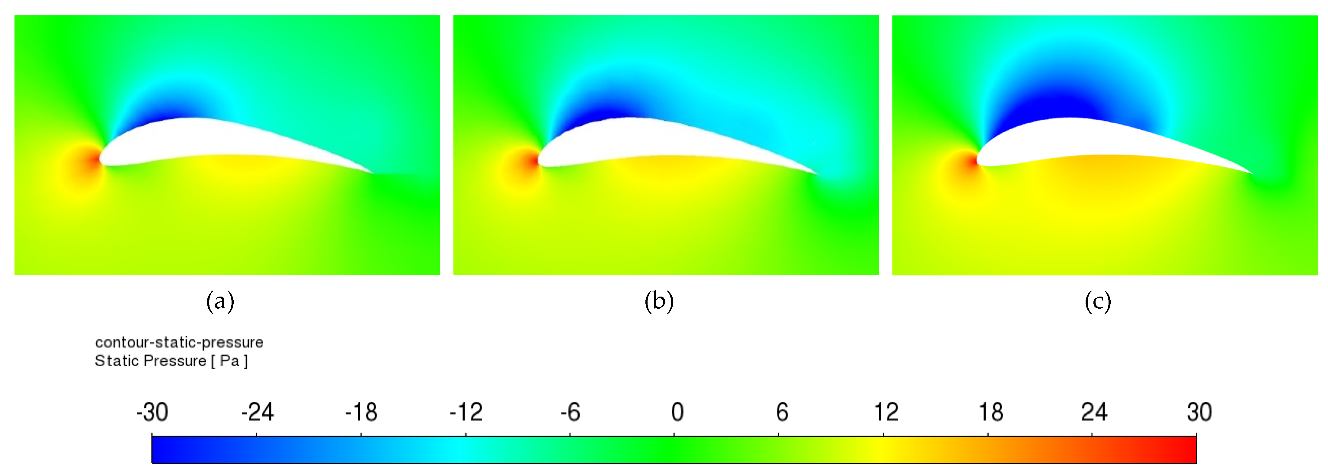
This aerodynamic behaviour is even better represented by Figure 13, portraying static pressure distribution at 75% of the wingspan for the three meshing techniques. It is easily understood by the colour scale that the difference of static pressure between lower and upper surfaces is higher for the mosaic mesh study than the other two.

An overview of the results, presented in C_p distribution plots, is also included here. Structured and unstructured meshes appear to predict a separation point at nearly 40% of the chord, while the mosaic mesh predicts it at 50% of the chord. It must be noted that reattachment seems to appear until final separation, in the region between 50% and 70% of the chord, as shown in Figure 13c.

As expected, the pressure gradient from the mosaic mesh is higher, which results in higher lift values compared to the other two meshes, followed by the unstructured mesh with slight differentiation by the structured mesh.

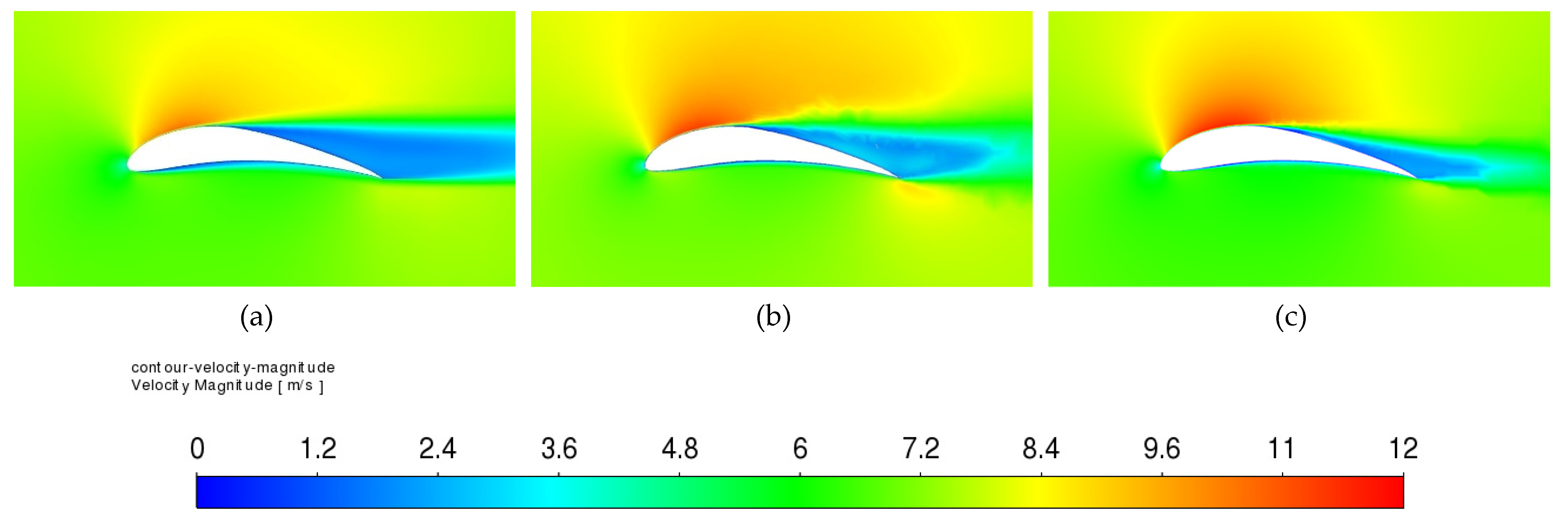
The same pattern is exhibited by the contours of velocity distribution for the same location and angle of attack. In Figure 14, the decelerating flow for the structured and unstructured meshes is observed at a spot close to 40% of the chord, followed by flow separation which continues until the trailing edge. The unstructured mesh seems to produce a thicker boundary layer compared to the structured mesh, as well as higher velocity values that justify the higher pressure gradient and lift values obtained. However, both form a thinner boundary layer compared to the mosaic mesh, where the flow appears to decelerate at a point close to 50% of the chord. If Figure 14c is closely observed, and particularly the section between 50% and approximately 70% of the suction surface, a separation bubble appears spanning nearly 20% of the airfoil. After this, there is a temporary reattachment of flow, described above, and then flow separation which continues until the trailing edge.

The study continued with the research on the two-phase flow, consisting of two stages of comparison/validation. In the first part, numerical simulations of two-phase flow with solid particles of sand were executed. These results were compared with the experimental results of the two-phase flow of air–sand, conducted in the wind-tunnel. After obtaining good agreement between computational and experimental results, the study continues with the second part, which includes the execution of numerical simulations of two-phase flow with anthracite particles.

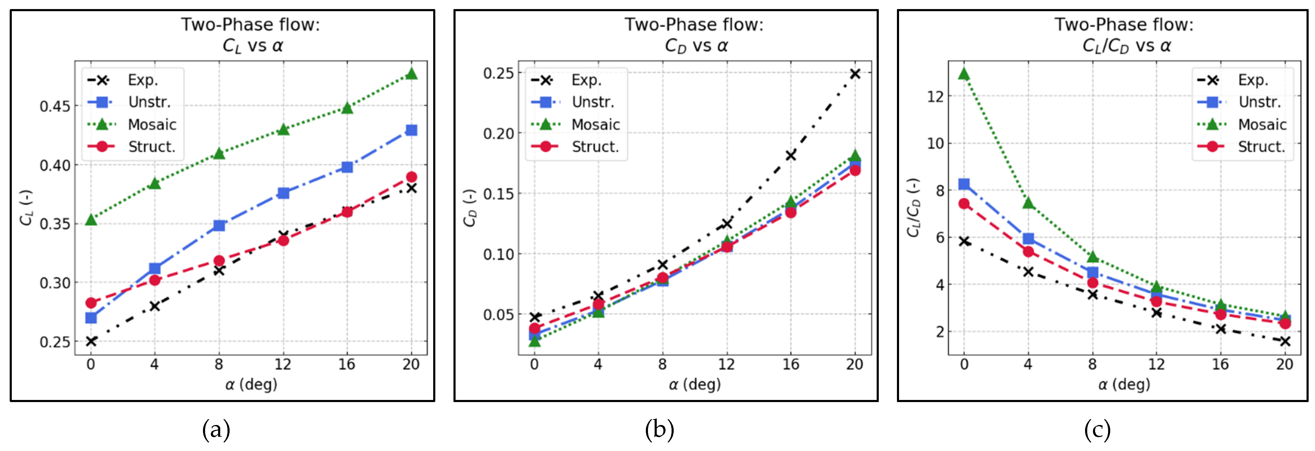
The two-phase flow was simulated by a continuous phase of airflow, while the second phase was simulated by the injection of solid particles. The results, presented in Figure 15, again showed a significant divergence of the results of the mosaic poly-hexcore mesh compared to the other two mesh techniques, regarding both the lift and drag coefficients, as well as a generally more optimistic aerodynamic behaviour compared to experimental results. The structured mesh simulation gave the most precise results compared to the experimental results for both coefficients. When compared to experimental results, the lift coefficient of the mosaic poly-hexcore mesh simulation had a mean deviation of 30%, while the structured mesh simulation had a mean deviation of 4%. Similarly, the drag coefficient calculated from the experiment was, in general, higher for all angles of attack compared to the CFD simulations with all three mesh techniques. Again, the structured mesh simulation had the lowest divergence for the drag coefficient, at approximately 19%, while the mosaic poly-hexcore and the unstructured mesh simulations showed a mean divergence of approximately 22% each, compared to the drag coefficient calculated experimentally.

The same phenomenon that appeared in single phase flow also appeared in the two-phase flow, that of tendency for higher divergence of experimental drag coefficient compared to the numerical simulations’, for angles of attack of 12 degrees and higher. It must be underlined that, similarly to the single-phase flow, the C_L/C_D ratio of the experimental results was lower compared to all three numerical simulations, for all degrees of angle of attack in the two-phase flow. Moreover, it is observed that the divergence of aerodynamic efficiency for the numerical simulations at 0 degrees results in very good convergence for an angle of attack of 20 degrees.

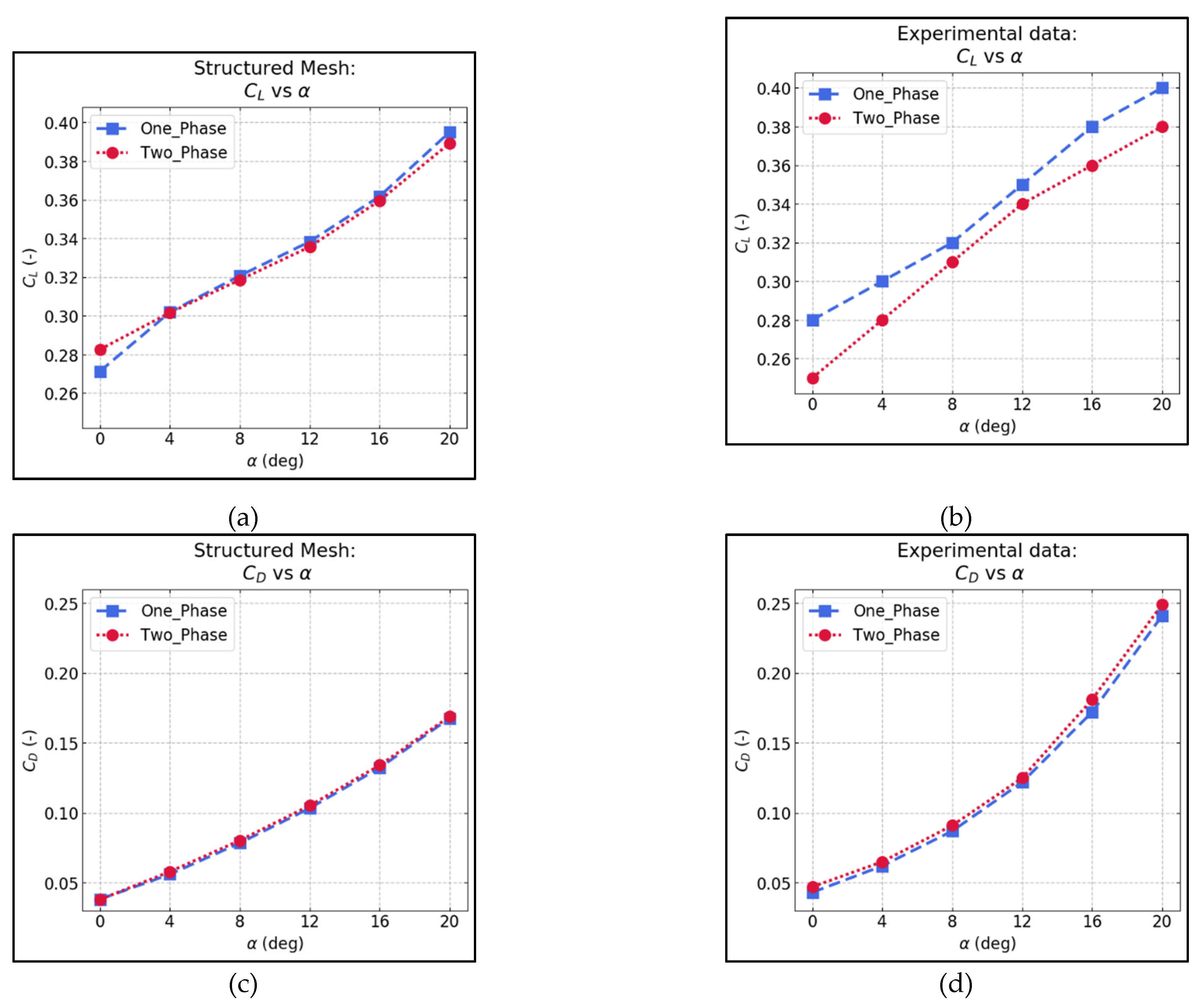
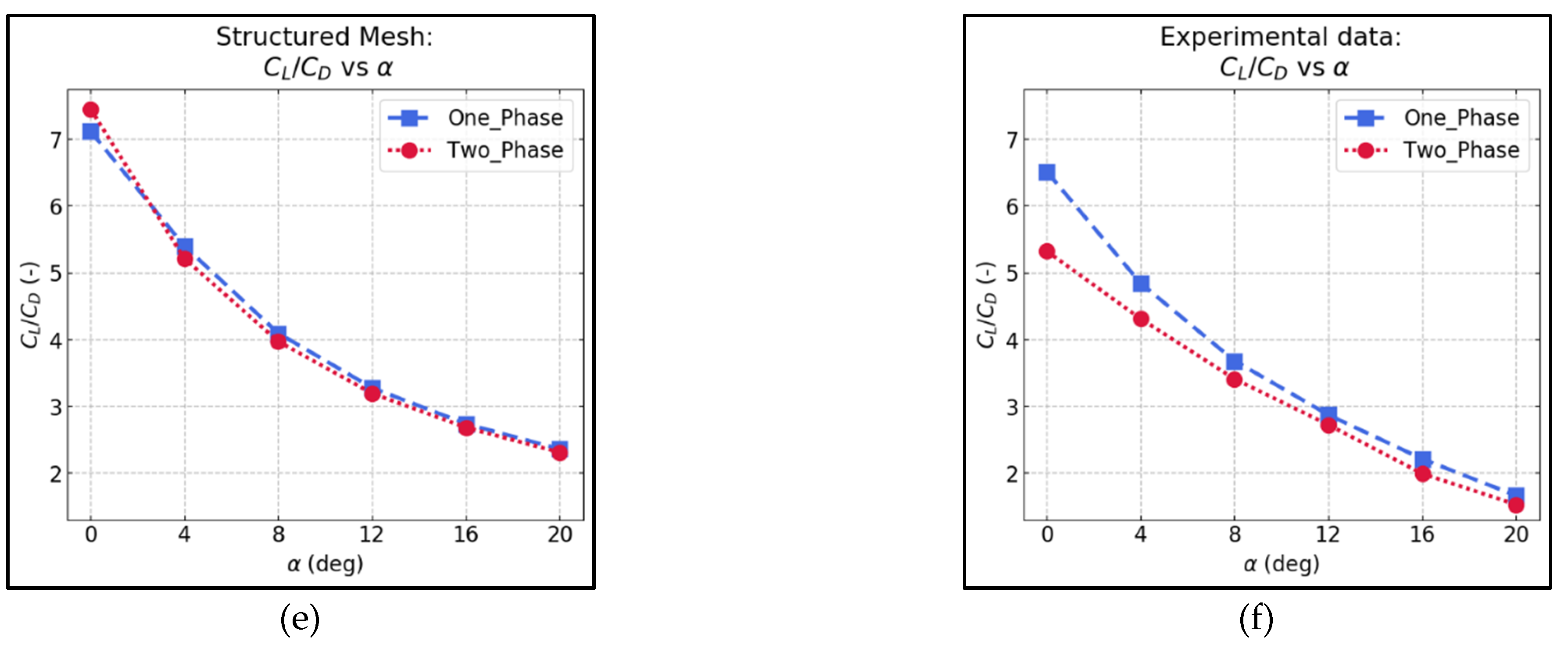
After the end of the demonstration of the first section of results, this study proceeded with the investigation of whether and in which amount the aerodynamic behaviour of the wing is influenced by the existence of the solid particles in the airflow stream. Since the structured mesh technique simulation led to more accurate results closer to the experiment, in this section, the demonstrated results will be with this meshing technique. As expressed in the literature, it is generally expected that the presence of a second flow of different phase substance influences the aerodynamic behaviour of the wing in a negative way. The following charts in Figure 16 illustrate the results from the numerical simulation with the structured mesh. A slight degradation of the aerodynamic efficiency is observed. Specifically, the one-phase flow lift coefficient shows a higher value at the angle of attack of 0 degrees and for the rest simulations is lower compared to two-phase flow lift coefficient. That is represented in Figure 16a and the average decline calculated is 1.3%. Similarly, the single phase drag coefficient, in Figure 16c, shows a lower value at 0 degrees and for the rest simulations is slightly higher. The mean increase, due to the existence of the second phase, is calculated 1.8%. As a result, the aerodynamic efficiency, in Figure 16e, follows the same pattern. Except for the case of a 0-degree angle of attack, where there is an increase of 2.9%, for all the rest of the angles of attack, a general decline, approximately 3%, is observed. An interesting fact that should be mentioned is that the highest divergence is observed at an angle of attack of 4 degrees and after this case, the divergence of the aerodynamic efficiency is lowering with the increase in angle of attack.

A similar performance is observed during the experiments at the subsonic wind tunnel. The common prediction of degradation, due to the second phase, is again verified but to a larger extent compared to numerical simulations’ results. More specifically, the two-phase flow lift coefficient is lower than the corresponding in single phase flow, during all cases of angles of attack, with an average decrease of approximately 5.6%. At the same time, the drag coefficient of two-phase flow is permanently higher than that of single phase with an average deviation of approximately 4.96%. It is easily understood that these results lead to an average degradation of the aerodynamic efficiency at an amount of 9.98%. This means that the wing, in case it flies inside a two-phase flow with the same characteristics to our experiment, faces a loss of 1/10 of its aerodynamic efficiency.

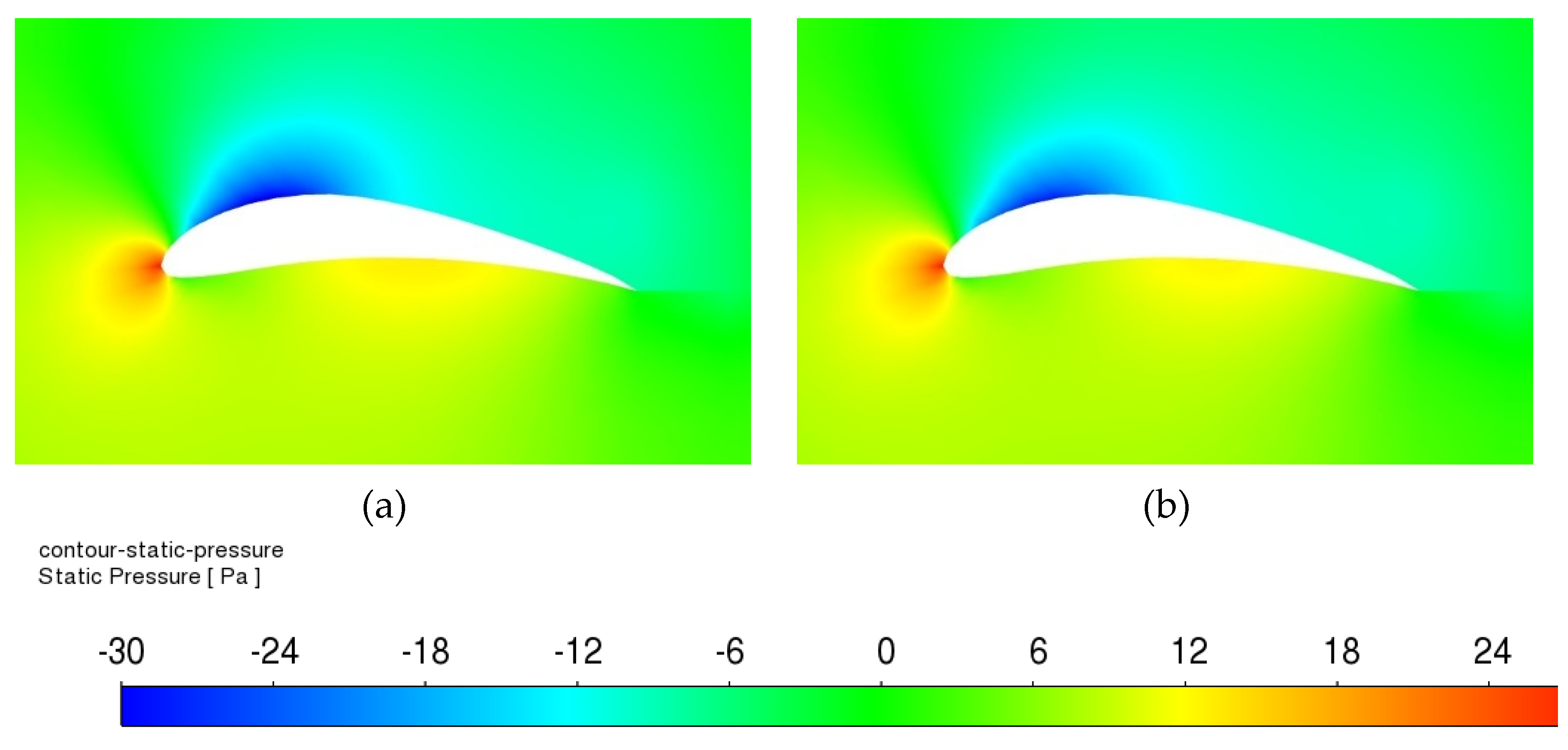
The static pressure distribution is shown in Figure 17, as this was exported from the structured mesh numerical simulations, for both one-phase and two-phase flows. The airfoils chosen are located at the 75% of the wingspan, with angle of attack of 20 degrees. It should be underlined that the pressure difference between upper and lower surface is declined for the two-phase flow when compared to one-phase flow. This leads to the result of the lift and the lift-to-drag ratio decreasing with the existence of the second phase.

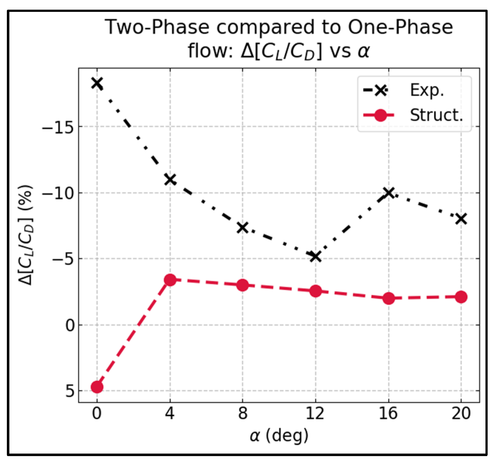
In

Table 3. L/D percentage degradation due to the existence of second phase (sand).

Angle of Attack (°)	Aerodynamic Efficiency Degradation (Experiment)	Aerodynamic Efficiency Degradation (Structured Mesh)
0	−18.3%	4.70%
4	−11.0%	−3.43%
8	−7.4%	−3.00%
12	−5.2%	−2.55%
16	−10.0%	−2.00%
20	−8.1%	−2.11%

and Figure 18, L/D degradation is presented for the numerical simulation for the structured mesh as well as for the experiment conducted in the subsonic wind tunnel. The general tendency shown is the decline of the aerodynamic efficiency due to the presence of the solid phase. There is a slight disagreement between the experiment and numerical simulation for an angle of attack of 0 degrees. During the experiment, the highest percentage degradation, −18.3%, appears at 0 degrees, while this occurs at 4 degrees for the numerical simulation and is calculated −3.43%. After 4 degrees and until 12 degrees, both cases present the same behaviour, that of a decrease in percentage degradation, −11% to −5.2% and −3.43% to −2.55%. After 12 degrees, the results from numerical simulation continue showing a decrease with a tendency to stabilize at a percentage of -2% due to the existence of sand particles in contrast with the experiment. Finally, at 16 degrees, degradation increases to −10% and at 20 degrees is reduced to −8.1%. What needs to be mentioned here is that the two-phase flow simulation concluded to more optimistic aerodynamic results compared to the experimental procedure regarding the percentage degradation of aerodynamic efficiency.

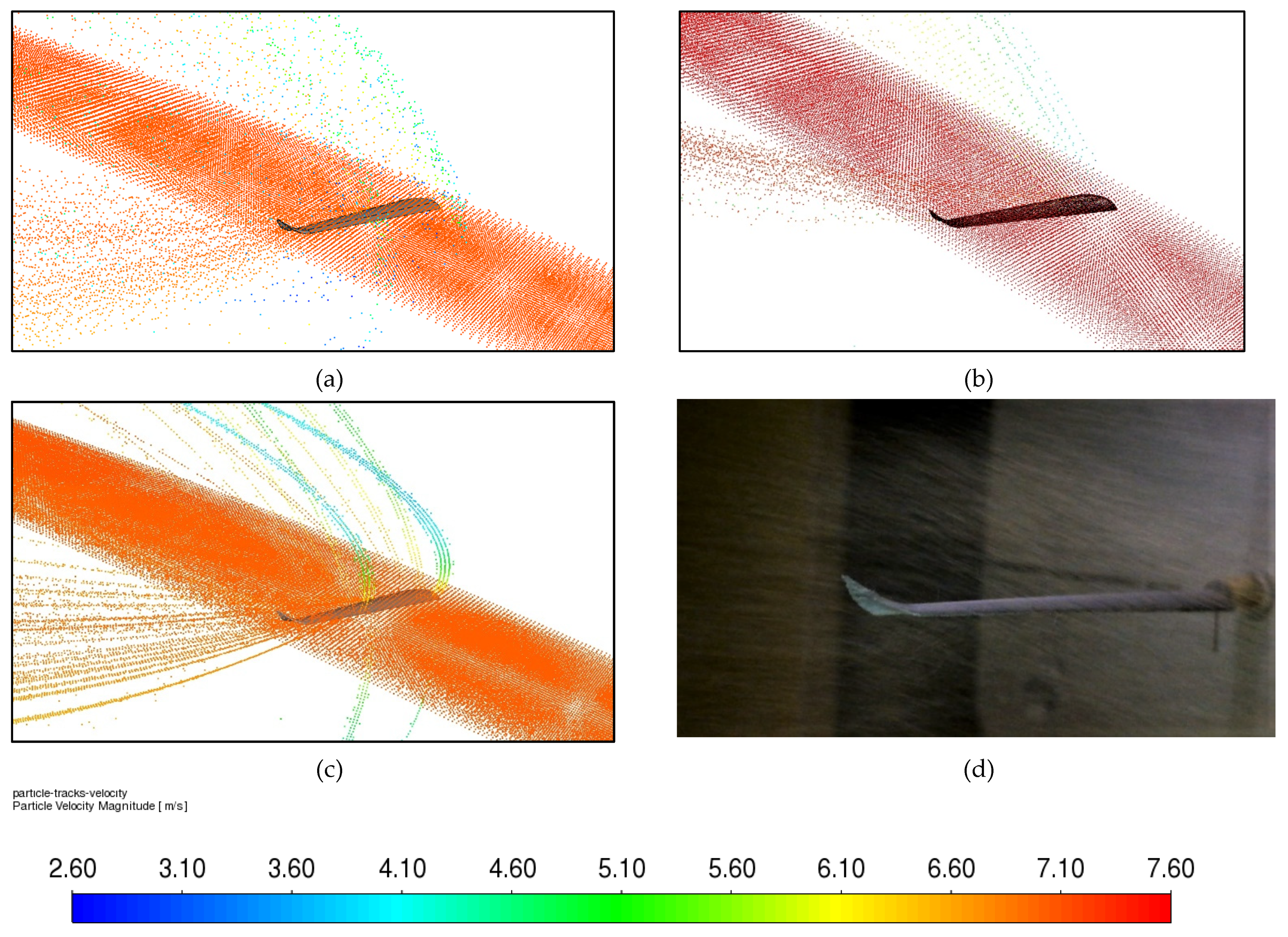
Figure 19 shows the solid particles’ trajectories and velocity magnitudes obtained from the numerical simulation in Ansys Fluent and a snapshot captured during the two-phase flow experiment conducted at the subsonic wind tunnel. There is an amount of sand particles injected in the airflow which collide with the wing and rebound off, having a change in their velocity vector.

However, this phenomenon does not appear in the same way for the three meshing configurations. In the structured mesh simulation, the sand particles that reflect on the wing appear to formulate flow streams when carried away by the free airflow stream, at the region above the wing. This does not happen with the other two meshes, where the particles, after their impact on the wing, move backward in a dilute cloudy behaviour. In all pictures, however, the unregulated flow of solid particles after leaving the wing area may be noticed.

Comparing with the snapshot from the experimental procedure, though, the fact that the behaviour of particles’ movement shows similarities with all three meshes simulations could be concluded, especially regarding the behaviour after the impact on the wing and the irregularities in the flow after it.

After the validation of the two-phase flow numerical results with the experimental results, both conducted with the use of sand as solid phase, the study proceeds with the last part of the research. In this part, the numerical simulations of two-phase flow were again conducted, but this time with the implementation of anthracite as second phase. The final scope is to compare these results with the validated results. Via this two-stage comparison, safe conclusions, to what extent the results that came from the numerical simulations with anthracite are reliable, may be drawn.

The results from all two-phase numerical simulations are gathered in

Table 4. Lift and drag coefficients of two-phase flow with sand and anthracite and their percentage deviation, for the three meshes.

Grid	Angle of Attack (Degrees)	CL (-) (DPM Sand)	CL (-) (DPM Anthracite)	CL Deviation (%) (Sand vs. Anthracite)	CD (-) (DPM Sand)	CD (-) (DPM Anthracite)	CD Deviation (%) (Sand vs. Anthracite)
Unstructured	0	0.26971	0.28580	5.97%	0.03271	0.03187	−2.57%
	4	0.31165	0.32125	3.08%	0.05260	0.05248	−0.23%
	8	0.34798	0.35258	1.32%	0.07733	0.07731	−0.02%
	12	0.37578	0.37849	0.72%	0.10569	0.10567	−0.02%
	16	0.39759	0.39978	0.55%	0.13689	0.13677	−0.08%
	20	0.42940	0.43055	0.27%	0.17461	0.17456	−0.03%
Mosaic Poly-Hexcore	0	0.35331	0.35334	0.01%	0.02732	0.02732	−0.01%
	4	0.38407	0.38406	0.00%	0.05163	0.05165	0.03%
	8	0.40914	0.40918	0.01%	0.07943	0.07944	0.01%
	12	0.42962	0.42964	0.00%	0.10996	0.10997	0.01%
	16	0.44814	0.44819	0.01%	0.14305	0.14304	−0.01%
	20	0.47698	0.47701	0.01%	0.18153	0.18151	−0.01%
Structured	0	0.28255	0.28260	0.02%	0.03793	0.03752	−1.07%
	4	0.30159	0.30175	0.05%	0.05788	0.05793	0.09%
	8	0.31855	0.31859	0.01%	0.08027	0.08029	0.02%
	12	0.33563	0.33561	−0.01%	0.10521	0.10520	−0.01%
	16	0.35956	0.35960	0.01%	0.13416	0.13411	−0.04%
	20	0.38917	0.38990	0.19%	0.16871	0.16910	0.23%

. The results are divided in three sections, one for each different meshing configuration. Analyzing, firstly, the results for the lift coefficient, it is obvious that especially for structured and mosaic mesh, the deviations are almost zero. For structured mesh the maximum deviation occurs at 20 degrees and is calculated 0.19%. The convergence is even greater for the mosaic mesh, where there is practically no divergence, as it is as low as 0.01%. Slightly higher divergences are found in the unstructured mesh results, where they range from 0.27% to 5.97%. However, considering that in the two-phase simulation with sand, it was the structured mesh that gave the closest values to the experimental ones and that simulation with anthracite shows deviations of less than 0.2%, it can be claimed that the initial hypothesis is verified to an excellent level.

The same pattern is exhibited if the drag coefficients from simulations with sand and anthracite are compared. Unstructured mesh shows deviations from −2.57% to −0.02%. Mosaic mesh again shows practically no divergence. Structured mesh simulation results appear to have deviation in a range between −1.07% and 0.23%, when comparing the two-phase flow with sand and anthracite. Based on this result, it can, once again, be claimed that the initial hypothesis has been verified.

5. Discussion and Conclusions

In this study, the preliminary design from scratch of a wing with specific aerodynamic characteristics was carried out, for use in a firefighting UAV. The wing was based on the Eppler 420 airfoil and was designed to have a sweep angle, a dihedral angle, taper along the span and a custom-designed blended winglet attached to the wingtip. The aim of the research was, in the first stage, to study its aerodynamic behaviour in the commercial Ansys Fluent simulation code at speed under Re = 65,000 and at various angles of attack, in both one-phase airflow and two-phase air–embers flow. Subsequently the aim was to perform an experiment, in a subsonic wind tunnel, at boundary conditions identical to those of the numerical simulations, both in one-phase and two-phase flows. Due to Laboratory safety limitations, the embers from the two-phase experimental procedure were simulated with medium sand. The two-phase numerical simulation was first conducted with sand as the second phase, and the results were compared with the experimental results. For the final validation, the two-phase simulation was again conducted with anthracite as the dispersed phase, the composition of which more closely approximates the solid products of fire. The results were then compared with the validated results from the two-phase flow with sand.

Concurrently, an attempt was made to create a mesh with three different meshing configurations. The first intention was to compare the results and to draw conclusions as to which, among the three, best approximates the experimental results. The second target was to estimate the behaviour of the same model in these different meshes, and to extract results about differences in aerodynamic behaviour.

Initially, a fully structured mesh, an unstructured mesh, and a relatively new configuration, that of the mosaic poly-hexcore mesh, were generated. The one phase flow simulations showed that the mosaic mesh produced, in general, more optimistic aerodynamic results than the structured and unstructured meshes. This may, partially, be justified by observing the diagrams of pressure coefficient distribution along the wingspan. Moving from the wingroot towards the wingtip, and independently from the angle of attack, C_P produced from the mosaic mesh exhibits notable divergence compared to the other two configurations, obtaining higher values. For the entire range of angles of attack, the structured mesh results of aerodynamic efficiency were closer to the experimental results. With the increase in angle of attack, a significant convergence appeared for the three different mesh configurations. It may be concluded that all three different mesh building architectures showed relative convergence with one another. However, as expected, the structured mesh distinguished itself for having the lowest deviation from the experimental results.

Concerning the first case of the two-phase flow study, the results showed that the presence of sand particles in the flow resulted in a degradation of the aerodynamic performance of the wing at an average rate of almost 3% for numerical simulation, and almost 10% for experimental study. The differences in static pressure distribution around the wing between one-phase and two-phase flows demonstrates this aerodynamic decline. It is worth mentioning that this degradation was intensified at lower angles of attack, while it showed signs of convergence while increasing the angle of attack. In overall, the structured mesh numerical simulation had once more a good agreement with the experimental procedure and was the one to better predict aerodynamic behaviour compared to the other two meshes.

Finally, the second case of two-phase flow study (air–anthracite) was compared with the validated results of the first case of two-phase flow study (air–sand). Focusing specifically on the structured mesh, which better simulated the experimental process, it is proved that air–anthracite simulation has a good agreement with the experimental procedure. This fact verifies the initial hypothesis of this research, that dispersed embers in the airflow influence the aerodynamic behaviour of the wing in a negative way.