
On the Stability and Numerical Scheme of Fractional Differential Equations with Application to Biology


1
Equipe de Recherche en Modélisation et Enseignement des Mathématiques (ERMEM), Centre Régional des Métiers de l’Education et de la Formation (CRMEF), Derb Ghalef, Casablanca 20340, Morocco
2
Laboratory of Analysis, Modeling and Simulation (LAMS), Faculty of Sciences Ben M’Sick, Hassan II University of Casablanca, Sidi Othman, Casablanca P.O. Box 7955, Morocco
Computation 2022, 10(6), 97; https://0-doi-org.brum.beds.ac.uk/10.3390/computation10060097
Submission received: 24 April 2022
/
Revised: 2 June 2022
/
Accepted: 10 June 2022
/
Published: 15 June 2022
(This article belongs to the Section Computational Biology)
Abstract
:The fractional differential equations involving different types of fractional derivatives are currently used in many fields of science and engineering. Therefore, the first purpose of this study is to investigate the qualitative properties including the stability, asymptotic stability, as well as Mittag–Leffler stability of solutions of fractional differential equations with the new generalized Hattaf fractional derivative, which encompasses the popular forms of fractional derivatives with non-singular kernels. These qualitative properties are obtained by constructing a suitable Lyapunov function. Furthermore, the second aim is to develop a new numerical method in order to approximate the solutions of such types of equations. The developed method recovers the classical Euler numerical scheme for ordinary differential equations. Finally, the obtained analytical and numerical results are applied to a biological nonlinear system arising from epidemiology.
1. Introduction
Fractional differential equations (FDEs) are the differential equations with non-integer powers of the differentiation order. In recent years, FDEs have gained importance in both theoretical and applied aspects of several fields of science and engineering such as biology [1,2], epidemiology [3,4,5], control theory [6], viscoelasticity [7], engineering [8], and bioengineering [9]. For other recent developments in the literature on theoretical and numerical studies of FDEs, see for example [10,11,12] for the inverse problem associated with FDEs, ref. [13] for Hermite–Hadamard-type inequalities, [14,15,16] for numerical methods of FDEs, and [17,18,19] for analytical and numerical solutions of some FDEs.
Currently, stability analysis of FDEs has been investigated by many authors. Li et al. [20] dealt with the stability of nonlinear dynamic systems describing by the Caputo fractional derivative with a singular kernel [21]. Delavari et al. [22] analyzed the stability of fractional-order nonlinear systems. They presented an extension of the Lyapunov direct method for Caputo-type fractional-order systems using Bihari’s and Bellman–Gronwall’s inequalities [23,24]. The stability of FDEs with Hadamard fractional derivative [25] was investigated by Wang et al. [26] utilizing a new fractional comparison principle. In [27], the authors focused on the Ulam stability of a generalized delayed differential equation of fractional order. A more recent study presented in [28] discussed the Mittag–Leffler stability of FDEs using the new generalized Hattaf fractional (GHF) derivative [29], which includes many fractional derivatives available in the literature such as the Caputo–Fabrizio fractional derivative [30], the Atangana–Baleanu fractional derivative [31], and the weighted Atangana–Baleanu fractional derivative [32]. The stability in the sense of Ulam–Hyers of FDEs with GHF derivative was studied in [33] using a new version of the Gronwall inequality. However, this paper extends the fractional comparison principle to the GHF derivative and the results related to Mittag–Leffler stability given in [28] using class functions. Furthermore, the present paper establishes new interesting results concerning the stability, as well as the asymptotic stability of FDEs with the GHF derivative by means of the Lyapunov direct method and class functions.
On the other hand, numerical methods have become indispensable tools to find the approximate solutions of both ordinary differential equations (ODEs) and FDEs. Oftentimes, it is impossible or complicated to find the exact solution for many nonlinear systems modeling real phenomena. Therefore, the second main objective of this research is to develop a new numerical method for solving FDEs with the GHF derivative.
The rest of the paper is outlined as follows. Section 2 describes the basic concepts and extends the fractional comparison principle to the GHF derivative. Section 3 analyzes the stability, the asymptotic stability, and the Mittag–Leffler stability of FDEs with the GHF derivative. Section 4 proposes a new numerical method to solve nonlinear FDEs. Section 5 presents an application of our analytical and numerical results to a biological system. Finally, the conclusion is given in Section 6.
2. Preliminaries
In this section, we present the necessary concepts and results related to the GHF derivative that are used throughout this paper.
Definition 1
([29]). Let , , and . The GHF derivative of order α in the Caputo sense of the function with respect to the weight function is defined as follows:
where , on [a,b], is a normalization function obeying , , and is the Mittag–Leffler function of parameter β.
Some examples of normalization functions are as follows:
- ,
- .
The main properties of the GHF derivative defined by (1) are given in detail in [29,34]. Furthermore, (1) is reduced to the Caputo–Fabrizio fractional derivative [30] when and , to the Atangana–Baleanu fractional derivative [31] when and , as well as to the weighted Atangana–Baleanu fractional derivative [32] when .
Now, denote by . By [29], the generalized fractional integral associated with is given by the following definition.
Definition 2
([29]).The generalized fractional integral operator associated with is defined by
where is the standard weighted Riemann–Liouville fractional integral of order β defined by
Now, we recall an important theorem that we will need in the following. This theorem extends the Newton–Leibniz formula introduced in [35,36].
Theorem 1
In addition, we will need the following definition and lemma.
Definition 3.
A continuous function is said to belong to class if it is strictly increasing and .
Lemma 1.
(Fractional comparison principle) Let and two functions defined on with and . Then, , for all .
Proof.
We have . By applying the fractional Hattaf integral to both sides of this inequality and using (4), we obtain
which leads to
Since , we deduce that
This completes the proof. □
3. Stability of FDEs with the GHF Derivative
In this section, we study the stability of the following nonautonomous FDE with the GHF derivative expressed by
where is the pseudo-state variable, is a continuous locally Lipschitz function satisfying in particular , and is a domain of that contains the origin . When , (6) becomes an autonomous FDE of the form
Since , we chose as the initial condition for (6) and (7).
First, we give some definitions of stabilities that will be used in the remainder of this paper. We begin with the definition of stability and asymptotic stability.
Definition 4.
Let be an equilibrium point for the system (6):
- (i)
- The equilibrium point is said to be stable if, for any , there exists a such that for each initial condition satisfying , the solution of (6) satisfies for all . Otherwise, we say that is unstable.
- (ii)
- The equilibrium point is said to be asymptotically stable if it is stable and .
For the Mittag–Leffler stability, we have the following definition.
Definition 5.
The trivial solution of (6) is said to be Mittag–Leffler stable if
where is the initial time, , , , , and is locally Lipschitz on with the Lipschitz constant .
It is very important to note that the Mittag–Leffler stability implies asymptotic stability.
Theorem 2.
Let be an equilibrium point for the system (6). If there exist a continuously differentiable function and a class function ψ satisfying the following conditions:
then is locally stable. If (8) and (9) hold globally on , then is globally stable.
Proof.
According to (9) and Theorem 1, we have
Since for all , we obtain:
It follows from (8) that
Then, the equilibrium is stable. □
Remark 2.
Theorem 2 extends the asymptotical stability result with the Caputo derivative given in Theorem 3.2 of [37] to the GHF derivative.
Theorem 3.
Let be an equilibrium point for the system (6). If there exist a continuously differentiable function and class functions (i = 1, 2, 3) satisfying
then is asymptotically stable.
Proof.
By (11) and (12), we have
It follows from the fractional comparison principle presented in Lemma 1 that is bounded by the nonnegative solution of the following FDE:
We have . Then,
If , then for all .
If , then . Assume the contrary, then there exists a such that for all . We have
This is a contradiction. Therefore, it follows from the fractional comparison principle that
By (11), we obtain
which implies that
Then, is asymptotically stable. □
Remark 3.
Theorem 3 extends the result of the asymptotic stability with the Caputo fractional derivative introduced in Theorem 6.2 of [20] to the GHF derivative with a nonsingular kernel.
Theorem 4.
Let be an equilibrium point for the system (6). If there exist a continuously differentiable function Let such that is locally Lipschitz with respect to x and a class function ψ satisfying:
where , , , and p are arbitrary positive constants, then is Mittag–Leffler stable. If (16) and (17) hold globally on , then is globally Mittag–Leffler stable.
Proof.
It follows from (16) and (17) that
According to Corollary 1 of [28], we obtain
where . Using (16), we obtain
which leads to
where . Therefore, the equilibrium is Mittag–Leffler stable. □
Remark 4.
Theorem 4 generalizes the result concerning the Mittag–Leffler stability presented in Theorem 3 of [28]. It suffices to take , where and q is an arbitrary positive constant.
Theorem 5.
Let be an equilibrium point for the autonomous system (7) and be a continuously differentiable function in a neighborhood of the origin satisfying the following conditions:
- (i)
- and for all ;
- (ii)
- for all .
Then, is stable.
Proof.
Let such that , where denotes the closed ball with center 0 and radius be defined by . Furthermore, we define the open ball with center 0 and radius by .
Since V is continuous on the compact subset , we deduce there exists a such that
According to (i), we have . Consider the following subset of U:
Then, is a neighborhood of the origin because it is an open ball containing 0.
Let be a solution of (7) with initial condition . According to (ii), we have . Then,
Hence,
Indeed, suppose the contrary. Therefore, there exists a such that . This implies that . Then, , which is contradicted with .
Now, we prove that
In fact, assume the contrary. Then, there exists a such that , which implies that . Let . Hence, there exists a sequence in such that . Thus, . Therefore,
For , we have . Then, , which implies that
From (23) and (24), we obtain . This contradicts (21). We conclude that if any initial condition of System (7) satisfies , then the solution of (7) satisfies , for all . This implies that the equilibrium of System (7) is stable. □
4. Numerical Scheme
In this section, we introduce a numerical method to approximate the solution of the FDE with the GHF derivative given in (6).
From Theorem 1, Equation (6) can be converted to the following fractional integral equation:
Let , where and h is the time step duration. We have
By applying the rectangular integration to the integral in the right-hand side of (26), we obtain
where
Therefore, we obtain the following numerical scheme:
Remark 5.
If and , then (28) becomes
Hence, the classical Euler numerical scheme for ODEs is recovered. Indeed,
5. Application to Biology
In this section, we apply our main analytical and numerical results to the biological system describing the dynamics of an epidemic disease:
where , , and are the fractions of susceptible, exposed, infectious, and recovered individuals at time t, respectively. The biological meanings of the parameters are presented in Table 1.
Since the first three equations of (30) do not depend on the last one, System (30) can be reduced to the following model:
In fact, when the variable is determined by (31), then we easily obtain from the last equation of (30).
Clearly, Model (31) has a unique disease-free equilibrium , where . Furthermore, the basic reproduction number of (31) is given by
By a simple computation, Model (31) has a unique endemic , where , and .
Let . For , construct a Lyapunov function as follows:
where . We have
Thus,
where .
Let with the norm . Hence,
where and . By applying Theorem 4, we deduce that the disease-free equilibrium of (31) is Mittag–Leffler stable in when .
For , consider the following Lyapunov function:
where , for . It is obvious that attains its global minimum at and . Then, for all . Hence, with .
By applying Corollary 2 of [34], we obtain
Using , and , we obtain
Hence, when . It follows from Theorem 5 that the endemic equilibrium of (31) is stable when .
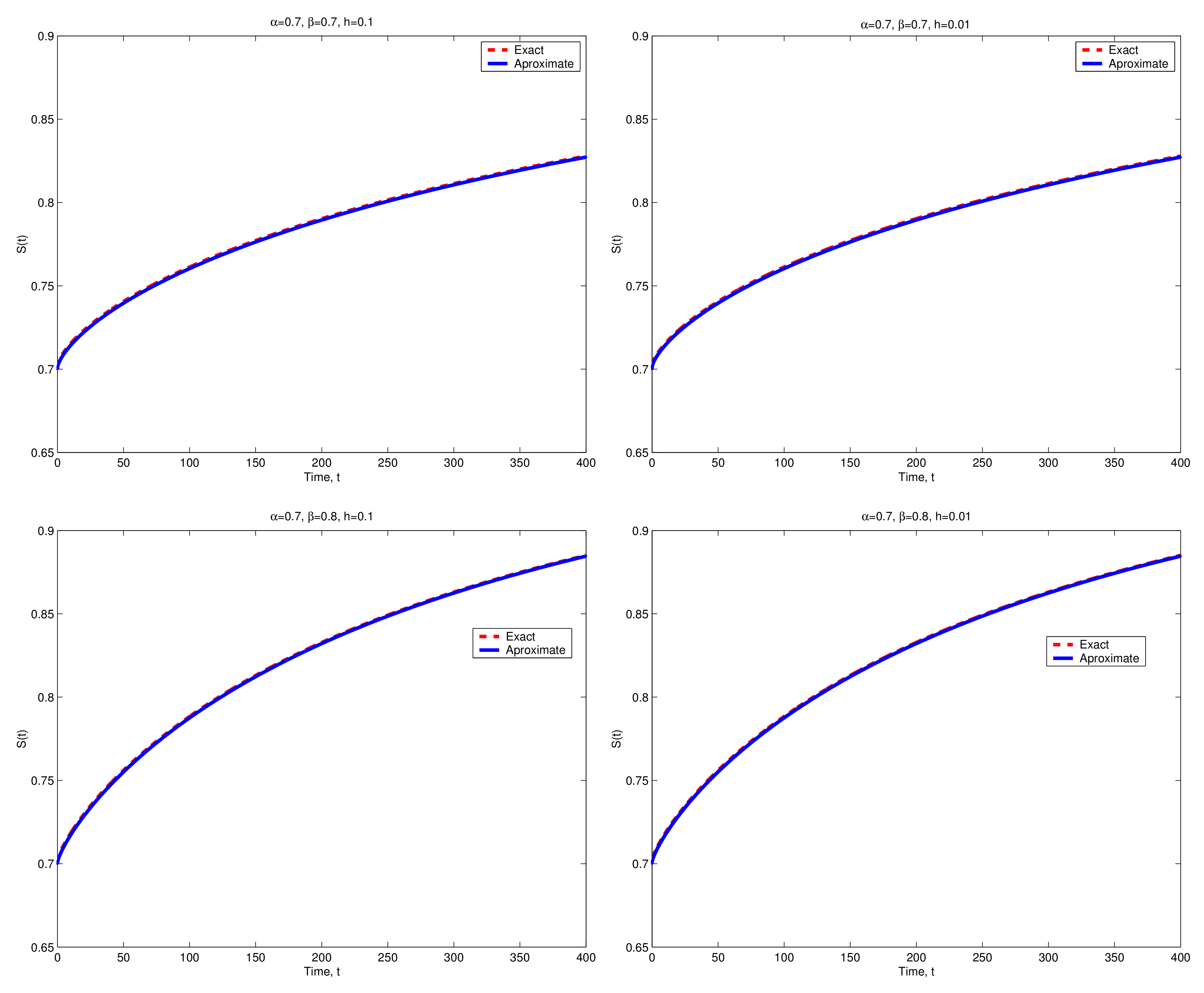
In the absence of disease, System (31) reduces to the following linear system:
From Lemma 2 of [28], the exact solution of (35) is given by
. Now, we apply the numerical scheme presented in (28) in order to approximate the solution of (35). For all numerical simulations, we chose , , and the normalization function as follows:
The comparison between the exact and numerical (approximate) solutions of (35) is displayed in Figure 1 for different values of , , and h.
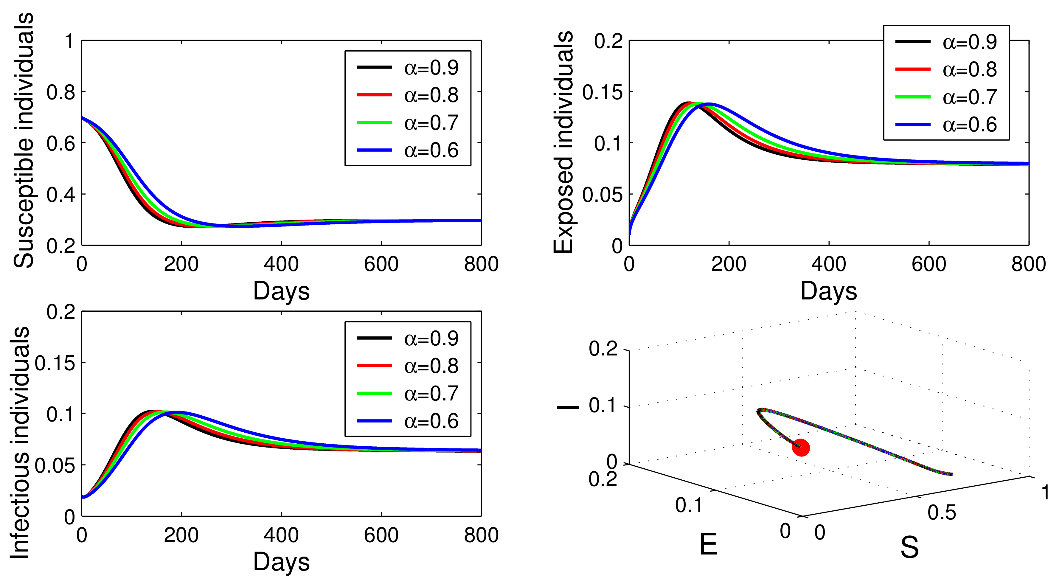
In the presence of disease, System (31) cannot be solved analytically. Based on our numerical method, we approximate the solution of (31). Therefore, we chose , , , and . By computation, we have . In this case, the solution of (31) converges to the endemic equilibrium , which biologically means that the disease persists in the population. Figure 2 illustrates this observation for different values of .
6. Conclusions
In this paper, we first investigated the qualitative properties of solutions of FDEs with the new generalized Hattaf fractional derivative, which includes several forms of fractional derivatives with non-singular kernels such as the Caputo–Fabrizio and Atangana–Baleanu fractional derivatives. In addition, we proposed a new numerical method to approximate the solutions of such types of FDEs. The obtained results extend and improve many results existing in the literature concerning the fractional comparison principle, stability, asymptotic stability, as well as Mittag–Leffler stability. Furthermore, the proposed numerical method includes the classical Euler numerical scheme, and it was applied to a nonlinear system describing the dynamics of an epidemic disease, such as COVID-19.
Funding
This research received no external funding.
Institutional Review Board Statement
Not applicable.
Informed Consent Statement
Not applicable.
Data Availability Statement
No data available.
Acknowledgments
The author would like to thank the anonymous reviewers for their constructive comments and suggestions, which have improved the quality of the manuscript.
Conflicts of Interest
The author declares no conflict of interest.
References
- Hattaf, K.; Yousfi, N. Global stability for fractional diffusion equations in biological systems. Complexity 2020, 2020, 5476842. [Google Scholar] [CrossRef]
- Magin, R.L. Fractional calculus models of complex dynamics in biological tissues. Comput. Math. Appl. 2010, 59, 1586–1593. [Google Scholar] [CrossRef] [Green Version]
- Cheneke, K.R.; Rao, K.P.; Edessa, G.K. Application of a new generalized fractional derivative and rank of control measures on Cholera transmission dynamics. Int. J. Math. Math. Sci. 2021, 2021, 2104051. [Google Scholar] [CrossRef]
- Qu, H.; Rahman, M.U.; Ahmad, S.; Riazd, M.B.; Ibrahim, M.; Saeed, T. Investigation of fractional order bacteria dependent disease with the effects of different contact rates. Chaos Solitons Fractals 2022, 159, 112169. [Google Scholar] [CrossRef]
- Zhang, L.; Rahman, M.U.; Ahmad, S.; Riaz, M.B.; Jarad, F. Dynamics of fractional order delay model of coronavirus disease. Aims Math. 2021, 7, 4211–4232. [Google Scholar] [CrossRef]
- Naji, F.A.; Al-Sharaa, I. Controllability of impulsive fractional nonlinear control system with Mittag–Leffler kernel in Banach space. Int. J. Nonlinear Anal. Appl. 2022, 13, 3257–3280. [Google Scholar]
- Meral, F.C.; Royston, T.J.; Magin, R.L. Fractional calculus in viscoelasticity: An experimental study. Commun. Nonlinear Sci. Numer. Simul. 2010, 15, 939–945. [Google Scholar] [CrossRef]
- Pinar, Z. On the explicit solutions of fractional Bagley-Torvik equation arises in engineering. Int. J. Optim. Control Theor. Appl. 2019, 9, 52–58. [Google Scholar] [CrossRef] [Green Version]
- Magin, R.L. Fractional Calculus in Bioengineering; Begell House: Danbury, CT, USA, 2006. [Google Scholar]
- Cao, X.; Lin, Y.-H.; Liu, H. Simultaneously recovering potentials and embedded obstacles for anisotropic fractional Schrödinger operators. Inverse Probl. Imaging 2019, 13, 197–210. [Google Scholar] [CrossRef] [Green Version]
- Cao, X.; Liu, H. Determining a fractional Helmholtz equation with unknown source and scattering potential. Commun. Math. Sci. 2019, 17, 1861–1876. [Google Scholar] [CrossRef]
- Lai, R.-Y.; Lin, Y.-H. Inverse problems for fractional semilinear elliptic equations. Nonlinear Anal. 2022, 216, 112699. [Google Scholar] [CrossRef]
- Srivastava, H.M.; Sahoo, S.K.; Mohammed, P.O.; Baleanu, D.; Kodamasingh, B. Hermite–Hadamard Type Inequalities for Interval-Valued Preinvex Functions via Fractional Integral Operators. Int. J. Comput. Intell. Syst. 2022, 15, 8. [Google Scholar] [CrossRef]
- Yang, S.; Liu, Y.; Liu, H.; Wang, C. Numerical methods for semilinear fractional diffusion equations with time delay. Adv. Appl. Math. Mech. 2022, 14, 56–78. [Google Scholar]
- Butt, A.I.K.; Ahmad, W.; Rafiq, M.; Baleanu, D. Numerical analysis of Atangana–Baleanu fractional model to understand the propagation of a novel corona virus pandemic. Alex. Eng. J. 2022, 61, 7007–7027. [Google Scholar] [CrossRef]
- Rahman, M.U.; Arfan, M.; Deebani, W.; Kumam, P.; Shah, Z. Analysis of time-fractional Kawahara equation under Mittag–Leffler Power Law. Fractals 2022, 30, 2240021. [Google Scholar] [CrossRef]
- Odabasi, M.; Pinar, Z.; Kocak, H. Analytical solutions of some nonlinear fractional-order differential equations by different methods. Math. Methods Appl. Sci. 2021, 44, 7526–7537. [Google Scholar] [CrossRef]
- Ashyralyev, A.; Dal, F.; Pinar, Z. A note on the fractional hyperbolic differential and difference equations. Appl. Math. Comput. 2011, 217, 4654–4664. [Google Scholar] [CrossRef]
- Ashyralyev, A.; Dal, F.; Pinar, Z. On the numerical solution of fractional hyperbolic partial differential equations. Math. Probl. Eng. 2009, 2009, 730465. [Google Scholar] [CrossRef]
- Li, Y.; Chen, Y.Q.; Podlubny, I. Stability of fractional-order nonlinear dynamic systems: Lyapunov direct method and generalized Mittag–Leffler stability. Comput. Math. Appl. 2010, 59, 1810–1821. [Google Scholar] [CrossRef] [Green Version]
- Podlubny, I. Mathematics in Science and Engineering. In Fractional Differential Equations; Academic Press: Cambridge, MA, USA, 1999; Volume 198. [Google Scholar]
- Delavari, H.; Baleanu, D.; Sadati, J. Stability analysis of Caputo fractional-order nonlinear systems revisited. Nonlinear Dyn. 2012, 67, 2433–2439. [Google Scholar] [CrossRef]
- Rao, M.R. Ordinary Differential Equations; East-West Press: Minneapolis, MN, USA, 1980. [Google Scholar]
- Slotine, J.J.E.; Li, W. Applied Nonlinear Control; Prentice Hall: Englewood Cliffs, NJ, USA, 1991. [Google Scholar]
- Kilbas, A.A.; Srivastava, H.M.; Trujillo, J.J. Theory and Applications of Fractional Differential Equations, North-Holland Mathematics Studies; Elsevier: Amsterdam, The Netherlands, 2006. [Google Scholar]
- Wang, G.; Pei, K.; Chen, Y.Q. Stability analysis of nonlinear Hadamard fractional differential system. J. Frankl. Inst. 2019, 356, 6538–6546. [Google Scholar] [CrossRef]
- Brzdek, J.; Eghbali, N.; Kalvandi, V. On Ulam stability of a generalized delayed differential equation of fractional order. Results Math. 2022, 77, 26. [Google Scholar] [CrossRef]
- Hattaf, K. Stability of fractional differential equations with new generalized Hattaf fractional derivative. Math. Probl. Eng. 2021, 2021, 8608447. [Google Scholar] [CrossRef]
- Hattaf, K. A new generalized definition of fractional derivative with non-singular kernel. Computation 2020, 8, 49. [Google Scholar] [CrossRef]
- Caputo, A.; Fabrizio, M. A new definition of fractional derivative without singular kernel. Prog. Fract. Differ. Appl. 2015, 1, 73–85. [Google Scholar]
- Atangana, A.; Baleanu, D. New fractional derivatives with non-local and non-singular kernel: Theory and application to heat transfer model. Therm. Sci. 2016, 20, 763–769. [Google Scholar] [CrossRef] [Green Version]
- Al-Refai, M. On weighted Atangana–Baleanu fractional operators. Adv. Differ. Equ. 2020, 2020, 3. [Google Scholar] [CrossRef] [Green Version]
- Hattaf, K.; Mohsen, A.A.; Al-Husseiny, H.F. Gronwall inequality and existence of solutions for differential equations with generalized Hattaf fractional derivative. Math. Comput. Sci. 2022, 27, 18–27. [Google Scholar] [CrossRef]
- Hattaf, K. On some properties of the new generalized fractional derivative with non-singular kernel. Math. Probl. Eng. 2021, 2021, 1580396. [Google Scholar] [CrossRef]
- Djida, J.D.; Atangana, A.; Area, I. Numerical Computation of a Fractional Derivative with Non-Local and Non-Singular Kernel. Math. Model. Nat. Phenom. 2017, 12, 4–13. [Google Scholar] [CrossRef] [Green Version]
- Baleanu, D.; Fernandez, A. On some new properties of fractional derivatives with Mittag–Leffler kernel. Commun. Nonlinear Sci. Numer. Simul. 2018, 59, 444–462. [Google Scholar] [CrossRef] [Green Version]
- Zhang, F.; Li, C.; Chen, Y.Q. Asymptotical stability of nonlinear fractional differential system with Caputo derivative. Int. J. Differ. Equ. 2011, 2011, 635165. [Google Scholar] [CrossRef]
Figure 1.
The exact and numerical solutions of (35) for different values of , , and h.

Figure 2.
The numerical solution of (31) for different values of .


Table 1.
Biological meanings of the parameters of model (30).
| Parameter | Biological Meaning |
|---|---|
| A | Natality or recruitment rate |
| Natural death rate | |
| Transmission rate of disease | |
| Transfer rate from class E to class I | |
| r | Recovery rate of the infectious individuals |
Publisher’s Note: MDPI stays neutral with regard to jurisdictional claims in published maps and institutional affiliations. |
© 2022 by the author. Licensee MDPI, Basel, Switzerland. This article is an open access article distributed under the terms and conditions of the Creative Commons Attribution (CC BY) license (https://creativecommons.org/licenses/by/4.0/).
Share and Cite
MDPI and ACS Style
Hattaf, K. On the Stability and Numerical Scheme of Fractional Differential Equations with Application to Biology. Computation 2022, 10, 97. https://0-doi-org.brum.beds.ac.uk/10.3390/computation10060097
AMA Style
Hattaf K. On the Stability and Numerical Scheme of Fractional Differential Equations with Application to Biology. Computation. 2022; 10(6):97. https://0-doi-org.brum.beds.ac.uk/10.3390/computation10060097
Chicago/Turabian StyleHattaf, Khalid. 2022. "On the Stability and Numerical Scheme of Fractional Differential Equations with Application to Biology" Computation 10, no. 6: 97. https://0-doi-org.brum.beds.ac.uk/10.3390/computation10060097
Note that from the first issue of 2016, this journal uses article numbers instead of page numbers. See further details here.