
An Experimental Study on Speech Enhancement Based on a Combination of Wavelets and Deep Learning


Electrical Engineering Department, University of Costa Rica, San José 11501-2060, Costa Rica
*
Author to whom correspondence should be addressed.
†
These authors contributed equally to this work.
Computation 2022, 10(6), 102; https://0-doi-org.brum.beds.ac.uk/10.3390/computation10060102
Submission received: 29 April 2022
/
Revised: 11 June 2022
/
Accepted: 16 June 2022
/
Published: 20 June 2022
(This article belongs to the Special Issue Bioinspiration: The Path from Engineering to Nature)
Abstract
:The purpose of speech enhancement is to improve the quality of speech signals degraded by noise, reverberation, or other artifacts that can affect the intelligibility, automatic recognition, or other attributes involved in speech technologies and telecommunications, among others. In such applications, it is essential to provide methods to enhance the signals to allow the understanding of the messages or adequate processing of the speech. For this purpose, during the past few decades, several techniques have been proposed and implemented for the abundance of possible conditions and applications. Recently, those methods based on deep learning seem to outperform previous proposals even on real-time processing. Among the new explorations found in the literature, the hybrid approaches have been presented as a possibility to extend the capacity of individual methods, and therefore increase their capacity for the applications. In this paper, we evaluate a hybrid approach that combines both deep learning and wavelet transformation. The extensive experimentation performed to select the proper wavelets and the training of neural networks allowed us to assess whether the hybrid approach is of benefit or not for the speech enhancement task under several types and levels of noise, providing relevant information for future implementations.
1. Introduction
Voice is the most common and effective form of communication between persons. Since the early years of human kind, persons have exchanged thoughts, indications, and in general information using our voices. From the perspective of analysis and processing this information using technology, the voice is a sound signal, which will be disturbed by noises when it is propagated in living environments [1].
The enhancement of these signals affected by noise has a long history among the researchers in signal processing and remains a challenging problem under a variety of dynamic scenarios and several types of noises and levels. The purpose of the various techniques developed to deal with the noise that contaminates the speech sounds is to remove the noise as much as possible, so users or systems can receive the original speech signal after removing the noise without sacrificing the intelligibility and clarity of the speech.
This process of enhancing is of great importance for many applications, such as mobile phone communications, VoIP, teleconferencing systems, hearing aids, and automatic speech recognition (ASR) systems. For example, several authors have reported a decrease in the performance of ASR in the presence of noise recently [2,3,4], and there is concern about the performance of devices for hearing aids as well [5,6].
In order to overcome this relevant problem, a number of algorithms have been presented in the literature (reviews on this topic can be consulted in [7,8]). According to such reviews and previous references [9,10], those algorithms can be divided into two basic categories: Single-Channel Enhancing Techniques and Multi-Channel Enhancing Techniques.
From the first category, two main approaches have been presented:
- a
- Spectral Subtraction Method, which uses estimations of statistics of the signal and the noise. It is suitable for real-time applications due to its simplicity. The first assumption is that the speech and the noise can be modeled using an addition of the single component:where is the clean speech signal and the noise signal. In the frequency domain, this expression can be written asThe estimation of the enhanced speech can be expressed asThe enhanced signal can be obtained in the time domain using the inverse Fourier transform in Equation (3) with the phase information.
- b
- Spectral Subtraction with Over-subtraction Model (SSOM):The previous method applies a difference in the spectral domain based on a statistical average of the noise. If such a statistical average is not representative of the signal, for example, in musical background noise, in this case, a value floor of minimum spectrum values is established, which leads to minimizing the narrow spectral peaks by decreasing the spectral excursions.
- c
- Non-Linear Spectral Subtraction: This method is based on a combination of the two previous algorithms, considering the subtraction based on the signal-to-noise ratio (SNR) of each frame. That makes the process nonlinear, applying less subtraction where the noise is less present, and vice versa.
The limitation of these spectral subtraction methods were addressed previously in [11].
For the second class of algorithms, the systems take advantage of available multiple signal inputs in separate channels and perform significantly better for non-stationary noises. The main algorithms are:
- a
- Adaptive Noise Cancellation: This method takes advantage of the principle of destructive interference between wave sounds, by using a reference signal to generate an anti-noise wave of equal amplitude, but opposite phase. Several strategies have been applied for defining this reference signal, for example using sensors located near the noise and interference sources.
- b
- Multisensor Beamforming: This method is applicable when the sound is recorded using a geometric array of microphones. The sound signals are amplified or attenuated (in the time or frequency domain) depending on their direction of arrival. The phase information is particularly important, because most methods reject all the noisy components not aligned in phase.
Other authors, such as [9], have presented complementary categories of speech enhancement algorithms, including statistical-model-based algorithms, where measurements of noisy segments of recordings are used to estimate the parameters of the clean speech from the segments where both signals are present. Another relevant category would be the subspace algorithms based on the principle of applying linear algebra theory: the speech signals can be mapped to a different subspace than the noise subspace.
With the recent developments in deep learning, based on complex models of artificial neural networks, the process of learning a mapping function between noise-corrupted speech to clean speech has been applied successfully. In this domain, artificial neural networks can be defined as a class of machine learning models initially intended to imitate some characteristics of the human brain by connecting units organized in layers, which propagate information through internal connections. Clean speech parameters can be predicted from noisy parameters by combining complex neural network architectures and deep learning procedures, as presented in [12,13,14].
In most cases, the application of deep neural networks has surpassed the results of other algorithms previously presented in the literature and, thus, can be considered the state-of-the-art in speech denoising for several noisy conditions.
On the other hand, wavelet denoising, which considers a different approach than the mapping function, has also been presented in the literature for the task of removing noise in speech signals recently, even with noise collected from real environments [15]. From these considerations, in this work, we study the combination of the wavelet and deep learning denoising approaches in a hybrid implementation, where both algorithms process the noisy signals to enhance their quality. The idea of combining algorithms in a cascade approach has been presented previously, but with a combination of deep learning and classical signal-processing-based algorithms. To our knowledge, this is the first extended study on the combination of Long Short-Term Memory neural networks and wavelet transforms.
The results of this experimental study can benefit current and future implementation of speech enhancement, in systems such as videoconferencing and audio restoration, where the improvement in the quality of the speech is imperative, and therefore the selection of the simple or hybrid approaches can be performed carefully. Furthermore, the hybrid methodology results can establish a baseline for future proposals on a new combination of enhancement algorithms.
1.1. Related Work
This section focuses on the hybrid approaches to speech denoising and previous experiences with wavelet transform presented in the literature. The application of deep neural networks as an isolated algorithm for this purpose has been reported in a number of publications and reviewed recently in [16,17].
The wavelet-denoising-based references usually specify the problem of the threshold in the wavelet functions and measuring the signal-to-noise ratio before and after the application of the functions. For example, in a recent report presented in [1], four threshold selection methods were applied, using sym4 and db8 wavelets. Some authors provide experimental validation for different noisy signals and proved that the denoising method of the speech signal based on wavelet analysis is effective in enhancing noisy speech signals.
A two-stage wavelet approach was developed in [18], first by estimating the speech presence probability and, then, removing the coefficients of the noise floor. Results in speech degraded with Pink and White noise from a signal-to-noise ratio of 0 to a signal-to-noise ratio of -8 surpassed several classical algorithms.
A hybrid of deep learning and the vector Wiener filter was presented recently in [19], showing benefits from the combined application of algorithms. Other than the deep-learning-based hybrid approach, contemplating harmonic regeneration noise reduction and a comb filter was reported in [20] and validated using also subjective measurements. Another two-stage estimation algorithm based on wavelets was proposed in [21], as a previous stage to more traditional algorithms such as the Wiener filter and MMSE.
One implementation of the wavelet transform for enhancing noisy signals in ranges of the SNR from −10 to SNR 10, with a great variety of natural and artificial noises, was presented in [22]. The success of the proposal was observed especially for lower SNR levels.
Hybrid approaches that combine wavelets and other techniques for speech enhancement are also part of the proposals presented in the literature. For example, a combination of wavelets and a modified version of principal component analysis (PCA) was presented in [23]. The results showed relevant noise reduction for several kinds of artificial and natural noises and a lower signal distortion without introducing artifacts.
In terms of wavelets and deep learning hybrid approaches, some recent experiences were explored in [24], by applying the wavelet transform for the decomposition of the signal and in a second stage, the radial basis function network (RFBN). The performance of the proposal was described as excellent by the authors, using objective measures such as the segmental signal-to-noise ratio (SegSNR) and PESQ.
1.2. Problem Statement
The purpose of speech enhancement of a noisy signal is to estimate the uncorrupted speech signal from the degraded speech signal. Several speech denoising algorithms estimate the characteristics of the noise from silent segments in the speech utterances or by mapping the signal into new domains, such as with the wavelet transform.
In our case, we considered segments of noisy and clean speech to compare the enhancement using wavelets, deep learning, and both methods in cascade. As stated in [25], the enhancing process using wavelets can be summarized as follows: Given and , the forward and inverse wavelet transform operators, and , the denoising operator with threshold , the process is performed using the three steps:
- Transform using a wavelet: .
- Obtain the denoised version using the threshold, in the wavelet domain: .
- Transform the denoised version into the time domain: .
On the other hand, the enhancement using artificial neural networks is performed by learning a mapping function f between the spectrum of and with the criteria
f is approximated using a Recurrent Neural Network, which outputs a version of the denoised signal after the training process.
In the hybrid approach, the first step of wavelet denoising provides to the neural networks, which is trained with the criteria
with the purpose of obtaining , a better approximation of than and .
2. Materials and Methods
In this section, the main techniques and procedures to establish the Experimental Setup to evaluate the proposed Hybrid approach are presented.
2.1. Wavelets
Wavelets are a class of functions that have been successfully applied in the discrimination of data from noise data, emulating a filter. The wavelet transform uses an infinite set of functions of different scales and at different locations to map a signal into a new domain, the wavelet domain [26].
It has become an alternative to the Fourier transform and can be related to similar families of function transformations, but with a particular interest in the scale or resolution of the signals.
In the continuous-time domain, a wavelet transform of a function is defined as [25]:
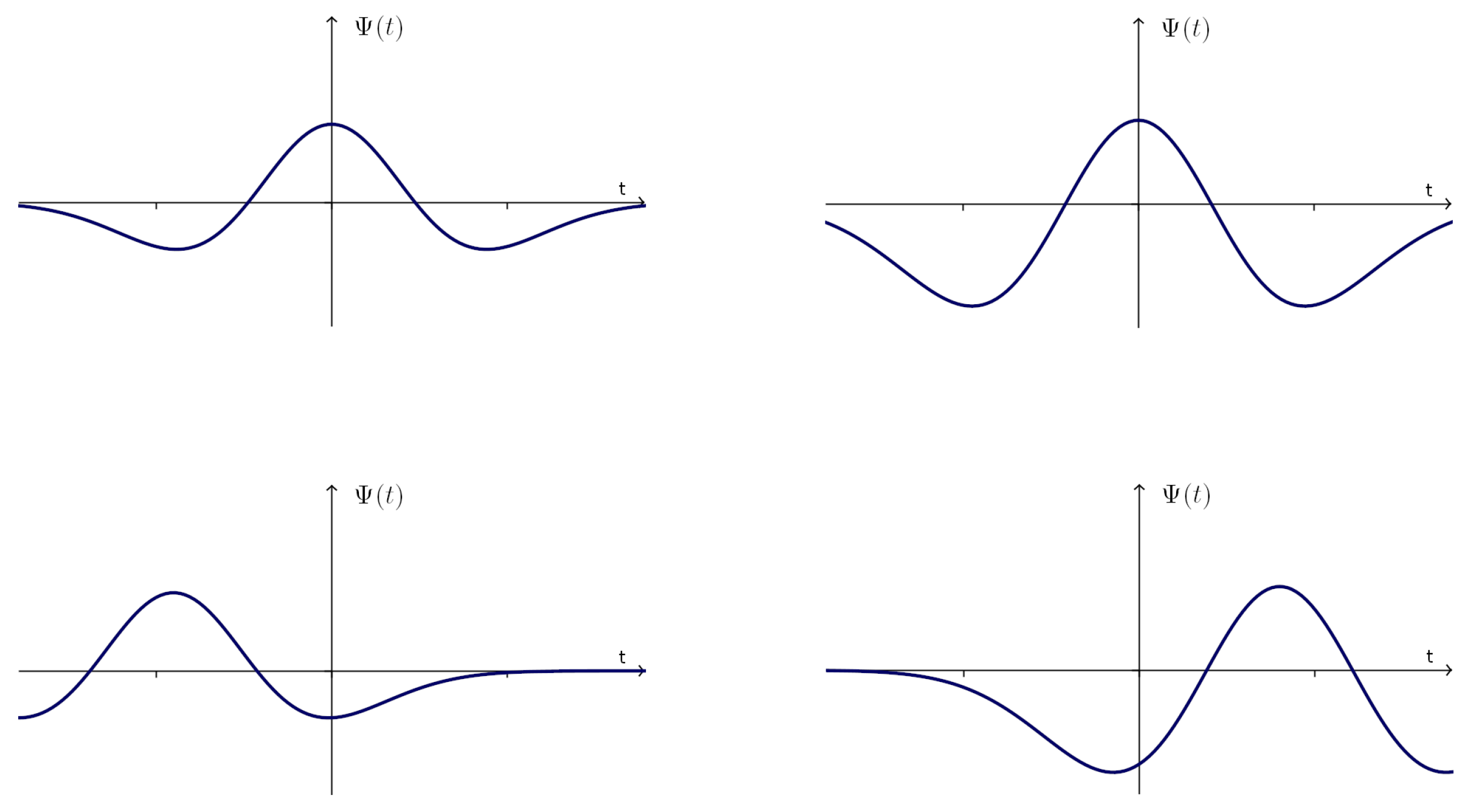
where and are real numbers that represent dilating and translating coefficients. The function is called the mother wavelet and requires the property of having a zero net area. There is a variety of mother wavelet functions, for example: Haar, Symlet, and Ricker, among many others. Different values of a and b provide variants of scales and shifts of the mother wavelet, as shown in Figure 1.
The fundamental idea behind wavelets is to analyze the functions according to the scale [27], representing them as a combination of time-shifted and scaled representations of the mother wavelet. For the selection of the best mother wavelet for a particular application, an experimental approach needs to be implemented [28]. For example, in the case of electroencephalogram (EEG) signals, more than forty mother functions were tested in [29], to determine the Symlet wavelet of order nine as the best option for that problem.
The wavelet transform provides coefficients related to the similarity of the signal with the mother function. A detailed mathematical description of wavelets can be found in [30,31,32].
The application of wavelets for denoising signals using thresholding emerged in the 1990s from the works [33,34]. The threshold can be of two types: soft thresholding and hard thresholding, and the idea is to reduce the magnitude or completely remove the coefficients in the wavelet domain.
The process of denoising using this approach can be described using the following steps [35]:
- Apply the wavelet transform to the noisy signal, to obtain the wavelet coefficients.
- Apply the thresholding function and procedure to obtain new wavelet coefficients.
- Reconstruct the signal by inverse transforming the coefficients after the threshold.
According to [36], wavelet denoising gives good results in enhancing noisy speech for the case of White Gaussian noise. Wavelet denoising is considered a non-parametric method. The choice of the mother wavelet function determines the final waveform shape and has an important role in the quality of the denoising process.
2.1.1. Thresholding
The threshold process affects the magnitude or the amount of coefficients in the wavelet domain. The two most popular approaches are hard thresholding and the soft thresholding. In the first type, hard thresholding, the coefficients whose absolute values are lower than , are set to zero. The soft thresholding performs a similar operation, but also shrinks the nonzero coefficients. This operation can be mathematically described as sign if and is 0 if [25]. The two types of thresholding are illustrated in Figure 2.
To implement the thresholds, several estimation methods are available in the literature. Four of the well-known standard threshold estimation methods are [37,38]:
- Minimax criterion: In statistics, the estimators face the problem of estimating a deterministic parameter from observations. The minimax method minimizes the cost of the estimator in the worst case. For the case of threshold selection, the principle is applied by assimilating the de-noised signal to the estimator of the unknown regression function. This way, the threshold can be expressed as:where and is the wavelet coefficient vector of length N.
- Sqtwolog criterion: The threshold is calculated using the equationwhere is the median absolute deviation (MAD) and is the length of the noisy signal at the scale.
- Rigrsure: The soft threshold can be expressed aswhere is the squared wavelet coefficient chosen from a vector consisting of the squared values of the wavelet coefficients and is the standard deviation.
- Hersure: The threshold combines Sqtwolog and Rigrsure, given the property that the Rigrsure threshold does not perform well at a low SNR. In such a case, the Sqtwolog method gives better threshold estimation. If the estimation from Sqtwolog is and from Rigrsure is , then Hersure uses:where, given the length of the wavelet coefficient N and s, the sum of squared wavelet coefficients, the values of A and B are calculated as
2.1.2. No Thresholding Alternative
Research on the implementation of wavelet denoising without using a threshold can be found in [39,40]. This approach considers using a functional analysis method based on the entropy of the signal, and this algorithm takes advantage of a constructive structural property of the wavelet tree with respect to a defined seminorm; it consists of searching for minima for the low-frequency domain and other minima for the high-frequency domain.
2.2. Deep Learning
Deep learning is a subset of machine learning techniques that allows computers to process information in terms of a hierarchy of concepts [41]. Typically, deep learning is based on artificial neural networks, which are known for their capacity as universal function approximations with good properties of self-learning, adaptivity, and advancement in input to an output mapping [42]. With this capacity, computers can learn complex operations and functions by building them out of simpler ones.
Previous to the development of deep learning techniques and algorithms, other approaches were almost unable to process natural data in their raw form. For this reason, the application of pattern-recognition or machine-learning systems required domain expertise to understand the problems, obtain the best descriptors, and apply the techniques using feature vectors that encompass the descriptors [43].
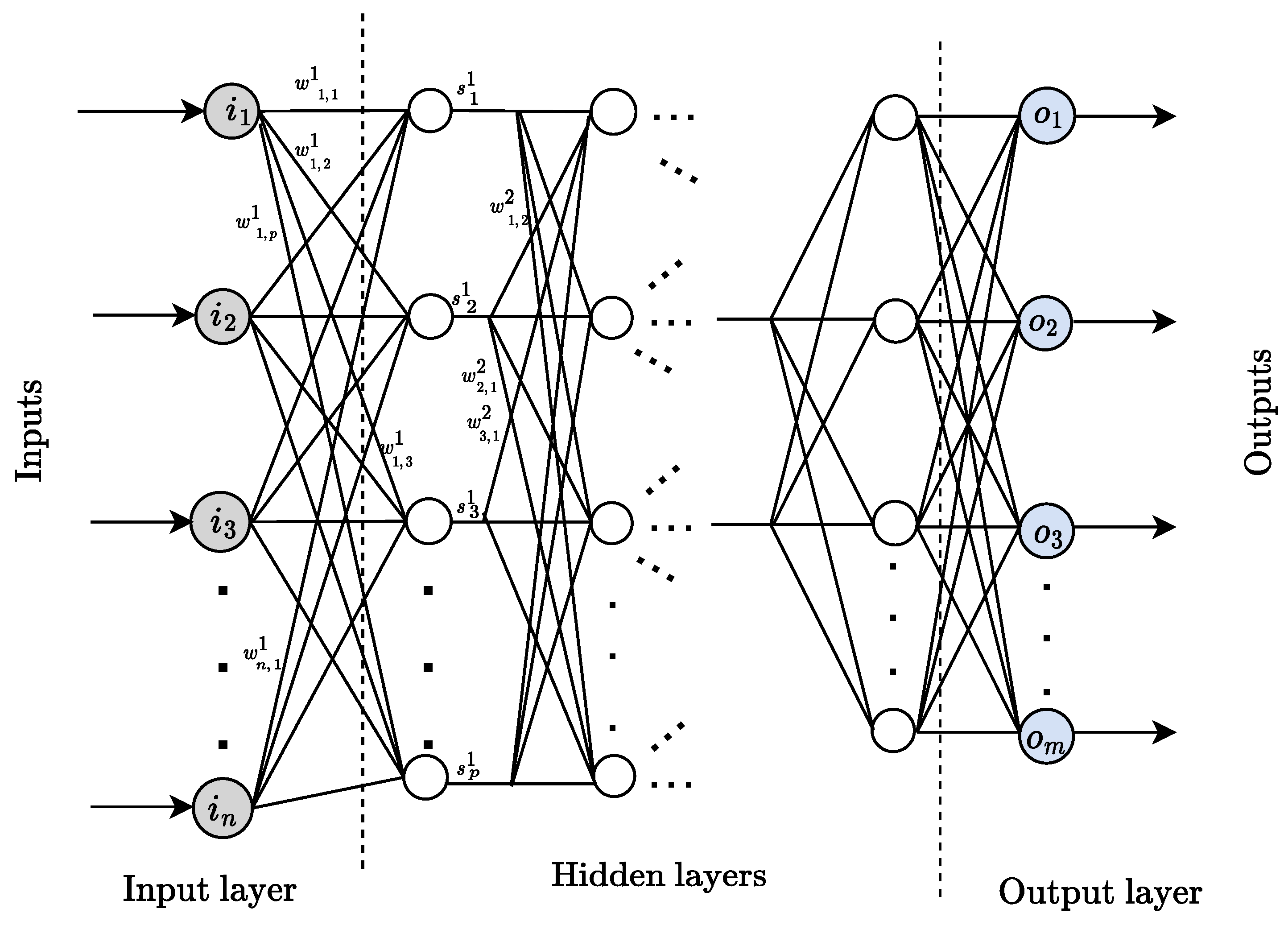
The most common form of deep learning is by composing layers of neural network units. The first level receives the data (in some cases, raw data), and subsequent layers perform other transformations. After several layers of this process, significantly complex functions can be learned. The feedforward deep neural network, or multi-layer perceptron (MLP) with more than three hidden layers, is a typical example of a deep learning algorithm. The architecture of a MLP organized with multiple units, inputs, outputs, and weights can be represented graphically [44], as shown in Figure 3.
Each layer performs a function from the inputs (or the outputs of the previous layer) to the outputs, using activation functions defined in each unit and the value of the weight of the connections. For example, a network with three layers defines functions ,, , and this way, the whole network performs a function from inputs x to the outputs defined as [41].
The purpose of the training process of a deep neural network is to approximate some mapping function , where x are inputs and the networks’ parameters, such as the value of the connections between units and the hyperparameters of learning (e.g., the learning rate and the bias). One of the most relevant aspects of deep learning is that the parameter is learned from data using a general-purpose learning procedure [43]. This way, deep learning has shown its capability to solve problems that have resisted previous attempts in the artificial intelligence community.
The success of deep learning in speech recognition and image classification in 2012 is often cited as the leading result of the renaissance of deep learning, using architectures and approaches such as deep feedforward neural networks, convolutional neural networks (CNNs), and Long Short-Term Memory (LSTM) [45].
One of the most important architectures of deep neural networks applied to signal processing is autoencoders. Autoencoders are designed to reconstruct or denoise input signals. For this reason, the output presents the same dimensionality as the inputs. Thus, autoencoders consist of encoding layers and decoding layers. The first stage removes redundant information in the input, while decoding layers reverse the process [17]. With the proper training, pairs of noisy/clean parameters can be presented to the autoencoder, and the approximation function gives denoising properties to the network.
A massive amount of data are often required, given the huge amount of parameters and hyperparameters of autoencoders and the deep networks in general. Furthermore, the recent advances in machine parallelism, such as cloud computing and GPUs, are of great importance to perform the training procedures in a short time [45].
From this experience, we selected the recent implementation of the stacked dual-signal transformation LSTM network (DTLN). This implementation combines a short-time Fourier transform (STFT) and a pre-trained stacked network. This combination enables the DTLN approach to extract information from magnitude spectra and incorporate phase information, providing state-of-the-art performance.
The DTLN has 128 units in each of its LSTM layers. The networks’ inputs correspond to information extracted from a frame size of 32 ms and a shift of 8 ms, using an FFT of size 512. An internal convolutional layer with 256 filters to create the learned feature representation is also included. During training, 25% of dropout is implemented between the LSTM layers. The optimization algorithm applied to update the network weights was Adam, first presented in [46], using a learning rate of . This implementation is capable of real-time processing, showing state-of-the-art performance. Its architecture combines LSTM, dropout, and convolutional layers, resulting in a total of 986753 trainable parameters. Further details of the implementation can be found in [47].
2.3. Proposed System
In order to test our proposal, the first step is to generate a dataset of noisy speech with both natural and artificial noise at several signal-to-noise ratio levels. This procedure establishes parallel data of clean and noisy speech and allows the comparison of speech quality before and after the application of the denoising procedures.
Our focus is on the combination of wavelet-based and deep-learning-based speech denoising, with the purpose of comparing the performance of both separately and analyzing the suitability of both in a two-stage approach. In the case of wavelet-based denoising, the following four steps were applied in an extensive experimentation, according to the description presented in Section 2.1:
- Select a suitable mother wavelet.
- Transform each speech signal using the mother wavelet.
- Select the appropriate threshold to remove the noise.
- Apply the inverse wavelet transform to obtain the denoised signal.
There is a variety of criteria that can be used to choose the mother wavelet, such as the ones presented in [27,48]. In our case, an experimental approach was implemented, following a process of trial and error with commonly used wavelet families for speech denoising such as Daubechies, Symlet, and biorthogonal.Different wavelets from each family (using common ranges) were tested using objective measures, and the wavelets with the best results in each case were tested again; finally, the wavelet with the best results among the wavelet families was selected. This process was made using the Wavelet-Denoiser System (https://github.com/actonDev/wavelet-denoiser, accessed on 28 April 2022) to determine the best combination of mother wavelets and parameters for each case.
For the application of the deep-learning-based denoising, the procedure can be summarized in the following steps:
- Select one architecture of the network: In our experiments, we used the stacked dual-signal transformation LSTM network architecture presented in [47]. The architecture was based on two LSTM layers followed by a fully connected (FC) layer.
- Train the deep neural network with pairs of noisy and clean speech at the inputs and at the outputs. For the case of the hybrid approach, the outputs of the wavelet denoising were used as the inputs of the neural network, which were re-trained completely using pairs of wavelet-based denoising and clear speech.
- Establish a stop criterion for the training procedure.
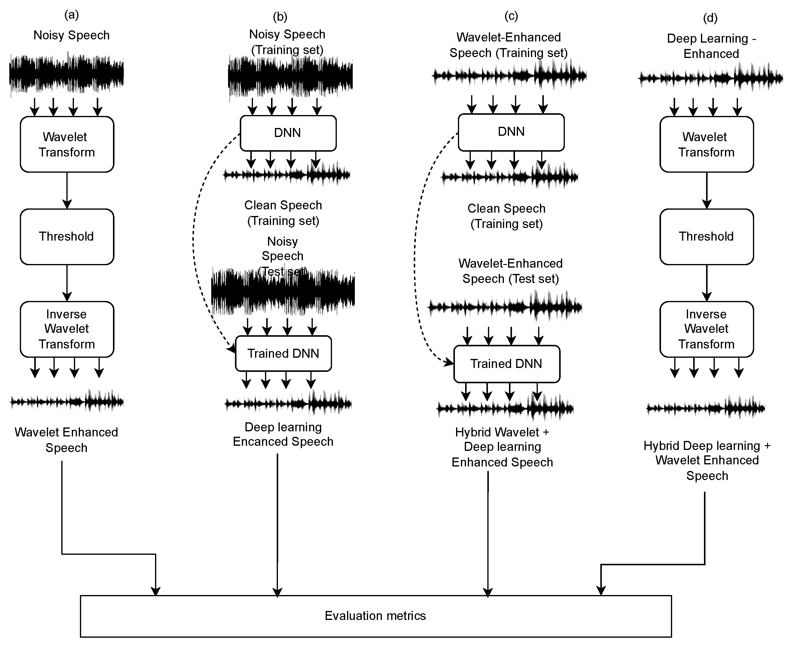
As in the case of wavelets, objective measures can be applied to validate the benefits of the deep neural networks in each noise type and level. With the purpose of performing a proper comparison, the same amount of epochs for training the deep neural networks was used for both (noisy, clean) and (wavelet-denoised, clean) procedures. Additionally, for the sake of completeness in the experiments, we also considered a two-stage approach with the application of wavelet denoising to the results of the deep-learning-based denoising procedure. This experimental approach can be summarized in four possibilities to implement and compare, as illustrated in Figure 4.
2.4. Experimental Setup
In this section, a detailed description of the data and the evaluation process is presented.
2.4.1. Dataset
In order to test our hybrid proposal based on wavelets and deep learning, we chose the CMU ARCTIC databases, constructed at the Language Technologies Institute at Carnegie Mellon University. The recordings and their transcriptions are freely available in [49]. The dataset consists of more than 1100 recorded sentences, selected from Project Gutenberg’s copyright-free texts. The recordings were sampled at 16KHz in WAV format.
Four native English speakers recorded each sentence, and their corresponding files were labeled as bdl (male), slt (female), clb (female), and rms (male). For our experiments, we chose the slt voice and defined the training, validation, and test sets according to the common criteria of the data available: 70%, 20%, and 10%, respectively. The randomly selected utterances that conform the test set for the deep neural networks were shared in the evaluation of the four cases described in Section 2.3.
2.4.2. Noise
To compare the capacity of the four cases contemplated in our proposal, the database was degraded with additive noise of three types: two artificially generated noises (White, Pink) and one natural noise (Babble). To cover a wide range of conditions, five levels of signal-to-noise (SNR) ratios were considered for each case. This gives the following dataset:
The whole set of voices to compare can be listed as:
- Clean, as the dataset described in the previous section.
- The same dataset degraded with additive White noise added at five SNR levels: SNR −10, SNR −5, SNR 0, SNR 5, and SNR 10.
- The clean dataset degraded with additive Pink noise added at five SNR levels: SNR −10, SNR −5, SNR 0, SNR 5, and SNR 10.
- The clean dataset degraded with additive Babble noise added at five SNR levels: SNR −10, SNR −5, SNR 0, SNR 5, and SNR 10.
2.4.3. Evaluation
The evaluation metrics defined for our experiments were based on measures commonly applied in noise reduction and speech enhancement, namely, perceptual evaluation of speech quality (PESQ), and frequency domain segmental signal-to-noise ratio (SegSNR).
The first measure is based on a psychoacoustic model to predict the subjective quality of speech, according to ITU-T recommendation P.862.ITU. Results are given in interval , where 4.5 corresponds to a perfect signal reconstruction [50,51].
The second measure is frame-based, calculated by averaging the SNR estimates at each frame, using the equation:
where is Fourier transform coefficient of frame i and is the coefficient for the processed speech. N is the number of frames and L the number of frequency bins. The values of this measure are given in the interval dB.
Additionally, we present waveforms and spectrogram visual inspection to illustrate the result of the different approaches.
3. Results and Discussion
In this study, five SNR levels, three types of noise, and two objective measurements were explored to evaluate the performance of the four different algorithms described in Section 2.3. A sample visualization of the different waveforms involved in the study is shown in Figure 5.
The objective measures of PESQ and SegSNR are reported as the mean of fifty measures calculated on the test set. To select the mother wavelet and the threshold, extensive experimentation was conducted. For every case reported in the results, more than twenty possibilities were tested. The most successful mother wavelets were db1 and db2.
For the deep learning and hybrid approaches involving neural networks, the stop criterion was defined as the number of epochs. The same number of epochs used for the training of the networks from the noisy to clean signal were replicated in the hybrid proposals, for the sake of comparison.
The results for the PESQ measure and the Babble noise degradation and filtering are presented in Table 1. A first relevant result can be observed on the small benefit that was measured for the case of the wavelet enhancement. A better performance than those of the wavelets was obtained with the deep learning enhancement for every SNR level of Babble noise. In terms of the hybrid combination of wavelets and deep learning, the deep neural networks as a second stage achieved an improvement in three of the five cases of PESQ. Furthermore, an increase on SegSNR was measured in two of the five cases with the same hybrid combination, as presented in Table 2.
For all the cases of the SegSNR measure with Babble noise, it was observed that the wavelet transform did not represent significant improvements of the results. This can explain why none of the hybrid approaches performed better than deep learning alone, with the exception of two cases.
The benefits of the hybrid approaches were consistently better for the case of Pink noise. The results for PESQ and the different levels of this type of noise are presented in Table 3. For this measure, the hybrid approach of wavelets + deep learning gave better results in four of the five noise levels. This results are important because the application of wavelets did not improve any of the cases in terms of the SNR, but, as shown in Table 4, an increase in SegSNR was consistent.
Such results can be interpreted in terms of improvements incorporated into the signals with the application of wavelets, which did not improve the perceptual quality of the speech sounds, but the mapping of the noisy signals into a different version is beneficial for the enhancement using deep learning.
The best results of the hybrid approach of wavelets + deep learning were obtained for the case of White noise. Table 5 shows the results of the PESQ measure. For all the noise SNR levels, such a hybrid approach gave the best results, even when the first stage of wavelet enhancement did not improve the quality of the signal. However, in a similar way to the previous case, Table 6 shows how the wavelets improved the SegSNR in all the cases of White noise degradation.
The improvements on the SegSNR measure with the hybrid approach were consistent also at all SNR levels of White noise. For this case, it is also significant that the hybrid combination of deep learning and wavelets as a second stage also surpassed the results of deep learning.
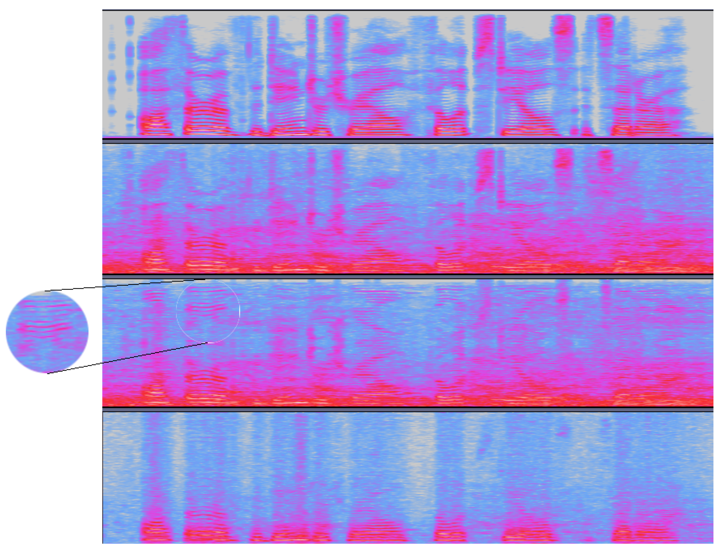
For all types of noise, the application of wavelets as the second stage of enhancement did not represent any relevant benefit in terms of PESQ, in comparison to the deep learning approach. From a visual inspection of the spectrograms in Figure 6, it seems that the application of wavelets introduced some patterns at the higher frequencies and blurred some relevant information at those bands as well.
This kind of result may explain also why wavelets did not improve significantly the PESQ of the noisy utterances, but helped to improve the SegSNR (in particular in the case of White noise). Especially for the case of White noise, the wavelets as an intermediate representation of the signals seemed to represent advantages for the application of the deep learning enhancement.
The results of this work may represent similar benefits to recent proposals of combining wavelets and deep learning, for example, in [52], where deep learning performed the mapping in the wavelet domain. In our case, deep learning was applied as a second stage of enhancement (and as a first stage prior to wavelets). In that work, relevant benefits in terms of improving the SNR were found.
Other hybrid or cascade approaches have been tested recently in similar domains, for example, speech emotion recognition [53]. The results of this study may represent an opportunity to develop more hybrid approaches, where the benefit of each stage can be analyzed separately, in a similar way to image enhancement, where different algorithms to enhance aspects such as noise, blur, and compression have been applied separately, using a cascade approach.
4. Conclusions
In this paper, we analyzed the hybrid combination of wavelets and deep learning for the enhancement of speech signals. For this purpose, we conducted an extensive experimentation for the selection of parameters of the wavelet transform and the training of more than forty deep neural networks to measure whether or not the combination of both deep learning and wavelets (as both the first or second stages) benefits the enhancement of speech signals degraded with several kinds of noise. To establish a proper comparison, some restrictions were introduced in the experimentation, such as the limitation of epochs during training to match the hybrid and deep learning cases.
The results showed benefits of the hybrid application of first wavelet enhancement and deep learning as a second stage, especially for the case of White noise. Those benefits were measured in comparison to the noisy signal and the enhancement with wavelets and deep learning alone. For other types of noise, in particular Babble, the hybrid approach presented mixed results, with benefits on some of the SNR levels analyzed. This type of noise, which is more complex and irregular than the synthetic White and Pink noises, was the most challenging scenario of those contemplated in this work. The application of deep learning as a unique stage presents better results for that case. For the case of Pink noise, the hybrid approach enhancement shows better results than the separate algorithms for the higher levels of noise. When the SNR was as low as 5 or 10, deep learning performed better.
The wavelet denoising succeed in enhancing the signals in terms of SegSNR (except for Babble noise, where the benefits were almost null), but some artifacts observed in the spectrograms may explain why its benefits were not measurable in terms of PESQ. Regardless, the output obtained with the wavelet enhancement represents a better input to the deep neural networks than the noisy signals. The benefits of applying a combination of deep learning and other algorithms are present in the scientific literature, and future works may define the particular benefits of the separate algorithms in order to establish optimized hybrid applications for particular noise types and levels.
Several research opportunities can follow the results of this study. For example, an analysis of delays in real-time applications using the hybrid proposal could be addressed in order to establish the feasibility of implementation in a particular hardware and integrated software. Furthermore new scenarios, such as far-field speech enhancement for application in video conferencing or multi-speaker enhancement, can be analyzed in terms of hybrid approaches in order to select the best simple or hybrid algorithms.
Author Contributions
Conceptualization: M.C.-J.; methodology: M.G.-M. and M.C.-J.; software, M.G.-M. (wavelets) and M.C.-J. (deep learning); validation; writing—original draft preparation, M.C.-J. and M.G.-M.; writing—review and editing, M.C.-J. and M.G.-M. All authors have read and agreed to the published version of the manuscript.
Funding
This research received no external funding.
Informed Consent Statement
Not applicable.
Acknowledgments
This work was performed with the support of the University of Costa Rica, Project 322–B9-105.
Conflicts of Interest
The authors declare no conflict of interest.
Sample Availability
Samples of the audio results are available from the authors.
Abbreviations
The following abbreviations are used in this manuscript:
| ASR | Automatic speech recognition |
| CNNs | Convolutional neural networks |
| DTLN | Dual-signal transformation LSTM network |
| DL | Deep learning |
| EEG | Electroencephalogram |
| FC | Fully connected |
| GPU | Graphics processing unit |
| MLP | Multi-layer perceptron |
| MMSE | Minimum mean-squared estimation |
| MAD | Median Absolute Deviation |
| PCA | Principal component analysis |
| PESQ | Perceptual evaluation of speech quality |
| RFBN | Radial basis function network |
| STFT | Short-time Fourier transform |
| SegSNR | Segmental signal-to-noise ratio |
| LSTM | Long Short-Term Memory |
| SNR | Signal-to-noise ratio |
| SSOM | Spectral Subtraction with Over subtraction Model |
| VoIP | Voice over Internet Protocol |
| MDPI | Multidisciplinary Digital Publishing Institute |
References
- Tan, L.; Chen, Y.; Wu, F. Research on Speech Signal Denoising Algorithm Based on Wavelet Analysis. J. Phys. Conf. Ser. 2020, 1627, 012027. [Google Scholar] [CrossRef]
- Krishna, G.; Tran, C.; Yu, J.; Tewfik, A.H. Speech recognition with no speech or with noisy speech. In Proceedings of the ICASSP 2019—2019 IEEE International Conference on Acoustics, Speech and Signal Processing (ICASSP), Brighton, UK, 12–17 May 2019; pp. 1090–1094. [Google Scholar]
- Meyer, B.T.; Mallidi, S.H.; Martinez, A.M.C.; Payá-Vayá, G.; Kayser, H.; Hermansky, H. Performance monitoring for automatic speech recognition in noisy multi-channel environments. In Proceedings of the 2016 IEEE Spoken Language Technology Workshop (SLT). IEEE, San Diego, CA, USA, 13–16 December 2016; pp. 50–56. [Google Scholar]
- Coto-Jimenez, M.; Goddard-Close, J.; Di Persia, L.; Rufiner, H.L. Hybrid speech enhancement with wiener filters and deep LSTM denoising autoencoders. In Proceedings of the 2018 IEEE International Work Conference on Bioinspired Intelligence (IWOBI), San Carlos, Costa Rica, 18–20 July 2018; pp. 1–8. [Google Scholar]
- Lai, Y.H.; Zheng, W.Z. Multi-objective learning based speech enhancement method to increase speech quality and intelligibility for hearing aid device users. Biomed. Signal Process. Control 2019, 48, 35–45. [Google Scholar] [CrossRef]
- Park, G.; Cho, W.; Kim, K.S.; Lee, S. Speech Enhancement for Hearing Aids with Deep Learning on Environmental Noises. Appl. Sci. 2020, 10, 6077. [Google Scholar] [CrossRef]
- Kulkarni, D.S.; Deshmukh, R.R.; Shrishrimal, P.P. A review of speech signal enhancement techniques. Int. J. Comput. Appl. 2016, 139. [Google Scholar]
- Chaudhari, A.; Dhonde, S. A review on speech enhancement techniques. In Proceedings of the 2015 International Conference on Pervasive Computing (ICPC), Pune, India, 8–10 January 2015; pp. 1–3. [Google Scholar]
- Benesty, J.; Makino, S.; Chen, J. Speech Enhancement; Springer Science & Business Media: Berlin/Heidelberg, Germany, 2005. [Google Scholar]
- Fukane, A.R.; Sahare, S.L. Different approaches of spectral subtraction method for enhancing the speech signal in noisy environments. Int. J. Sci. Eng. Res. 2011, 2, 1. [Google Scholar]
- Evans, N.W.; Mason, J.S.; Liu, W.M.; Fauve, B. An assessment on the fundamental limitations of spectral subtraction. In Proceedings of the 2006 IEEE International Conference on Acoustics Speech and Signal Processing Proceedings, Toulouse, France, 14–19 May 2006; Volume 1, pp. 145–148. [Google Scholar]
- Liu, D.; Smaragdis, P.; Kim, M. Experiments on deep learning for speech denoising. In Proceedings of the Fifteenth Annual Conference of the International Speech Communication Association, Singapore, 14–18 September 2014. [Google Scholar]
- Han, K.; Wang, Y.; Wang, D.; Woods, W.S.; Merks, I.; Zhang, T. Learning spectral mapping for speech dereverberation and denoising. IEEE/ACM Trans. Audio Speech Lang. Process. 2015, 23, 982–992. [Google Scholar] [CrossRef]
- Coto-Jiménez, M. Robustness of LSTM neural networks for the enhancement of spectral parameters in noisy speech signals. In Proceedings of the Mexican International Conference on Artificial Intelligence, Guadalajara, Mexico, 22–27 October 2018; Springer: Berlin/Heidelberg, Germany, 2018; pp. 227–238. [Google Scholar]
- Zhong, X.; Dai, Y.; Dai, Y.; Jin, T. Study on processing of wavelet speech denoising in speech recognition system. Int. J. Speech Technol. 2018, 21, 563–569. [Google Scholar] [CrossRef]
- Saleem, N.; Khattak, M.I. A review of supervised learning algorithms for single channel speech enhancement. Int. J. Speech Technol. 2019, 22, 1051–1075. [Google Scholar] [CrossRef]
- Azarang, A.; Kehtarnavaz, N. A review of multi-objective deep learning speech denoising methods. Speech Commun. 2020, 122, 1–10. [Google Scholar] [CrossRef]
- Lun, D.P.K.; Shen, T.W.; Hsung, T.C.; Ho, D.K. Wavelet based speech presence probability estimator for speech enhancement. Digit. Signal Process. 2012, 22, 1161–1173. [Google Scholar] [CrossRef]
- Balaji, V.; Sathiya Priya, J.; Dinesh Kumar, J.; Karthi, S. Radial basis function neural network based speech enhancement system using SLANTLET transform through hybrid vector wiener filter. In Inventive Communication and Computational Technologies; Springer: Berlin/Heidelberg, Germany, 2021; pp. 711–723. [Google Scholar]
- Bahadur, I.; Kumar, S.; Agarwal, P. Performance measurement of a hybrid speech enhancement technique. Int. J. Speech Technol. 2021, 24, 665–677. [Google Scholar] [CrossRef]
- Lun, D.P.K.; Hsung, T.C. Improved wavelet based a-priori SNR estimation for speech enhancement. In Proceedings of the 2010 IEEE International Symposium on Circuits and Systems, Paris, France, 30 May–2 June 2010; pp. 2382–2385. [Google Scholar]
- Bahoura, M.; Rouat, J. Wavelet speech enhancement based on time–scale adaptation. Speech Commun. 2006, 48, 1620–1637. [Google Scholar] [CrossRef] [Green Version]
- Bouzid, A.; Ellouze, N. Speech enhancement based on wavelet packet of an improved principal component analysis. Comput. Speech Lang. 2016, 35, 58–72. [Google Scholar]
- Ram, R.; Mohanty, M.N. Use of radial basis function network with discrete wavelet transform for speech enhancement. Int. J. Comput. Vis. Robot. 2019, 9, 207–223. [Google Scholar] [CrossRef]
- Mihov, S.G.; Ivanov, R.M.; Popov, A.N. Denoising speech signals by wavelet transform. Annu. J. Electron. 2009, 6, 2–5. [Google Scholar]
- Chui, C.K. An Introduction to Wavelets; Elsevier: Amsterdam, The Netherlands, 2016. [Google Scholar]
- Chavan, M.S.; Mastorakis, N. Studies on implementation of Harr and Daubechies wavelet for denoising of speech signal. Int. J. Circuits Syst. Signal Process. 2010, 4, 83–96. [Google Scholar]
- Priyadarshani, N.; Marsland, S.; Castro, I.; Punchihewa, A. Birdsong denoising using wavelets. PLoS ONE 2016, 11, e0146790. [Google Scholar] [CrossRef] [Green Version]
- Al-Qazzaz, N.K.; Ali, S.; Ahmad, S.A.; Islam, M.S.; Ariff, M.I. Selection of mother wavelets thresholding methods in denoising multi-channel EEG signals during working memory task. In Proceedings of the 2014 IEEE conference on biomedical engineering and sciences (IECBES), Miri, Sarawak, Malaysia, 8–10 December 2014; pp. 214–219. [Google Scholar]
- Gargour, C.; Gabrea, M.; Ramachandran, V.; Lina, J.M. A short introduction to wavelets and their applications. IEEE Circuits Syst. Mag. 2009, 9, 57–68. [Google Scholar] [CrossRef]
- Mallat, S. A Wavelet Tour of Signal Processing: The Sparse Way; Academic Press: Cambridge, MA, USA, 2008. [Google Scholar]
- Taswell, C. The what, how, and why of wavelet shrinkage denoising. Comput. Sci. Eng. 2000, 2, 12–19. [Google Scholar] [CrossRef] [Green Version]
- Donoho, D.; Johnstone, I. Ideal Spatial Adaptation via Wavelet Shrinkage. Biometrika. To Appear; Technical Report, Also Tech. Report; Department of Statistics, Stanford University: Stanford, CA, USA, 1992. [Google Scholar]
- Donoho, D.L. De-noising by soft-thresholding. IEEE Trans. Inf. Theory 1995, 41, 613–627. [Google Scholar] [CrossRef] [Green Version]
- Xiu-min, Z.; Gui-tao, C. A novel de-noising method for heart sound signal using improved thresholding function in wavelet domain. In Proceedings of the 2009 International Conference on Future BioMedical Information Engineering (FBIE), Sanya, China, 13–14 December 2009; pp. 65–68. [Google Scholar]
- Oktar, M.A.; Nibouche, M.; Baltaci, Y. Denoising speech by notch filter and wavelet thresholding in real time. In Proceedings of the 2016 24th Signal Processing and Communication Application Conference (SIU), Zonguldak, Turkey, 16–19 May 2016; pp. 813–816. [Google Scholar]
- Verma, N.; Verma, A. Performance analysis of wavelet thresholding methods in denoising of audio signals of some Indian Musical Instruments. Int. J. Eng. Sci. Technol. 2012, 4, 2040–2045. [Google Scholar]
- Valencia, D.; Orejuela, D.; Salazar, J.; Valencia, J. Comparison analysis between rigrsure, sqtwolog, heursure and minimaxi techniques using hard and soft thresholding methods. In Proceedings of the 2016 XXI Symposium on Signal Processing, Images and Artificial Vision (STSIVA), Bucaramanga, Colombia, 30 August 30–2 September 2016; pp. 1–5. [Google Scholar]
- Schimmack, M.; Mercorelli, P. An on-line orthogonal wavelet denoising algorithm for high-resolution surface scans. J. Frankl. Inst. 2018, 355, 9245–9270. [Google Scholar] [CrossRef]
- Schimmack, M.; Mercorelli, P. A structural property of the wavelet packet transform method to localise incoherency of a signal. J. Frankl. Inst. 2019, 356, 10123–10137. [Google Scholar] [CrossRef]
- Goodfellow, I.; Bengio, Y.; Courville, A.; Bengio, Y. Deep Learning; MIT Press: Cambridge, UK, 2016; Volume 1. [Google Scholar]
- Abiodun, O.I.; Jantan, A.; Omolara, A.E.; Dada, K.V.; Mohamed, N.A.; Arshad, H. State-of-the-art in artificial neural network applications: A survey. Heliyon 2018, 4, e00938. [Google Scholar] [CrossRef] [PubMed] [Green Version]
- LeCun, Y.; Bengio, Y.; Hinton, G. Deep learning. Nature 2015, 521, 436–444. [Google Scholar] [CrossRef]
- Waseem, M.; Lin, Z.; Liu, S.; Jinai, Z.; Rizwan, M.; Sajjad, I.A. Optimal BRA based electric demand prediction strategy considering instance-based learning of the forecast factors. Int. Trans. Electr. Energy Syst. 2021, 31, e12967. [Google Scholar] [CrossRef]
- Purwins, H.; Li, B.; Virtanen, T.; Schlüter, J.; Chang, S.Y.; Sainath, T. Deep learning for audio signal processing. IEEE J. Sel. Top. Signal Process. 2019, 13, 206–219. [Google Scholar] [CrossRef] [Green Version]
- Kingma, D.P.; Ba, J. Adam: A method for stochastic optimization. arXiv 2014, arXiv:1412.6980. [Google Scholar]
- Westhausen, N.L.; Meyer, B.T. Dual-Signal Transformation LSTM Network for Real-Time Noise Suppression. In Proceedings of the Interspeech 2020, Shanghai, China, 25–29 October 2020; pp. 2477–2481. [Google Scholar] [CrossRef]
- Mercorelli, P. A Fault Detection and Data Reconciliation Algorithm in Technical Processes with the Help of Haar Wavelets Packets. Algorithms 2017, 10, 13. [Google Scholar] [CrossRef] [Green Version]
- Kominek, J.; Black, A.W. The CMU Arctic speech databases. In Proceedings of the Fifth ISCA Workshop on Speech Synthesis, Vienna, Austria, 20–22 September 2004. [Google Scholar]
- Rix, A.W.; Beerends, J.G.; Hollier, M.P.; Hekstra, A.P. Perceptual evaluation of speech quality (PESQ)-a new method for speech quality assessment of telephone networks and codecs. In Proceedings of the 2001 IEEE International Conference on Acoustics, Speech, and Signal Processing, Proceedings (Cat. No. 01CH37221), Salt Lake City, UT, USA, 7–11 May 2001; Volume 2, pp. 749–752. [Google Scholar]
- Rix, A.W.; Hollier, M.P.; Hekstra, A.P.; Beerends, J.G. Perceptual Evaluation of Speech Quality (PESQ) The New ITU Standard for End-to-End Speech Quality Assessment Part I–Time-Delay Compensation. J. Audio Eng. Soc. 2002, 50, 755–764. [Google Scholar]
- Wang, L.; Zheng, W.; Ma, X.; Lin, S. Denoising speech based on deep learning and wavelet decomposition. Sci. Program. 2021, 2021, 8677043. [Google Scholar] [CrossRef]
- Gnanamanickam, J.; Natarajan, Y.; KR, S.P. A hybrid speech enhancement algorithm for voice assistance application. Sensors 2021, 21, 7025. [Google Scholar] [CrossRef] [PubMed]
Figure 1.
Different scales and shifts of the Ricker wavelet, also known as the “Mexican hat” wavelet.
Figure 1.
Different scales and shifts of the Ricker wavelet, also known as the “Mexican hat” wavelet.

Figure 2.
Illustration of hard and soft thresholding for wavelet coefficients.

Figure 3.
Illustration of a multi-layer perceptron. Information flows from inputs to outputs through connections between unit i and unit j denoted as . In each node, outputs are produced and propagated towards the outputs of the network. Hidden layers may differ in the number of units.
Figure 3.
Illustration of a multi-layer perceptron. Information flows from inputs to outputs through connections between unit i and unit j denoted as . In each node, outputs are produced and propagated towards the outputs of the network. Hidden layers may differ in the number of units.

Figure 4.
The four implementations for experimental setup: wavelet enhancement (a), deep learning enhancement (b), wavelet + deep learning enhancement (c), deep learning + wavelet enhancement (d).
Figure 4.
The four implementations for experimental setup: wavelet enhancement (a), deep learning enhancement (b), wavelet + deep learning enhancement (c), deep learning + wavelet enhancement (d).

Figure 5.
Sample of waveforms with and without degradation with White noise and the results after several procedures presented in the study.
Figure 5.
Sample of waveforms with and without degradation with White noise and the results after several procedures presented in the study.

Figure 6.
Spectrograms with results of the enhancement process. First row: clear utterance. Second row: noisy utterance, with Babble SNR 0. Third row: wavelet enhancement. Fourth row: hybrid wavelet+deep learning enhancement.
Figure 6.
Spectrograms with results of the enhancement process. First row: clear utterance. Second row: noisy utterance, with Babble SNR 0. Third row: wavelet enhancement. Fourth row: hybrid wavelet+deep learning enhancement.


Table 1.
Babble noise PESQ. The higher values represent better results. In bold is the best result for each SNR level.
Table 1.
Babble noise PESQ. The higher values represent better results. In bold is the best result for each SNR level.
| SNR | Noisy | Wavelets | DL | Wavelets + DL | DL + Wavelets |
|---|---|---|---|---|---|
| −10 | 0.44 | 0.49 | 0.53 | 0.51 | 0.52 |
| −5 | 0.53 | 0.54 | 0.95 | 1.43 | 0.95 |
| 0 | 0.82 | 0.83 | 1.85 | 1.86 | 1.85 |
| 5 | 1.32 | 1.32 | 2.20 | 2.16 | 2.20 |
| 10 | 1.94 | 1.94 | 2.42 | 2.53 | 2.43 |
Table 2.
Babble noise SegSNR. The higher values represent better results. In bold is the best result for each SNR level.
Table 2.
Babble noise SegSNR. The higher values represent better results. In bold is the best result for each SNR level.
| SNR | Noisy | Wavelets | DL | Wavelets + DL | DL + Wavelets |
|---|---|---|---|---|---|
| −10 | −15.74 | −15.72 | −0.98 | −0.99 | −0.94 |
| −5 | −10.75 | −10.74 | 0.76 | 0.69 | 0.621 |
| 0 | −5.80 | −5.82 | 4.90 | 4.94 | 4.62 |
| 5 | −0.98 | −1.04 | 6.38 | 6.02 | 5.92 |
| 10 | 3.60 | 3.43 | 7.12 | 7.58 | 6.45 |
Table 3.
Pink noise PESQ. The higher values represent better results. In bold is the best result for each SNR level.
Table 3.
Pink noise PESQ. The higher values represent better results. In bold is the best result for each SNR level.
| SNR | Noisy | Wavelets | DL | Wavelets + DL | DL + Wavelets |
|---|---|---|---|---|---|
| −10 | 0.16 | 0.04 | 1.27 | 1.29 | 1.26 |
| −5 | 0.46 | 0.42 | 1.50 | 1.54 | 1.49 |
| 0 | 0.83 | 0.83 | 1.65 | 1.74 | 1.63 |
| 5 | 1.39 | 1.39 | 2.14 | 2.13 | 2.13 |
| 10 | 1.99 | 1.99 | 2.31 | 2.32 | 2.30 |
Table 4.
Pink noise SegSNR. The higher values represent better results. In bold is the best result for each SNR level.
Table 4.
Pink noise SegSNR. The higher values represent better results. In bold is the best result for each SNR level.
| SNR | Noisy | Wavelets | DL | Wavelets + DL | DL + Wavelets |
|---|---|---|---|---|---|
| −10 | −15.11 | −9.98 | 4.26 | 4.51 | 4.36 |
| −5 | −10.14 | −5.11 | 4.95 | 5.23 | 5.09 |
| 0 | −5.22 | −5.11 | 5.05 | 5.65 | 5.15 |
| 5 | −0.43 | −0.42 | 7.31 | 7.22 | 7.16 |
| 10 | 4.08 | 3.92 | 7.57 | 7.53 | 7.12 |
Table 5.
White noise PESQ. The higher values represent better results. In bold is the best result for each SNR level.
Table 5.
White noise PESQ. The higher values represent better results. In bold is the best result for each SNR level.
| SNR | Noisy | Wavelets | DL | Wavelets + DL | DL + Wavelets |
|---|---|---|---|---|---|
| −10 | 0.28 | 0.11 | 1.34 | 1.36 | 1.34 |
| −5 | 0.58 | 0.56 | 1.67 | 1.75 | 1.65 |
| 0 | 0.94 | 0.94 | 1.76 | 1.81 | 1.75 |
| 5 | 1.43 | 1.43 | 1.92 | 1.92 | 1.90 |
| 10 | 1.95 | 1.94 | 2.23 | 2.44 | 2.20 |
Table 6.
White noise SegSNR. The higher values represent better results. In bold is the best result for each SNR level.
Table 6.
White noise SegSNR. The higher values represent better results. In bold is the best result for each SNR level.
| SNR | Noisy | Wavelets | DL | Wavelets + DL | DL + Wavelets |
|---|---|---|---|---|---|
| −10 | −15.74 | −12.77 | 2.83 | 3.64 | 2.90 |
| −5 | −10.77 | −7.84 | 5.50 | 6.40 | 5.70 |
| 0 | −5.84 | −3.03 | 7.71 | 8.61 | 7.85 |
| 5 | −1.03 | 1.49 | 9.54 | 10.21 | 9.66 |
| 10 | 3.54 | 5.51 | 11.29 | 11.51 | 11.341 |
Publisher’s Note: MDPI stays neutral with regard to jurisdictional claims in published maps and institutional affiliations. |
© 2022 by the authors. Licensee MDPI, Basel, Switzerland. This article is an open access article distributed under the terms and conditions of the Creative Commons Attribution (CC BY) license (https://creativecommons.org/licenses/by/4.0/).
Share and Cite
MDPI and ACS Style
Gutiérrez-Muñoz, M.; Coto-Jiménez, M. An Experimental Study on Speech Enhancement Based on a Combination of Wavelets and Deep Learning. Computation 2022, 10, 102. https://0-doi-org.brum.beds.ac.uk/10.3390/computation10060102
AMA Style
Gutiérrez-Muñoz M, Coto-Jiménez M. An Experimental Study on Speech Enhancement Based on a Combination of Wavelets and Deep Learning. Computation. 2022; 10(6):102. https://0-doi-org.brum.beds.ac.uk/10.3390/computation10060102
Chicago/Turabian StyleGutiérrez-Muñoz, Michelle, and Marvin Coto-Jiménez. 2022. "An Experimental Study on Speech Enhancement Based on a Combination of Wavelets and Deep Learning" Computation 10, no. 6: 102. https://0-doi-org.brum.beds.ac.uk/10.3390/computation10060102
Note that from the first issue of 2016, this journal uses article numbers instead of page numbers. See further details here.