1. Introduction
The lattice Boltzmann (LB) method solves a discrete, meso-scale form of the Boltzmann equation [
1], which can be shown to reduce to the incompressible Navier-Stokes equation in the low Mach number limit. Because of its computational efficiency and simplicity, the LB approach is now widely-used in many fields of computational fluid dynamics such as thermal and multiphase flows [
2] and reactive transport [
3], while rapidly developing in applications such as turbulent flows [
4].
In a 1993 paper, Skordos presented an approach to increase the computational precision of lattice Boltzmann schemes in which the distribution functions were transformed by negating the equilibrium zero-velocity distribution function [
5]. In principle, this should have maintained more significant bits during the calculation, leading to higher accuracy which no longer depended on the local velocity. Curiously though, when compared with the standard method of calculation involving the unmodified distribution functions, the approach was shown only to provide a very minor benefit to the accuracy of the calculation, which was still strongly dependent on the velocity (see Figure 4 in [
5]).
In this work, we revisit the idea and show that application of the method with an important extra consideration can indeed lead to orders of magnitude increase in the accuracy of LB calculations while incurring no extra computational cost. The velocity-dependence of the accuracy, which is observed with the standard approach, is also removed. In the first section, we describe the method and highlight important considerations in the implementation that were missed in Skordos’ original paper which probably account for the underwhelming result. Then we demonstrate in a simple capillary how the accuracy of the solution is greatly improved, and unfavourable velocity-dependence of the accuracy is removed. Finally, the method is applied to the calculation of single-phase flow in a complex porous medium and shown to be critical to obtaining the correct flow-field if single precision is to be used. Many researchers have incorporated this method into their codes in recent years, including the open-source codes Palabos [
6] and OpenLB [
7]. Dellar, for example, also used Skordos’ approach [
8] but, to the best of our knowledge, the full potential of this method has not been shown or quantified in the literature. This paper is intended to serve as a concise manual which will help LB practitioners fully exploit this simple but highly effective method.
The performance of optimised implementations of the LB model are known to be bound by memory bandwidth on CPUs and graphics processing units (GPUs). Using the single precision (float) datatype rather than double precision can provide up to twice the throughput between the main memory and the cache, offering a comparable performance enhancement. Cache occupancy is also doubled, resulting in fewer cache-misses. Single-precision arithmetic itself is faster than double precision in GPUs, and can be on CPUs if compiled using optimal hardware instructions. The performance benefits of using single precision rather than double precision are greatly advantageous in multi-component or reactive flow simulations which may take days to run, as well as the reduced memory requirement, which is often a limiting factor on modern GPUs.
Here, we apply LB to single-phase flow calculations in a porous medium, such as is used for permeability and transport calculations in petro-physical analysis, as a practical example. Pore structures in certain carbonate rocks can be extremely heterogeneous [
9] and as such lead to wide flow-velocity distributions. When simulating flow in these cases, it is important not to have velocity-dependence in the accuracy of the calculation as low velocity regions are found to play an important role in transport properties [
10,
11].
We use an LB model which is particularly suited to porous media flows in this work. Although the Bhatnagar-Gross-Krook (BGK) approximation of the collision operator in conjunction with the halfway bounce-back scheme for treating solid-fluid boundaries is most commonly found in the literature, this model suffers from deficiencies such as viscosity-dependent slip at the walls [
12] and low numerical stability. As such, it is difficult to obtain the true flow properties of a porous medium with this method. Instead, the multiple-relaxation-time (MRT) model offers much greater flexibility by transforming the distribution function into a set of moments, each of which may be relaxed with an individual rate [
13,
14]. By tuning the unphysical relaxation parameters, viscosity-independence can be achieved with the bounce-back boundary conditions [
15]. Although boundary interpolation schemes demonstrate slightly more consistent behaviour [
16,
17], we have found that the standard bounce-back method gives accurate results for flow in complex porous media [
18] and remain with this approach here for its computational efficiency. The fluid is driven by a body-force term, for which a precise treatment is needed to eliminate error terms in velocity gradients [
19] and is incorporated into the MRT framework [
20,
21].
2. Method
The multiple-relaxation-time (MRT) calculation proceeds through the following steps.
Firstly, the macroscopic node variables density
ρ and velocity
u are obtained from the distribution function
f(
x,
t)
The definition for velocity is according to the forcing scheme of Guo [
21] where
g is a body-force, and
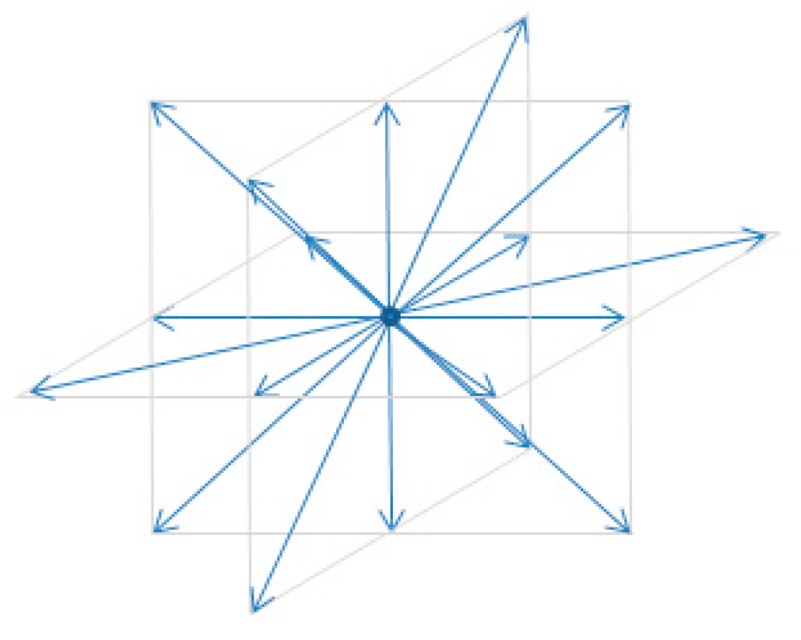
ei is the
ith of the 19 velocity vectors at each node (
Figure 1) which are defined as
where
c =
dx/
dt is the lattice speed. The lattice spacing
dx and time-step
dt are both unity.
The equilibrium distribution
fEq(
ρ,
u) and forcing term
F are then computed from the density and velocity of the node where the components are [
21]
Here wi is the weight coefficient for the corresponding velocity vector, given by w0 = 1/3, w1−7 = 1/18, w8−18 = 1/36 and I is the identity matrix.
The post-collision distribution function
f′(
x,
t) is computed using the MRT operator
where
M is the orthogonal matrix which transforms the distribution function into moment space and
M−1 is its inverse.
S is the diagonal matrix of relaxation rates for each moment. Full details of the MRT model can be found in [
13]. Finally, the post-collisional distribution is streamed to the neighbouring nodes
To illustrate how accuracy is lost when computing the algorithm numerically, we consider an expansion of the summations involved in computing the macroscopic velocity at the node
Each component of the velocity is a summation of differences (subtractions). Physically this is the difference between vectors of opposing direction (
Figure 1). If the node velocity is very small (and hence the distribution is quite symmetric), these differences can become smaller than the ability of the floating point data type to resolve, and the calculation becomes unstable.
Floating point types are stored as two parts: a mantissa (1.2666665) and exponent (−1) in the example
The mantissa in single precision (4-byte float) types is accurate to around 7 decimal places (in base 10), and the exponent ranges from −38 to +38. Therefore a difference can only be resolved to an accuracy of 10
−7 the largest value in the negation. For a node with a small velocity, and distribution close to the zero-velocity (equilibrium) distribution
f0(
ρ0 = 1,
u0 =
0), defined in D3Q19 by
only velocities larger than
O(10
−2) ⋅ 10
−7 = 10
−9 can be resolved at all, and the calculation is verifiably unstable when velocities are less than 10
−7 since only a few decimal places accuracy is maintained.
When computing the flow in complex geometries, often with minimal connectivity, the magnitude of the velocity vectors can become smaller than this. A double precision implementation can handle this easily, but comes with the drawback of requiring considerably more compute time and memory than float precision. The small velocity can, in some cases, be counteracted by choosing a larger body-force. However if this is too large, it can exceed the model stability limits and the calculation will fail. Non-Darcy effects may also begin to appear in faster flow paths if the Reynolds number becomes too high [
22]. In these cases, slow flows are desirable for accurate permeability calculation. Ideally, it should not become an art to choose an appropriate body-force for a given simulation domain; often the connectivity in a simulation is not known beforehand.
The calculation variables can be transformed so that greater accuracy is obtained. Instead of storing the distribution function
f(
x,
t), we define a perturbation
df from the zero-velocity distribution in the following way, as was suggested by Skordos [
5]
so that the distribution function at the node is decomposed into a reference distribution, chosen as the zero-velocity equilibrium distribution
f0(
ρ0,
u0) with
ρ0 = 1 and
u0 =
0, and a perturbation
df. The appropriateness of this transformation rests on the lattice Boltzmann algorithm being memory-bandwidth-limited. This means that it would be preferable to compute the full distribution function locally by adding together
and
dfflt using double precision arithmetic (and where the subscripts
dbl and
flt express the variable’s data type), storing
df as a single-precision (float) data type in the main memory. However, even this is unnecessary if we transform the macroscopic quantities
Although we are still computing differences in the expression for velocity, the zero-velocity expression for the distribution df is 0, so these differences are not bound by the order of magnitude of the calculation values, and are computed to full 7 d.p. accuracy. Note that the expression for the local density is still bound by the order 100.
The difference
fEq −
f which arises in the collision term should be considered as well to maximise the accuracy of the calculation. Writing this in terms of the deviation distribution
df, and using the subscripts
dbl and
flt to indicate the precision (double and single respectively) to which the variables might be stored or calculated, we obtain
The difference could be computed to double precision and converted back to single precision afterwards. This is because the node distribution and equilibrium distribution will be of order 10−1, but the difference often considerably smaller.
Finally though, the need for double precision can be avoided completely if we first compute the equilibrium distribution as a perturbation from the zero equilibrium
dfEq =
fEq(
ρ,
u) −
f0(
ρ0,
u0) such that
The density difference
ρ −
ρ0 will be small relative to the density values of order 10
0. However, this calculation can be made more accurate if we identify the following
We must explicitly compute this density difference from the right hand side summation and not via the densities themselves, otherwise precision is lost. This substitution is particularly important in the low velocity limit and was not mentioned in Skordos’ original paper which only considered how the now comparable magnitudes of each term in (our) Equation (14) increases accuracy under addition, rather than the precision of each individual term [
5]. Using the transformed quantities, the evolution of the LB equation is given as
In the single-relaxation-time (BGK) scheme, the collision part would similarly be written with a relaxation time
τ 3. Results
The two methods of calculating the collision term are compared by computing the velocity distribution
U(
x) between two infinite parallel plates of separation
L (
Figure 2), for which the analytical solution is well known, using a viscosity
μ and body-force component
g in a direction parallel to the plates:
The method in which the complete distribution function is used, Equation (5) is referred to as the distribution method, and the scheme evolving the perturbation from the zero distribution, Equation (16) is referred to as the perturbation method. The deviation from the analytical solution for each method is computed as the relative error
where
u(
x) is the computed velocity component in the body-force direction as a function of position
x between the plates.
For assuredly good convergence, computations are run for 10
6 time-steps. The error is shown in
Figure 3 for the distribution and perturbation methods using respectively float (single-precision) data types and double (precision) data types. The body force used was
g = 10
−6 in dimensionless lattice units (Lu) and the viscosity
For this system, the perturbation methods are consistently 2 to 3 orders of magnitude more accurate than the distribution method of the same data type, though the perturbation method with float precision cannot match the accuracy of the double-precision distribution method in this calculation.
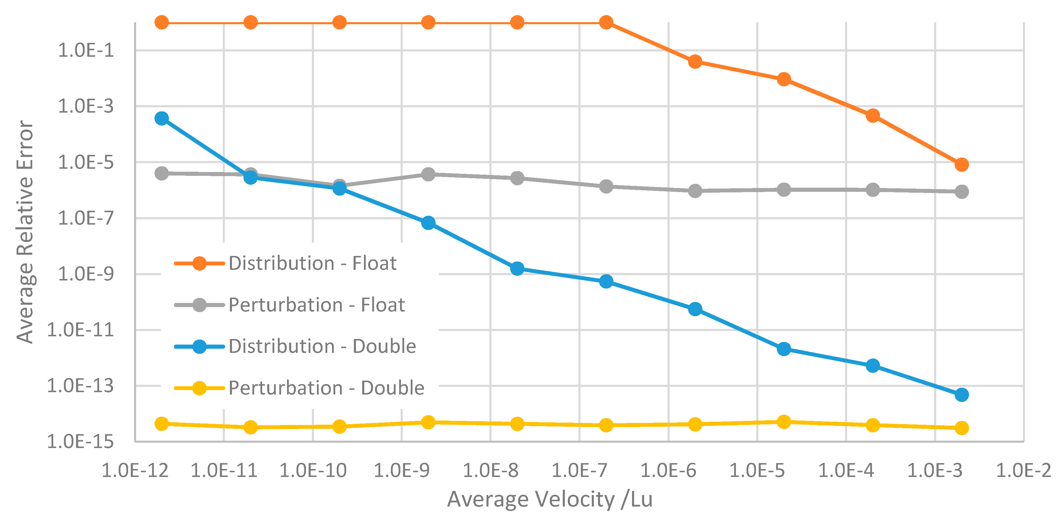
To illustrate how the accuracy of the perturbation scheme is freed from dependence on the magnitude of the velocities, the relative error averaged across the flow profile is plotted in
Figure 4 for different average flow velocities. These were obtained by systematically reducing the body-force. It is clear that as the distribution methods lose accuracy for lower lattice velocities, the perturbation methods maintain a consistent relative error. We also note that the accuracy of the distribution methods converge to those of the perturbation schemes as the magnitude of the velocities approaches that of the zero equilibrium distribution Equation (9). Finally, the accuracy of the perturbation method with float precision can exceed that of the distribution method with double precision at grid velocities below around 10
–11.
To demonstrate the practical advantages of the enhanced accuracy afforded by the perturbation scheme at low velocities, we compute the flow in a 3D pore space image of a Portland carbonate rock sample (
Figure 5 and
Figure 6) obtained from micro-CT imaging [
10]. The sample is 400
3 lattice units in size, but reflected about the
x = 0 plane to give continuous loop boundary conditions so that a body-force may be used [
10]. The structure of the pore-space is highly heterogeneous and of low permeability. The body-force used was again
gx = 10
−6 and the viscosity
.
The average velocity throughout the medium is given over the simulation time for the different schemes in
Figure 7. Most strikingly, the distribution method using floating point precision exhibits a large, systematic deviation from the double precision calculation of almost 50% and as such would give an overestimate of the permeability by the same amount. The perturbation method with float precision on the other hand matches the double-precision distribution calculation closely, yet requires considerably less memory and computing time to perform. Run on a Tesla K20 GPU, the float precision calculations required 27.8 s per 1000 time-steps and the double precision calculation required 48.3 s. In our sparse grid implementation, the array indices of each fluid node’s 18 neighbours are also read in from the memory. Since these are stored as 4-byte integers in both float and double implementations, the speed up of 1.74x is in line with a memory-bandwidth-limited model.


