Article

Clustering versus Incremental Learning Multi-Codebook Fuzzy Neural Network for Multi-Modal Data Classification

by
Muhammad Anwar Ma’sum
*,†,
Hadaiq Rolis Sanabila
,
Petrus Mursanto
and
Wisnu Jatmiko
Faculty of Computer Science, Universitas Indonesia, Kampus Baru UI Depok, Jawa Barat 16424, Indonesia
*
Author to whom correspondence should be addressed.
Current address: R. 1231 Gedung A Fakultas Ilmu Komputer Universitas Idonesia Kampus UI, Depok 16424, Jawa Barat, Indonesia.
Submission received: 28 October 2019 / Revised: 3 January 2020 / Accepted: 4 January 2020 / Published: 13 January 2020

Abstract

:
One of the challenges in machine learning is a classification in multi-modal data. The problem needs a customized method as the data has a feature that spreads in several areas. This study proposed a multi-codebook fuzzy neural network classifiers using clustering and incremental learning approaches to deal with multi-modal data classification. The clustering methods used are K-Means and GMM clustering. Experiment result, on a synthetic dataset, the proposed method achieved the highest performance with 84.76% accuracy. Whereas on the benchmark dataset, the proposed method has the highest performance with 79.94% accuracy. The proposed method has 24.9% and 4.7% improvements in synthetic and benchmark datasets respectively compared to the original version. The proposed classifier has better accuracy compared to a popular neural network with 10% and 4.7% margin in synthetic and benchmark dataset respectively.

1. Introduction

Classification is a machine learning method that is used widely in various areas such as human science, health, e-commerce, and robotics. The method is used to predict the output class label based on the data feature. One of the open problems in classification is classification in multi-modal data [1]. In the real world, the distribution of data is not always unimodal. In some cases, we will face multi-modal data where the feature of the data is distributed in multiple areas. For example, several users in e-commerce have different preference for the same choice (item). Another example is the prediction of an election results. A candidate is voted by residents that aged below 30 (0–30) and in range (40–60). While the other candidate is voted by residents in age (25–45) only. We can say that the first candidate (class) has multi-modal data as its feature spreads in two areas. Gathering the data from such condition will produce a multi-modal data, a data characteristic that has multiple peaks when its distribution is drawn. In other words, we can say that the data has mixed multiple distribution. As the data has multiple peaks it needs custom techniques to analyze the data itself [2,3]. The study of multi-modal data analysis is conducted in the various area e.g., facial expression, sentiment analysis, medical image analysis, video analysis, and surveillance [4,5,6,7,8]. The other researches have been conducted in the special case of multi-modal classification such as large-scale and real-time multi-modal classification [9,10].There are several approaches proposed to solve classification in multi-modal data, such as using a more complex architecture classifier with kernel combination, incremental learning, and ensemble learning [11,12,13].
To deal with multi-modal data, the original (single-codebook) classifier is not able to fit the data properly. The data feature spreads in multiple areas while the methods only approximated by using single preference (codebook). When the feature of the classes is not overlapping, then there is no problem. But if the feature is overlapping, then It will cause misclassification. For example, in the election case as mentioned above. Let class A has a feature in range (0–30) and (40–60) while class B has a feature in range (25–45). The single preference (codebook) classifier will have one reference for each class where class A is in range (0–60) and class B is in range (25–45). We know that (25–45) is in (0–60) which means class A and B is highly overlapping. In this case, the classifier will find difficulty to separate those classes. In multi-codebook approach, the classifier will have two references for class A (0–30) and (40–60). It means in class A and B are less overlap in this case. According to Baltrusaitis et al., the multi-modal can be represented by two representations as shown in Figure 1 [1]. One of the representations is the joint representation notated as x m = f ( x 1 , x 2 , x n ) . The function f is a joint function that is computed by machine learning methods such as neural networks or restricted Boltz-mann machine. The other representation is coordinated representation notated as f ( x 1 ) g ( x 2 ) . The function f and g are the mapping function that maps the unimodal distribution into multi-modal distribution. The coordination between f and g is notated by the symbol (∼). The explanation aout the idea and motivation of using multi-codebook to solve multi-modal data is written in Section 4.
In the previous study, we have been developed a method called Multi Codebook Learning Vector Quantization (MC-LVQ), which is based on clustering technique [14]. The idea is developing a simple neural network architecture by generating multiple reference vector (codebook) of each class. The number of codebooks in each class is independent of other classes. The codebooks are generated by using clustering in the codebook initiation before the training process. We tried three clustering methods: K-Means [15], Gaussian Mixture Model (GMM) [16], and Intelligent K-Means (IK-Means) [17]. IK-Means clustering is a non-parametric version of K-Means that the method does not need the number of clusters as input. Although it’s convenient in the clustering process, for generating codebook in neural network classifiers, it has lower performance than standard (parametric) K-Means.
This study is a continuation of our previous study [14]. First, In this study, we proposed further observation of multi-codebook neural network using clustering. We investigate the number of clusters to the number of peaks in the dataset. In this study, we also investigated the impact of cluster pruning for classifier performance. Second, we proposed a new version of multi-codebook neural network that is developed using incremental learning approaches. Third, we compare the multi-codebook neural network using clustering and incremental learning in the synthetic dan benchmark dataset. In addition, we also compared the proposed method with existing popular neural networks, such as multi-layer perceptron (MLP), Deep Believe Network (DBN), Stack Auto Encoder (SAE), and Extreme Learning Machine (ELM) [18,19,20,21].
This paper is written into six sections. The first section is the introduction of the study. The second section is the related works. The third section is the method which contains explanations of preliminary methods and our proposed method. The fourth section discusses the proposed method in detail. Then, the fifth section is the experiment results also with the analysis. The last (sixth) section is the conclusion of the study.

2. Related Work

Real-world data commonly comes in different characteristics or modalities. For example, same class of images and textual data have different characteristics and statistical properties. Images are represented in pixel intensities. Meanwhile, textual data is represented in sequences of words. Integrating different sources of data is taken in order to obtain a better view on analyzing data. Thus, it is very important to discover the correlation between different modalities. In another case, multi-modality is produced by different atributes (features) for the same category (class). For example, two patients of disease have different profiles. Multi-modal classification is one of the classification tasks that analyzes multi-part models data. The data consist of multiple parts models that may overlap or have deficient coverage.
Many types researches have been done to address the multi-modal data. Fluery et al. [22] proposed an SVM based method to analyze the daily activities data acquired from multiple sensors. The acquired data is extracted using PCA and the corresponding multiple-source data classified using multiclass SVM. Molina et al. using incremental SVM to classify prostatic adenocarcinoma [12]. Zhang et al. study on multi-modal classification of Alzheimer’s disease [11]. al Ortiz et al. using an ensemble deep learning for Alzheimer’s disease classification [13]. Gomez-Chova et al. [23] observing the multi-modal classification in remote sensing areas by employing some advanced methods such as kernel-based method, dictionary learning method, and deep learning. Gallo et al. [24] exploring the multi-modal classification fusion on textual and image data. Ignazio using bag of word feature on text data and deep CNN feature that extracted from the image. Based on the experiment, the proposed method performs better even the dataset contains ambiguity. In the biomedical area, Chambon et al. [25] using deep learning for sleep stage classification.
Learning Vector Quantization (LVQ) [26] is a classification method that has a simple approach and low running time. In the learning stage, each data is represented as a vector. Then, it will compute the distance between the input vector and the reference vector and chooses the closest vector as the winner. The winner vector will be updated in the epoch. Unfortunately, the reference vector does not converge well, and it will degrade the LVQ performance. GLVQ [27] was proposed to tackle the LVQ problem by using a cost function to approximate the reference vector. Many researchers have proposed the extension of LVQ. Setiawan et al. [28] used a fuzzy membership function into the LVQ learning stage (FNGLVQ). FNGLVQ (Fuzzy Neuro Generalized Learning Vector Quantization) solved the overlapping distribution in arrhythmia data. Moreover, Rachmadi et al. [29] proposed the combination of FNLVQ and PSO. PSO is employed for seeking the best cluster in FNLVQ. Unfortunately, PSO will add the complexity of the network and learning time. LVQ based method has been widely used in classification tasks such as in hyperspectral image classification, arrhythmia classification, and handwritten recognition. Recently, multi-modal data is analyzed using a neural network-based method. Parisi et al. [30] using neural network self-organization for analyzing the multi-sensory information in an autonomous robot. Lu et al. [31] using Deep neural network for diagnosing Alzheimer’s. In this work, we will compare our proposed method with the neural network-based method such as Multi-Layer Perceptron (MLP), Stacked Auto Encoder (SAE), Deep Belief Network (DBN), and Extreme Learning Machine (ELM).
As stated in the previous section, our proposed method is based on FNGLVQ. In the traditional FNGLVQ, we build a single codebook from the input data. The codebook of the data will be build based on the min, mean, and max of the data. This approach is fast and effective for a single peak (uni-modal) dataset. However, the traditional approach has performance issues in the multi-modal dataset as It can’t cover all the data distribution accordingly.
In this study, we use a multi-codebook approach in order to fit a multi-modal data. In the first approach, we use clustering to generate a multi-codebook by clustering the input data. While in the second apporach, we use incremental learning to generate a new codebook gradually during training process. The new codebook is generated when the classifier find the condition to generate it. The detail of the proposed method is explained in Section 4.

3. LVQ-Based Neural Network

3.1. Learning Vector Quantization (LVQ)

Proposed by Kohonen [32] in 1986, Learning Vector Quantization (LVQ) is one of the supervised learning based on a distance measure. The LVQ’s main idea is to pull the winner codebook closer to the input vector if they are in a similar class. Meanwhile, the input vector and winner codebook is in a different class, moved the winner codebook away from the input vector. The architecture of LVQ consists of two layers: the input layer and the output layer. The illustration of the LVQ architecture depicted in Figure 2.
Given input vector (x), class label (Y), and reference vector ( w i j ) of class j for feature i. The input vector is an instance of training data. In the beginning, the reference vector ( w i j ) for each class is initiated by random sampling from the training sample. Then the reference vector ( w i j ) is updated by using Equations (1) and (2). First, the method computes the distance between input and reference vector of all class (all variation of j) by using Equation (1). Then the method finds the winner class. Winner class is denoted as w and the reference vector (codebook) of winner class is denoted as w w . The value of w is one of j possible values. For example if we have three classes j = 1 , 2 , 3 then w could be 1, or 2 or 3. Winner class is a class that its distance is closest (minimal) to the input vector. Then the reference vector of winner class ( w w ) is updated by using Equation (2). The process is conducted for all input vectors (training instances) and It is conducted for a number of iteration (epoch).
d ( j ) = i = 1 N ( x i w i j ) 2
w w ( t + 1 ) = w w ( t ) + α ( x w w ( t ) ) , i f Y ( w w ) = Y ( x ) w w ( t ) α ( x w w ( t ) ) , i f Y ( w w ) Y ( x )

3.2. LVQ 2.1

LVQ 2.1 is the improvement of LVQ 1 by considering the runner up reference vector and winner reference vector. This method uses a window constant ( ω ) for limiting the update phases. It has the consequence that will juxtapose the winner reference vector and alienate the runner up reference vector ( w r ) from the training sample. The update phases are conducted if the entire condition is sufficed.
Y ( w r ) Y ( w p ) , a n d d ( w p ) d ( w r ) > ( 1 ω )
where d ( w r ) is the distance between runner up vector and training sample, whereas d ( w w ) is the distance between the winner vector and training sample. Then w r and w w have to be updated according to the formulas (4) and (5).
w w ( t + 1 ) w w ( t ) α ( x w w ( t ) )
w r ( t + 1 ) w r ( t ) + α ( x w r ( t ) )

3.3. Generalized Learning Vector Quantization (GLVQ)

Generalized Learning Vector Quantization (GLVQ) is one of the LVQ improvement that widely used. This method was proposed by Sato and Yamada [27] in 1998. During the learning process, GLVQ minimizing the misclassification error and cost function. Supposed w a is the reference vector of the input vector (class of w a = class of w x ) and w b is the closest reference vector from dissimilar class (class of w b ≠ class of w x ), the misclassification error is specified as formula (6) below.
e ( x ) = ( d a d b ) d a + d b
where d a and d b is the distance between w a and w b to input vector x.
To enhance the classifier performance, the misclassification error should be decreased during the learning process. So thus, the misclassification error should be minimized according to cost function in formula (7).
M = i = 1 N f ( e ( x ) )
Sato et al. use sigmoid function as monotonically increasing function (f) [27]. Moreover, the steepest descent method is employed to minimize M. Hence, the updating rules for w a and w b are defined in formula (8).
w k ( t + 1 ) w k ( t ) α δ M δ w k ( t ) , k = a , b
If Euclidean distance is employed, thus formula (8) can be composed as formulas (9) and (10).
δ M δ w a = δ M δ e δ e δ d a δ d a δ w a = δ f δ e 4 d b ( d a + d b ) 2 ( x w a )
δ M δ w b = δ M δ e δ e δ d b δ d b δ w b = δ f δ e 4 d b ( d a + d b ) 2 ( x w b )
As a result, the updated rules for w a is described in formulas (9) and (10). Meanwhile, the updated rules for w b is described in formulas (11)–(14).
w a ( t + 1 ) w a ( t ) + α δ f δ e 4 d b ( d a + d b ) 2 ( x w a ( t ) )
w a ( t + 1 ) w a ( t ) + α f ( φ , t ) ( f ( φ , t ) ) 2 4 d b ( d a + d b ) 2 ( x w a ( t ) )
w b ( t + 1 ) w b ( t ) + α δ f δ e 4 d a ( d a + d b ) 2 ( x w b ( t ) )
w b ( t + 1 ) w b ( t ) + α f ( φ , t ) ( f ( φ , t ) ) 2 4 d a ( d a + d b ) 2 ( x w b ( t ) )

3.4. Fuzzy-Neuro Generalized Learning Vector Quantization (FNGLVQ)

Made Agus et al. proposed the improvement of GLVQ for tackling high intersection data by using fuzzy logic [28]. The proposed method is Fuzzy-Neuro Generalized Learning Vector Quantization (FNGLVQ). The illustration of FNGLVQ architecture can be seen in Figure 3.
Supposed λ is the similarity value between the input vector and reference vector from a similar class and λ b is the similarity value between the input vector and the closest reference vector from dissimilar class, then the distance can be defined into d = 1 λ . Furthermore, by substituting the distance ( d = 1 λ ) into formula (6), the misclassification error can be defined to formula (15).
e ( x ) = μ b μ b 2 ( μ b + μ a )
The misclassification error should be minimized to improve the classifier accuracy. Thus, the learning criteria are formulated by deriving cost function toward w k .
δ M δ w k = δ M δ e δ e δ μ δ μ δ w k , k = a , b
In this paper we use triangular membership function w ( w m i n , w a v g , w m a x ) . The similarity value is formulated as below.
λ = 0 , x x w m i n w a v g w m i n , w m i n x w a v g w m a x x w m a x w a v g , w a v g x w m a x 0 , x
Supposed w a is the reference vector of the input vector (class of w a = class of w x ) and w b is the closest reference vector from dissimilar class ( c l a s s o f w b c l a s s o f w x ). The derivation of cost function lead into 3 cases, i.e.,
  • Case 1: w a v g < x w a v g
    w a ( t + 1 ) w a ( t ) α δ f δ λ 2 . ( 1 μ b ) ( 2 μ a μ b ) 2 ( x w m i n ( w a v g w m i n ) 2 )
    w b ( t + 1 ) w b ( t ) + α δ f δ λ 2 . ( 1 μ a ) ( 2 μ a μ b ) 2 ( x w m i n ( w a v g w m i n ) 2 )
  • Case 2: w a v g < x < w a v g
    w a ( t + 1 ) w a ( t ) + α δ f δ φ 2 . ( 1 μ b ) ( 2 μ a μ b ) 2 ( w m a x x ( w m a x w a v g ) 2 )
    w b ( t + 1 ) w b ( t ) α δ f δ φ 2 . ( 1 μ a ) ( 2 μ a μ b ) 2 ( w m a x x ( w m a x w a v g ) 2 )
  • Case 3: x w m i n   a n d   x w m a x
    w i ( t + 1 ) w i ( t ) , i = a , b
Then w m i n and w m a x is updated based on formulas (23) and (24).
w m i n w a v g ( t + 1 ) ( w a v g ( t ) w m i n ( t ) )
w m a x w a v g ( t + 1 ) ( w a v g ( t ) w m i n ( t ) )
The learning rate ( 0 α 1 ) value is decreasing along with the iteration (t). The learning rate update is following the formula (25).
α ( t + 1 ) α 0 x ( 1 t t m a x )
In addition, the membership function w ( w m i n , w a v g , w m a x ) should be adjust according 3 cases below.
  • Case 1: ( ( μ a > 0 or μ b > 0 ) and e < 0 ) , where β is constant ( 0 β 1 )
    w m i n w a v g ( w a v g w m i n ) ( 1 + ( β . α ) )
    w m a x w a v g + ( w m a x w a v g ) ( 1 + ( β . α ) )
  • Case 2: e 0 , where β is constant ( 0 β 1 )
    w m i n w a v g ( w a v g w m i n ) ( 1 ( β . α ) )
    w m a x w a v g + ( w m a x w a v g ) ( 1 ( β . α ) )
  • Case 3: ( μ a = 0 and μ b = 0 ) . where γ is constant ( 0 γ 1 )
    w m i n w a v g ( w a v g w m i n ) ( 1 ( γ . α ) )
    w m a x w a v g + ( w m a x w a v g ) ( 1 ( γ . α ) )

4. Proposed Method: Multi-Codebook Fuzzy-Neuro Generalized Learning Vector Quantization (MC-FNGLVQ)

In this paper, we proposed Multi Codebook Fuzzy Neuro Generalize Vector Quantization (MC-FNGLVQ). There are two approaches to generate multi-codebook FNGLVQ. The first approach is using clustering to initiate codebook, and the second approach is using incremental learning during the training process. The details of the methods are explained in the subsections.

4.1. Problem, Motivation, and Idea
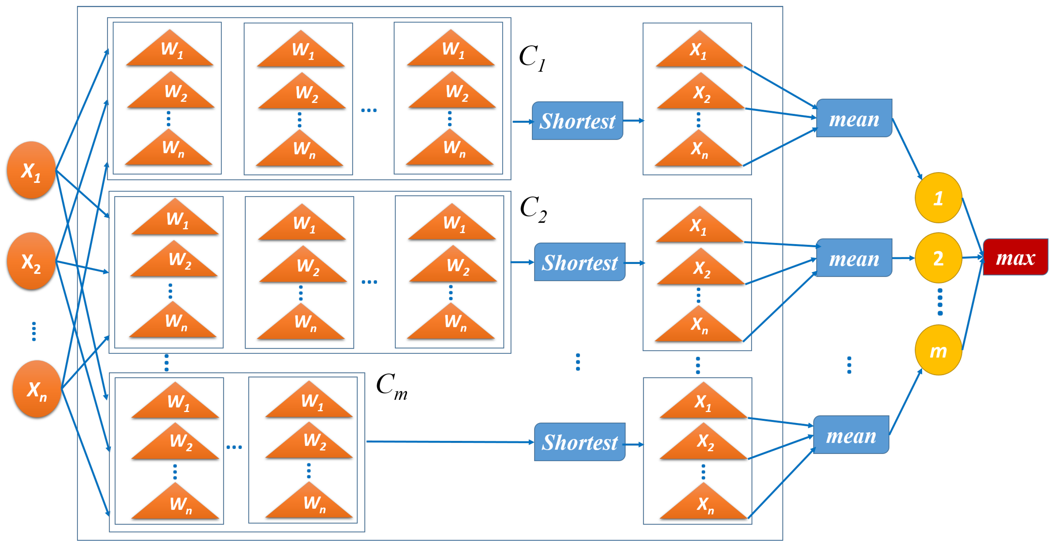
As mentioned in the introduction section, multi-modal data is data that its feature spreads in multiple areas. Figure 4 ilustrates a simple dataset with multi-modal characteristic. Let’s focus on the feature-X (feature on x-axis). The figure shows the feature of class A (blue) spreads into two areas while the feature of class B (red) spreads only in one area. Feature of class B is in an area between areas of the featurea of class A. If we draw the distribution of each group of data, then we have two distribution for class A and one distribution of class B. The reference (codebook) generated by neural network for the feature of each class is ilustrated by triangle shape. The reference will accommodate the area of the feature. A single-codebook approach is shown in the top diagram where the reference of class A and class B are highly overlapping. While multi-codebook approach is shown in the bottom diagram where It has less overlapping references. Therefore, in this study, we proposed a multi-codebook approach for neural network to deal with multi-modal data.
In this study, we proposed two approaches for generating multi-codebook. The first approach is by using the clustering method. Before the training process, the data of each class is clustered. It will produce several groups (clusters) of data. Each cluster is used to generate a codebook (reference vector) for the associated class. During training process, the method will update the closest reference vector to the input among all reference vectors produced before. The other method is using incremental learning. The idea is gradually generating new codebook during training process when necessary. Before training, the method generates single-codebook as in the original version. During the training process, the method will check if It is necessary to generate a new codebook (reference vector). If yes, then the method will generate a new codebook for class associated with input data (instance). The detail of the methods is explained in the following sub-sections.

4.2. Architecture

The architecture of multi-codebook FNGLVQ is shown in Figure 5. From layer perspective, the architecture of multi-codebook FNGLVQ is similar to original FNGLVQ, which uses a single hidden layer. The input layer and the output layer have no different from the original FNGLVQ. The basic idea of multi-codebook FNGLVQ is using multiple reference vector (multi-codebook) in the hidden layer to approximate the multi-modal dataset. In the original FNGLVQ, each class has only one reference vector (codebook), whereas, in multi-codebook FNGLVQ, each class has several reference vectors.
In this study, the vectors are generated by using clustering and incremental learning. Therefore, there are two versions of the multi-codebook FNGLVQ discussed in this paper. The first version is using a clustering approach to generate a reference vector, and the second version is using an incremental learning approach. The details of these versions are explained in the following sections.

4.3. Multi-Codebook Fuzzy-Neuro Generalized Learning Vector Quantization (MC-FNGLVQ) Using Clustering Approach

One of the versions of the method is multi-codebook FNGLVQ using a clustering approach. In this method, the reference vectors of each class are generated using the clustering method. The idea of clustering is to divide the data into several groups. Then, each group will be approximated using a reference vector. Therefore, before the training process, the clustering process is performed. The clusters (a group of data) are used to generate reference vector candidates. The candidates will be updated during the training process to approximate the group of data. By using this approach, the classifier is expected to fit data with multi-modality. The clustering used in multi-codebook FNGLVQ is K-Means and Gaussian Mixture Model (GMM) clustering.
There are several processes in multi-codebook FNGLVQ based on a clustering approach. First, the dataset is divided by class label. Then, the data of each class is clustered into the C cluster. Afterward, the cluster with a small member is pruned. The pruning process is optional. The clusters (group data) of a particular class are used to generate reference vector candidates if the class by performing fuzzification. Fuzzification is a process calculating min, mean, and max of the data. If there are many attributes (features) in the data, then the calculation is performed to each attribute. The training process of the proposed method is conducted using steps in Algorithm 1.
In the testing process, the clustering algorithm is not used. The testing method is the same as the original FNGLVQ, which is found most similar (closets) reference vector. The label of the winner vector is the predicted class label.
Algorithm 1 Multi Codebook Fuzzy Neuro Generalized Vector Quantization Using Clustering.
1:
procedureMC-FNGLVQ-CLustering
2:
    denote x 1 , x 2 , x n as instances
3:
    denote f 1 , f 2 , f m as data features
4:
    denote c 1 , c 2 , c y as class labels
5:
    for i = c 1 : c y do
6:
        C as number of cluster
7:
        denote f c = f 1 , f 2 , f m of class i
8:
        Do Clustering to f c , #cluster=C
9:
        for j = 1 :C do
10:
           denote C j as member of cluster-j
11:
           find m i n , m e a n , m a x of C j
12:
           generate codebook for class j in FNGLVQ method
13:
        end for
14:
    end for
15:
    for x = x 1 : x n do
16:
        train x in FNGLVQ method using Equations (17)–(31)
17:
    end for
18:
    

4.4. Multi-Codebook FNGLVQ Using Incremental Learning Approach

The second version of the method is Multi-Codebook FNGLVQ using an incremental learning approach. In this version, the reference vector This section discusses multi-codebook FNGLVQ using an incremental learning method. The difference from the previous version is that the reference vector candidates are generated before the training process. In this method, the reference vectors are generated during the training process.
The codebook (reference vector) of each class is generated as in the original FNGLVQ. The initiation can be performed by using fuzzification of all data in each class, or fuzzification of selected data. Selected data is chosen by random selection. After initiation, each class has only one reference vector. During the training process, the method will decide if it is necessary to generate a new codebook.
In training iteration, the method is given input vector x as in original FNGLVQ. Then, the method measures the membership value of the input to existing reference vectors of its class. This measurement is performed by using Equation (17). If the input vector is distant to the reference vector, then the method will generate a new reference vector. The threshold of membership value to decide the new codebook generation is set prior to the training process. If a new reference vector is generated, then input value (x) is set as the mean of the new reference vector. Min and max values of the vector are set based on Min-Mean distance and Mean-Max distance of the existing reference vectors. The training process in multi-codebook FNGLVQ using incremental learning is shown in Algorithm 2.
For the testing process in muti-codebook FNGLVQ using incremental learning, the process is the same as the testing process in original FNGLVQ and multi-codebook FNGLVQ using incremental learning. The process is finding the winner (closets) reference vector, and state the label of the winner vector as the predicted class label.
Algorithm 2 Multi Codebook Fuzzy Neuro Generalized Vector Quantization Using Incremental Learning.
1:
procedureMC-FNGLVQ-Clustering
2:
    denote x 1 , x 2 , x n as instances
3:
    denote t as threshold
4:
    denote w 1 , w 2 , w p as reference vector of class 1 , 2 , p
5:
    initiate w 1 , w 2 , w p
6:
    for x = x 1 : x n do
7:
        y as class label of x
8:
        compute λ of x using Equation (17)
9:
        if λ > t then
10:
           train x using Equations (18)–(31)
11:
        else
12:
           State w y n e w as new codebook for class y
13:
            w y n e w m e a n = x
14:
            w y n e w m i n = x− average( w y m e a n w y m i n )
15:
            w y n e w m a x = x + average( w y m a x w y m e a n )
16:
     end for
17:
  

5. Experiment Result and Analysis

5.1. Dataset

In this paper, we used a synthetic dataset and benchmark dataset to measure the performance of the proposed method. There are nine synthetic datasets used in this research. The dataset has two peaks, three peaks, and five peaks, each of which has two classes, three classes, and five classes. While the benchmark datasets are datasets used were taken from the UCI database, and several taken from previous research. The details of the datasets are given in Table 1.

5.2. Experiment Setup

The proposed method is implemented in Matlab programming. The proposed method is evaluated by using the following parameters: alpha = 0.05, gamma = 0.00005, beta = 0.00005, delta = 0.1 and epoch = 100. Our preliminary try and error is conducted to find the best combination of alpha, beta, delta, and gamma for FNGLVQ. The experiment is conducted by using 2Peak-2Class synthetic dataset. Table 2 shows that for epoch = 100, the chosen value of alpha, beta, and gamma achieved good accuracy among the tested combinations of parameters. Therefore the values are used in the following experiments. In following the experiments, we concerned more about cluster parameters and threshold for incremental learning parameters. The number of clusters is tested as described in scenario 1. As a comparison, the existing method DBN, SAE, and ELM are also implemented in Matlab by using deep learning toolkit. DBN and SAE are tested by using epoch = 100 and hidden layer = 50, 75, 100. The result will be taken from the best layer. We stop on 100 layers because increasing layers from 25 to 100 does not improve performance significantly. Rather, in some cases, the performance is decreasing when the number of layers is increasing. ELM is tested by using epoch = 100. The MLP is also used as comparison. The MLP is implemented in Weka software by using the default setting as follow alpha = 0.3, momentum = 0.2 and epoch = 500. The experiment is conducted by using 5-folds cross-validation.

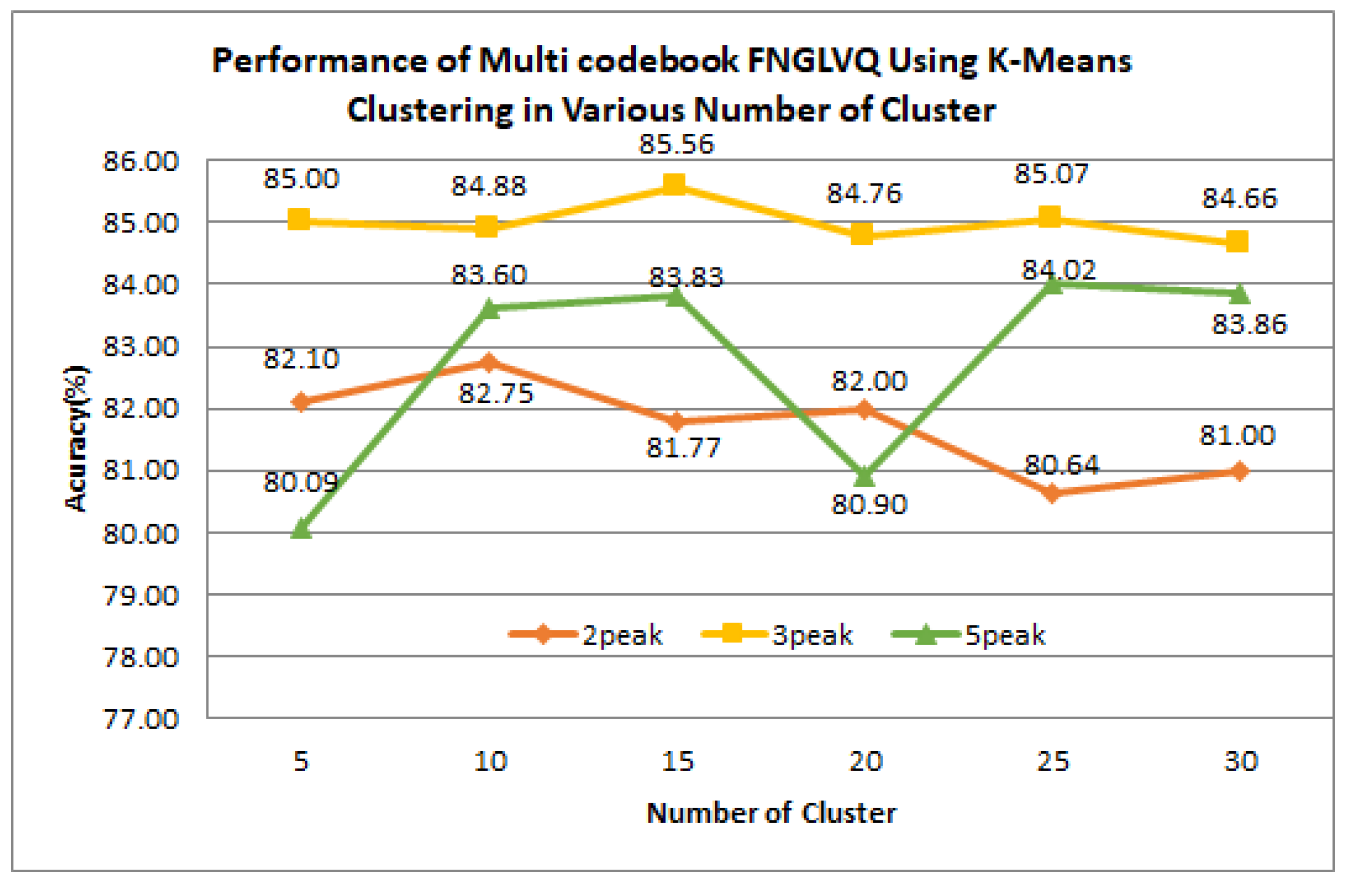
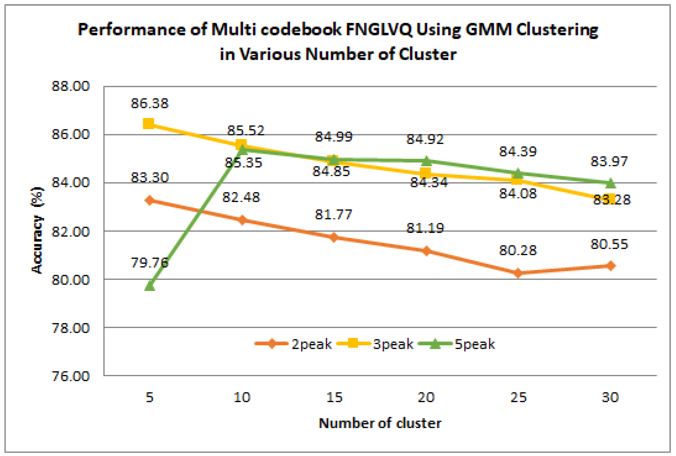
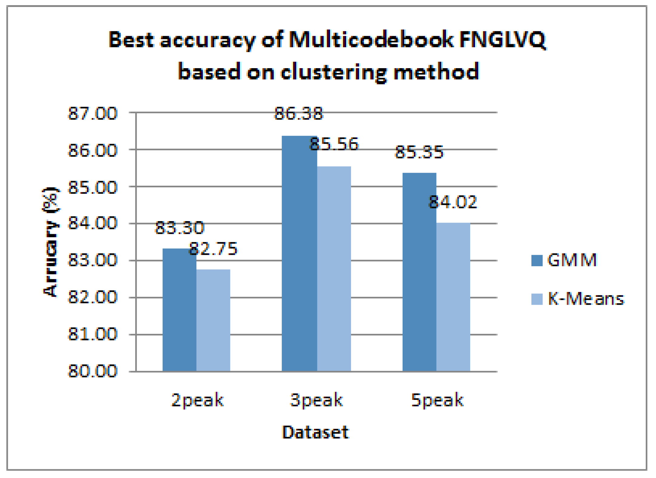
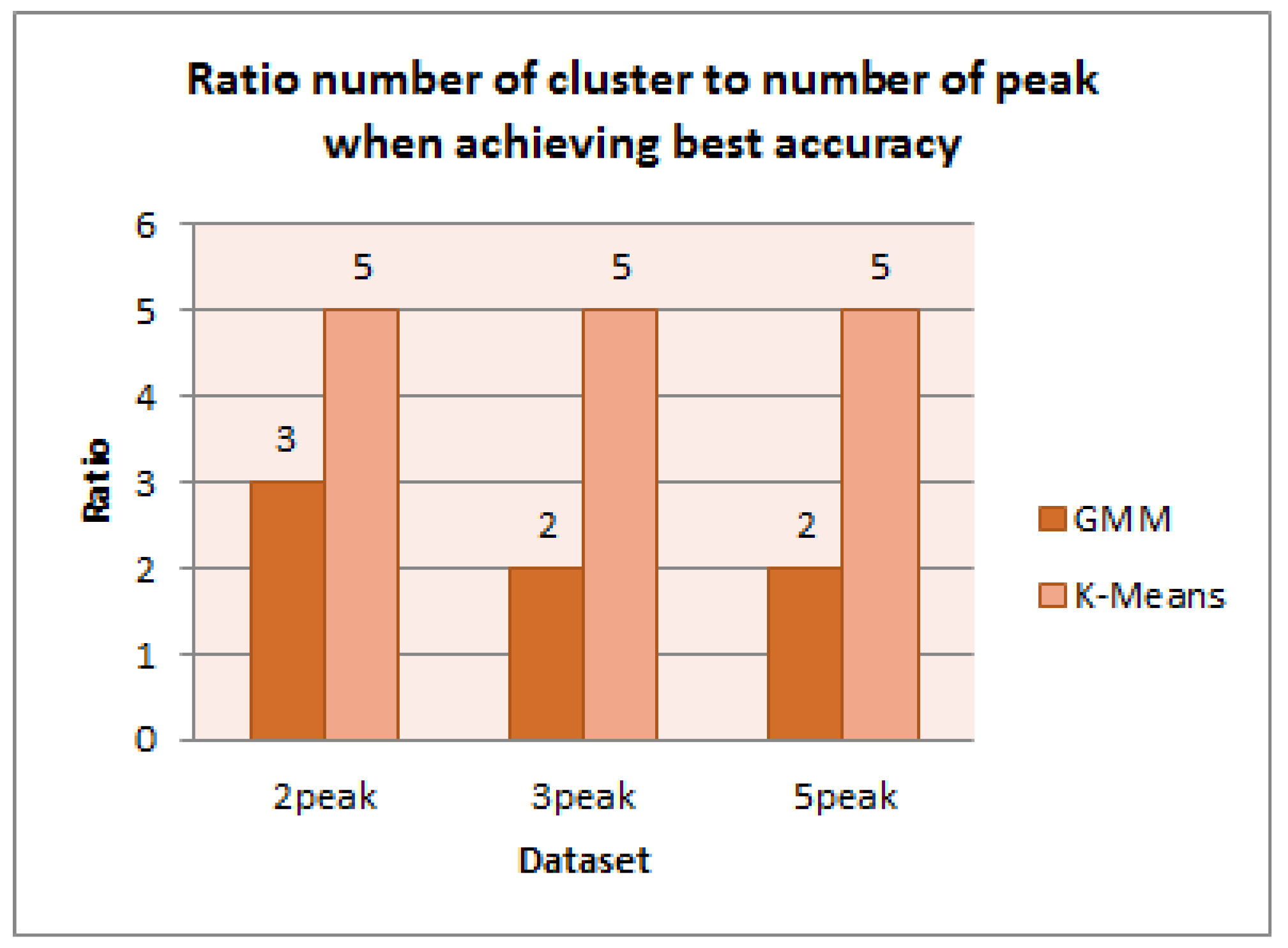
5.3. Result of Scenario 1: The Impact of Cluster Number

In the first scenario, we measure the performance of the proposed methods with a different number of cluster in the dataset with multi-peak. In this scenario, the number of clusters used is from 5 to 30. The experiment result of the multi-codebook classifier using K-Means clustering is shown in Figure 6. Figure 6 shows that for multi-codebook using K-Means clustering in the 2-peak dataset, 10 cluster has the highest accuracy with 82.75%. In the 3-peak dataset, 15 cluster has the highest accuracy with 85.56% accuracy. In the 5 peak dataset, the highest performance is achieved by 25 clusters with 84.02% accuracy.
The experiment result of multi-codebook classifier using GMM clustering is shown in Figure 7. Figure 7 shows that for multi-codebook using GMM clustering in the 2-peak dataset, the highest accuracy is achieved by 5 clusters with 83.30% accuracy. Similar to the occurrence in the 2-peak dataset, in the case of the 3-peak dataset, the highest performance is achieved by 5 clusters with 86.38%. In the 5-peak dataset, the highest accuracy is achieved by 10 clusters with 85.35% accuracy.

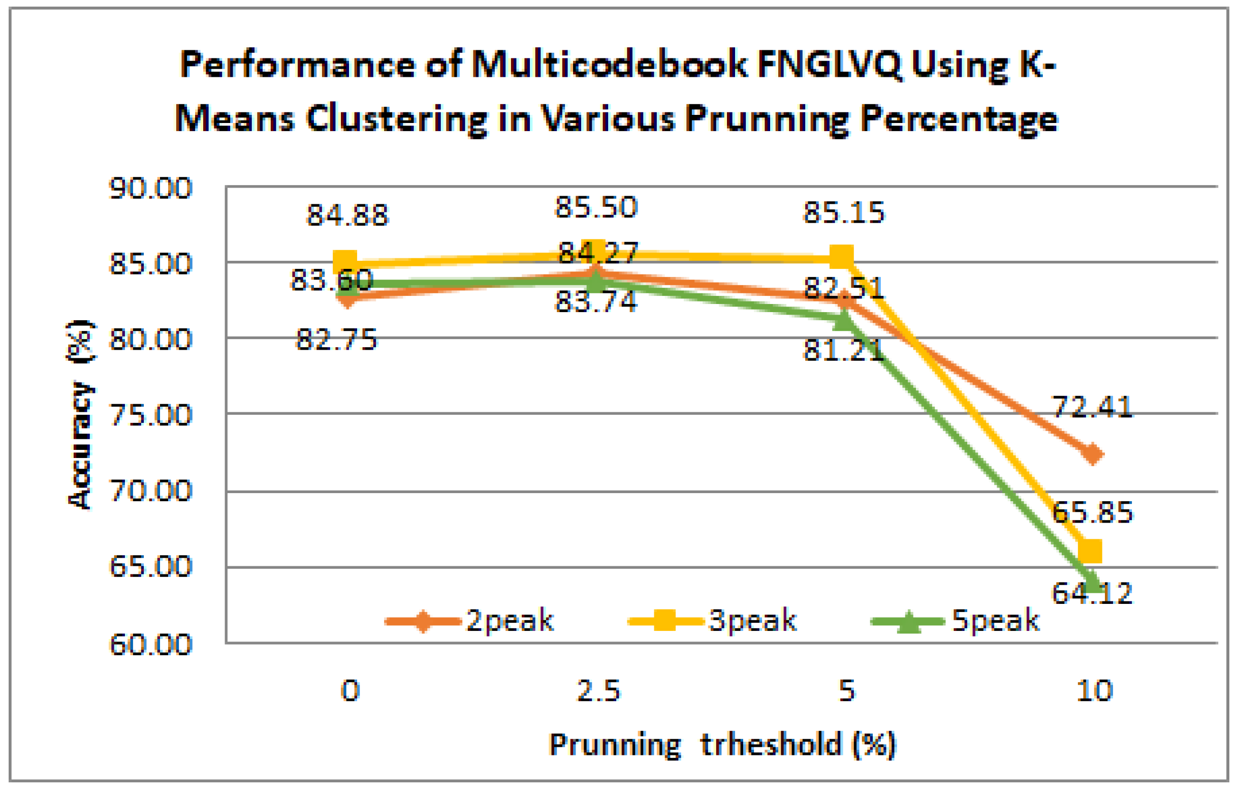
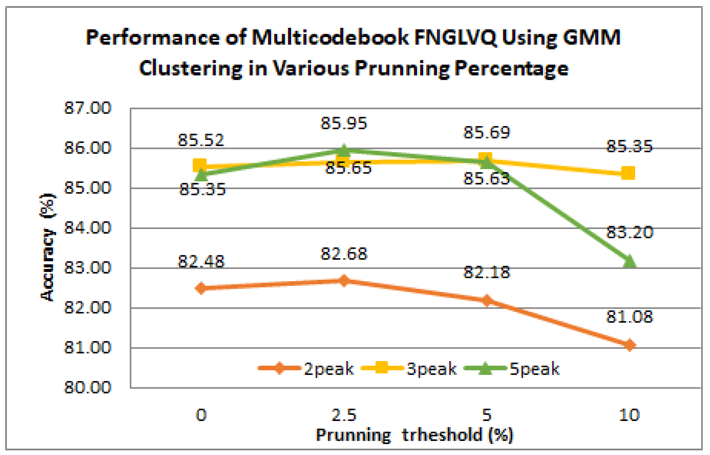
5.4. Result of Scenario 2: The Impact of Prunning

This scenario is used to observe the impact of pruning on the performance of the proposed algorithm. Before generating a codebook, the clusters are evaluated. If the cluster member is less than the minimum threshold, then the cluster is removed, and there is no codebook generated from the removed cluster. The idea if the pruned scenario is to remove the abnormal (outlier) cluster. In this scenario, there are several threshold values used for pruning: 0% (no pruning), 2.5%, 5%, and 10%. The percentage is based on the number of class instances before clustered. The number of clusters used in this scenario is 5 clusters. The result of this scenario is shown in Figure 8 and Figure 9. Figure 8 shows that in multi-codebook FNGLVQ using K-Means clustering. The 2.5% threshold has better accuracy than 0% (no pruning) threshold with approximately 0.7% margin 2-peak, 3-peak, and 5-peak dataset. However, the 5% and 10% threshold have lower accuracy than 0% (no pruning) threshold. Figure 9 shows that in multi-codebookVQ using GMM clustering. The 2.5% threshold has better accuracy than 0% (no pruning) threshold with approximately 0.1–0.6% margin. The 5% threshold also has slightly better accuracy for 3-peak and 5-peak dataset. However, it has lower accuracy than no pruning version in the 2-peak dataset. Similar to the case in multi-codebook using K-Means clustering, the 10% threshold has lower accuracy than no pruning version.
Figure 10 and Figure 11 summarize the best performance of multi-codebook using K-Means and GMM clustering in synthetic dataset. In 2peak, 3peak, and 5peak dataset multi-codebook FNGLVQ using GMM clustering has better accuracy than multi-codebook FNGLVQ using K-Means clustering. The multi-codebook using GMM clustering achieves 83.30%, 86.38%, and 85.35% for 2peak, 3peak, and 5peak, respectively. Whereas, the multi-codebook using K-Means clustering achieves 82.75%, 85.56%, and 84.02% for those three datasets. Figure 11 shows the ratio of the number of clusters to the number of peaks when achieving their best accuracy, as shown in Figure 10. Figure 11 shows that the ratio of the number of clusters to the number of peaks for multi-codebook using GMM clustering is 3 for 2peak dataset, and 2 for 3peak, and 5peak dataset. Whereas for multi-codebook using K-Means clustering, the ratio is 5 for those three datasets. This analysis suggests that dealing with a multi-modal dataset, the number of the cluster for multi-codebook using GMM clustering is two times or three times the number of peak (modal), and the number of clusters for multi-codebook using K-Means clustering is five times the number of the peak (modal).

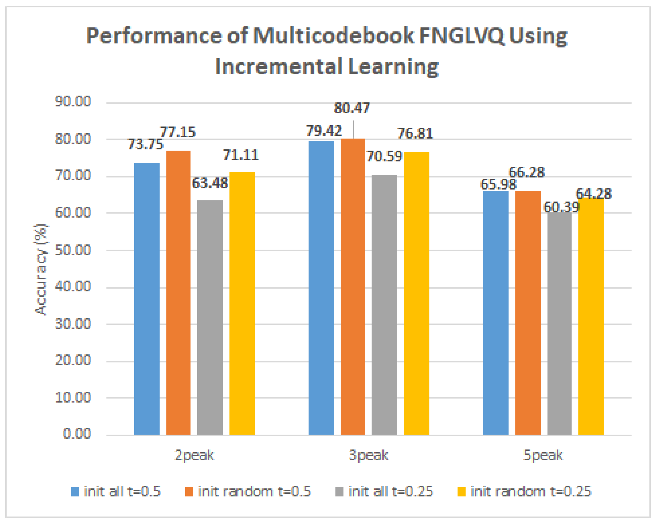
5.5. Result of Scenario 3: Result of Incremental Learning in Synthetic Dataset

This scenario is used to measure the performance of multi-codebook FNGLVQ using incremental learning in the synthetic dataset. In this multi-codebook version, initially, the classifier has one codebook. Then during the training process, when the classifier decides to need to generate a new codebook, then the new codebook is generated. The decision to generate a new codebook is based on the membership value that is shown in Equation (17). If the membership value from respecting class is lower than the threshold, then a new codebook is generated. In this scenario, the threshold used is 0.25 and 0.5. Besides, there are two approaches to codebook initiation: using randomized and using all data. Using all data means that the method read all data to generate its initial codebook for each class, whereas a randomized approach reads randomized sampling data to generate an initial codebook for each class. Figure 12 shows the performance of multi-codebook FNGLVQ using incremental learning in synthetic datasets. Figure 12 shows that the best performance in the 2peak, 3peak, and 5peak synthetic dataset is achieved by the multi-codebook FNGLVQ using incremental learning with 0.5 thresholds and all data initiation. Figure 12 also shows that in the synthetic dataset, for the same initiation method, 0.5 threshold value has better performance than the 0.25 threshold value. Furthermore, Figure 12 shows that in the synthetic dataset, for the same threshold value, random initiation has better performance than all data initiation.

5.6. Comparison of Proposed Method to Existing Methods in Synthetic Data

In this sub-section, the proposed methods are compared to existing neural network classifiers such as MLP, SAE, DBN, ELM, and previous LVQ based classifier. Table 3 shows the comparison of proposed methods to the existing methods. Overall, the multi-codebook FNGLVQ using GMM clustering has the best performance in the synthetic dataset, followed by multi-codebook FNGLVQ using K-Means clustering, MLP, multi-codebook FNGLVQ using incremental learning, DBN, SAE, GLVQ, LVQ2-1, FNGLVQ, and ELM. There are several insights shown in this comparison. First, It is normal that the multi-codebook FNGLVQ using GMM has better performance than the multi-codebook using K-Means clustering because the synthetic dataset used in this experiment has Gaussian distribution. Second, the original FNGLVQ has lower performance than GLVQ and LVQ-21. It shows that to deal with multi-modal data, using fuzzy membership function in the classifier is not always improve its performance. Third, in the synthetic dataset, the MLP has the best accuracy among existing classifiers, and ELM has surprisingly low accuracy compared to others. Fourth, the proposed method achieved 24.9%, 24%, and 13% improvements for multi-codebook FNGLVQ using GMM, K-Means, and incremental learning respectively compared to original FNGLVQ. Compared to MLP that has the best performance among existing methods in the synthetic dataset, the proposed methods have 10% and 9% for multi-codebook FNGLVQ using GMM and K-Means respectively. Whereas, multi-codebook FNGLVQ using incremental learning has slightly lower accuracy than MLP with 0.24% margin.

5.7. Result in Benchmark Dataset

Beside tested in the synthetic multi-modal dataset, the classifiers are also tested in a benchmark dataset that has multi-modal distribution in its features the benchmark dataset are pinwheel and dataset were taken from UCI database as shown in Table 4. In the benchmark dataset, the multi-codebook FNGLVQ using K-Means has better accuracy followed by multi-codebook FNGLVQ using incremental learning, multi-codebook FNGLVQ using GMM, MLP, FNGLVQ, LVQ2-1, ELM, GLVQ, DBN, and SAE. In the benchmark dataset, the proposed methods have 4.7%, 2.8% and 2.4% improvement for multi-codebook using K-Means, incremental learning, and GMM, respectively. In the benchmark dataset, MLP once again achieves the best accuracy among existing methods with 75.82% average accuracy. In this dataset, ELM has better accuracy compared to other existing methods except for MLP with 73.96% average accuracy even tough It has the lowest performance in synthetic dataset. Compared to MLP that has the best accuracy among existing methods, the proposed methods have 4.1%, 2.1% and 1.7% for multi-codebook using K-Means, incremental learning, and GMM, respectively.

5.8. Scoring

In this study, scoring is used to evaluate all classifiers, both in synthetic and benchmark datasets. All ten classifiers were evaluated in each dataset instance. In each dataset instance, the highest accuracy gets 10 points. The second place gets 9 points, third place gets 8 points, and so on, until the lowest classifier gets 1 point. The classifiers that have the same accuracy in a dataset instance get the same points. The scoring table is shown in Table 5. Overall, the highest score is achieved by multi-codebook FNGLVQ using K-Means, followed by multi-codebook FNGLVQ using GMM, multi-codebook FNGLVQ using incremental learning, MLP, DBN, FNGLVQ, LVQ2-1, SAE, and ELM. Multi-codebook FNGLVQ using GMM has a slight lower score compare to multi-codebook FNGLVQ using K-Means with a 0.44 points margin. One performs better in the synthetic dataset while the other performs better in the benchmark dataset.

5.9. Discussion

The proposed method is tested both in the synthetic and benchmark datasets. The synthetic dataset the dataset that all feature of the data has multi-modal distribution. The amount of the modals is two, three and five. Furthermore, the overlapping between classes is high. It is shown in the Appendix A that the distribution of each class highly overlaps with other classes. In the synthetic dataset case, the experiment result shows that the proposed methods improve significantly compared to the original version. Both multi-codebook based on clustering and incremental learning have higher performance compared to the original version on each dataset instances. On synthetic dataset, the proposed method achieved 84.76%, 83.89% and 73.75% for multi-codebook by using GMM clustering, K-Means clustering, and incremental learning respectively, while the original version achieved 59.78%. The multi-codebook by using the GMM clustering version achieved better in this case because the synthetic dataset is generated by using Gaussian distribution. The performance of the proposed methods is indeed still below 90%. For some applications such as medical analysis, It may be not acceptable. However, this study concerns to show that the proposed method improves the original method significantly with improvement up to 24%. Furthermore, the popular classifiers’ achievements on this dataset are also below the proposed method. It shows that the dataset is difficult to classify. However, the good news is the proposed method has room for improvements.
The proposed methods are also tested in the benchmark dataset. The aim of the experiment is to test the method in real dataset. The ionosphere, glass, fertility, spectf, and pinwheel have a sign of multi-modal on their features (but not all features). It shows in appendix figures. While pima and EEG have uni-modal characteristic but the features highly overlap. The experiment result shows that overall the proposed methods achieved better performance than the original version. The best performance is achieved by a multi-codebook by using K-Means clustering with 4.7% improvement compared to the original version. In teh case of pima and eeg dataset, the performance of the proposed methods achieved only small improvement compared to the original. It means that the proposed methods are not recommended for a uni-modal dataset. Instead, the authors recommend the original FNGLVQ for uni-modal classification.

6. Conclusions

In this paper, multi-codebook fuzzy neural network classifiers using clustering and incremental learning approach have been proposed. There are two variations of the classifiers have been developed. The tree variation is multi-codebook FNGLVQ using K-Means clustering, multi-codebook FNGLVQ using GMM clustering, and multi-codebook FNGLVQ using incremental learning. Experiment result, on synthetic dataset multi codebook FNGLVQ using GMM clustering, has the highest performance with 84.76% mean accuracy. Whereas on benchmark dataset multi-codebook FNGLVQ using K-Means clustering has the highest achievement with 79.94% mean accuracy. The multi-codebook FNGLVQ using GMM has 24.9% and 4.7% improvements in synthetic and benchmark datasets, respectively. The multi-codebook FNGLVQ using K-Means classifier has better accuracy compared to other popular neural networks with 10% and 4.7% margin in synthetic and benchmark dataset respectively.

Author Contributions

Conceptualization, M.A.M.; Data curation, H.R.S.; Funding acquisition, P.M.; Methodology, M.A.M.; Supervision, W.J.; Validation, M.A.M. and H.R.S.; Writing—original draft, M.A.M. All authors have read and agreed to the published version of the manuscript.

Funding

Ministry of Research and Higher Education Republic of Indonesia 2018 No.521/UN2.R3.1/HKP05.00/2018.

Acknowledgments

This paper is supported by PBK (Penelitian Berbasis Kompetensi) grant from the Ministry of Research and Higher Education Republic of Indonesia 2018 No.521/UN2.R3.1/HKP05.00/2018 supervised by Petrus Mursanto.

Conflicts of Interest

The authors declare no conlict of interest.

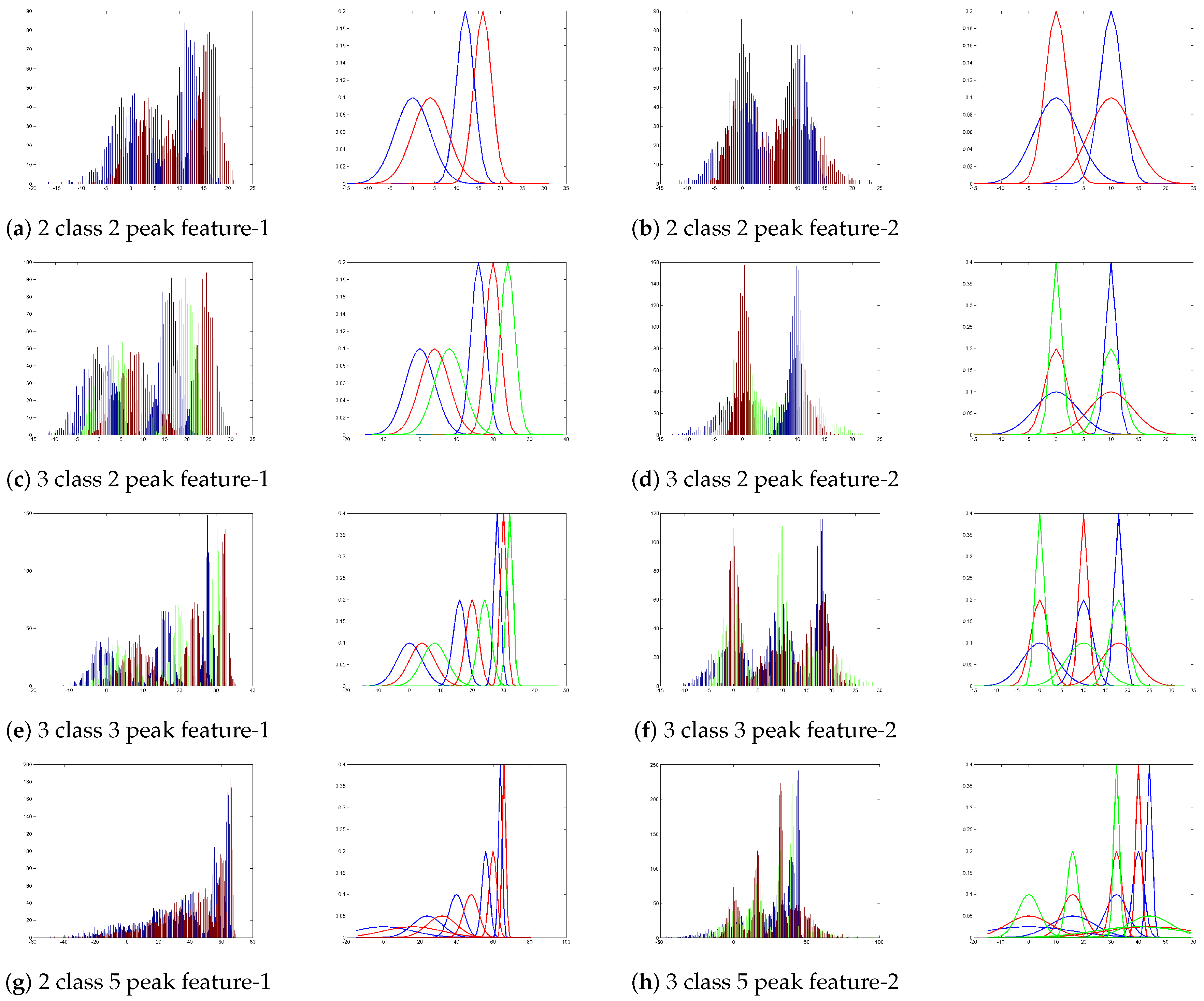
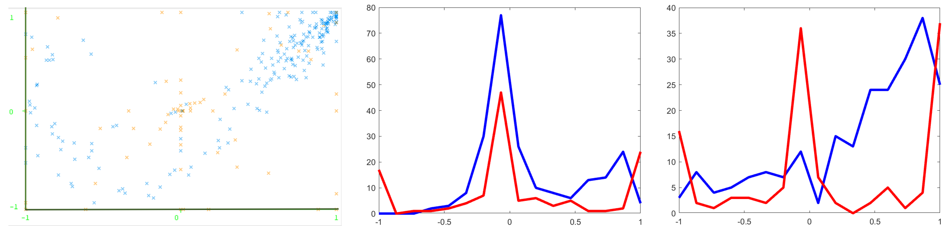
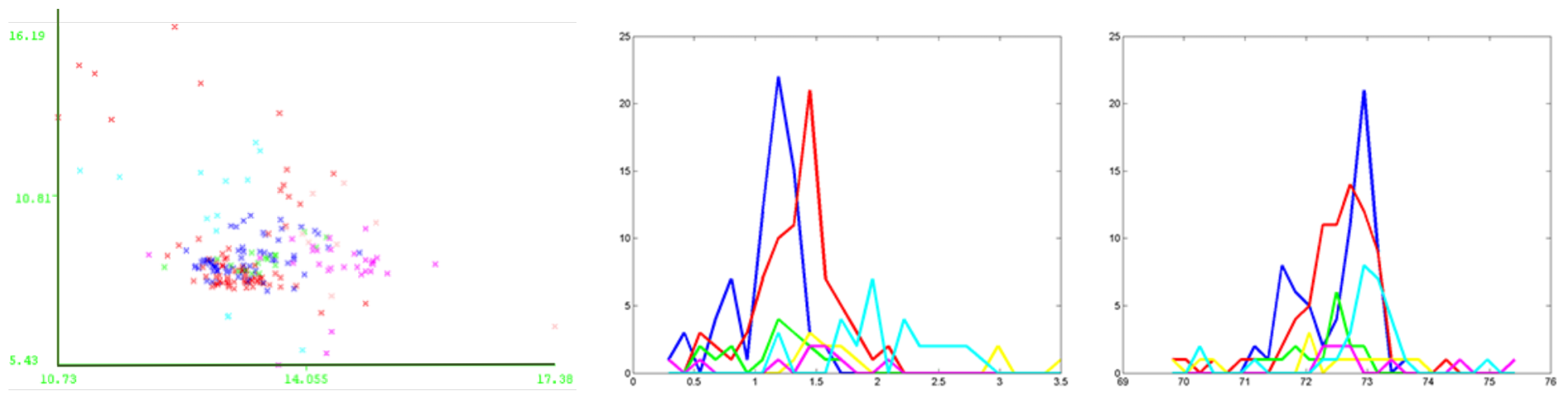
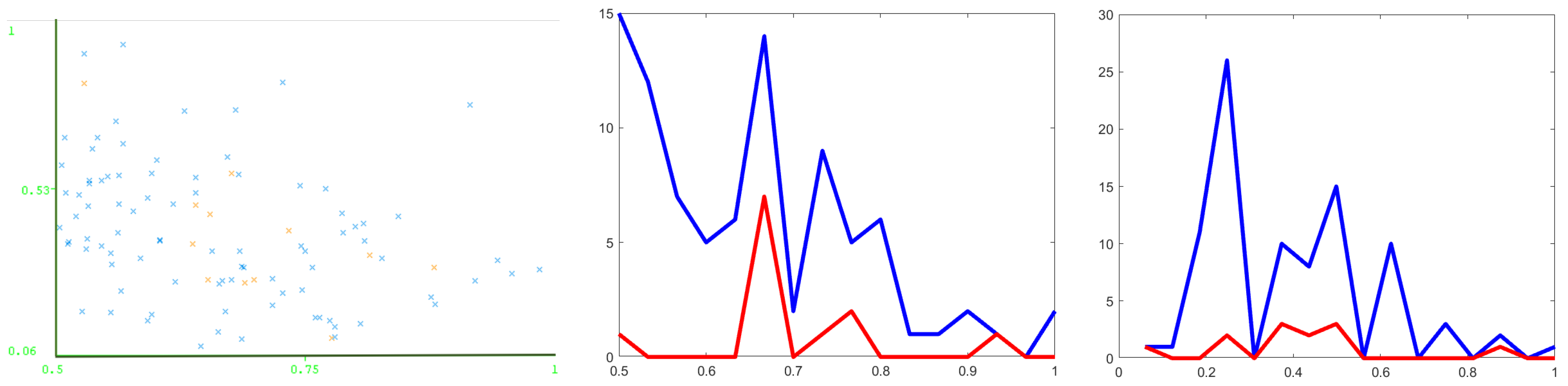
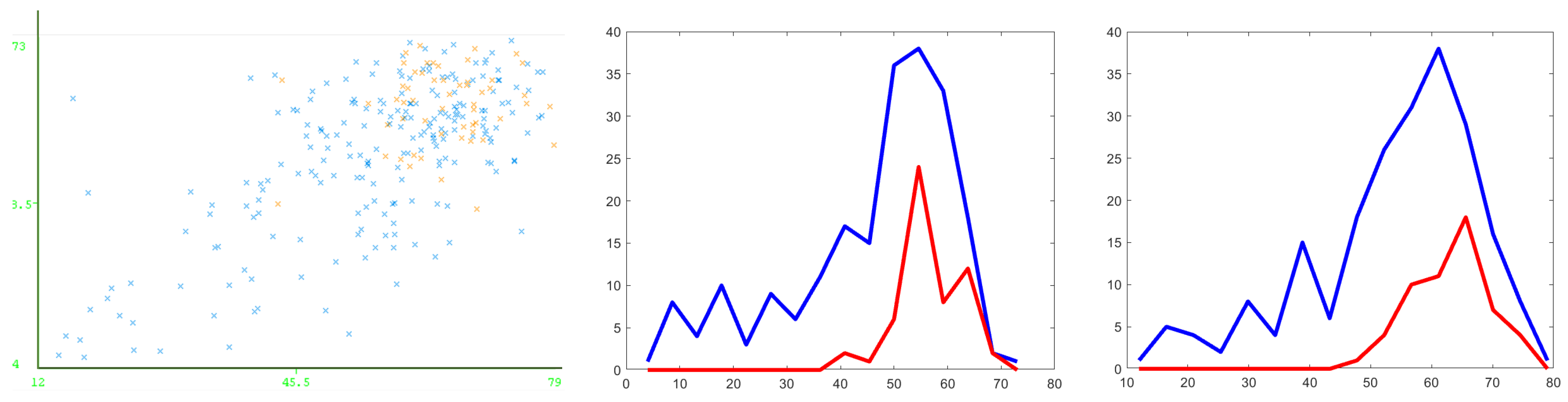
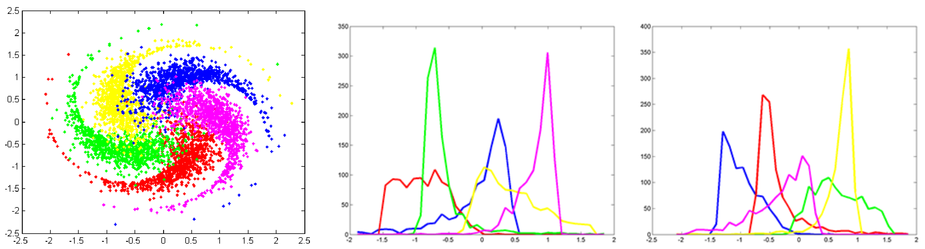
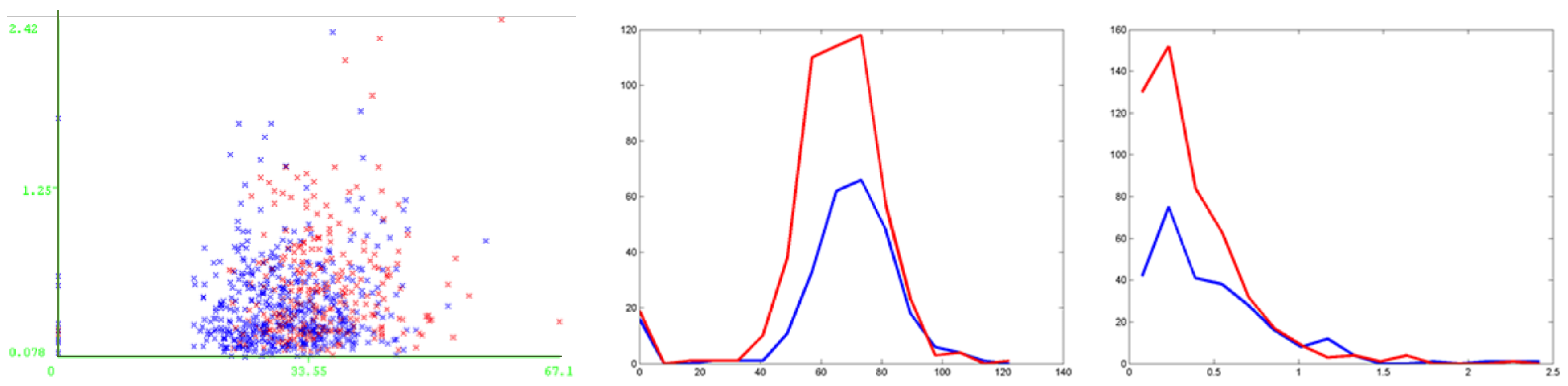
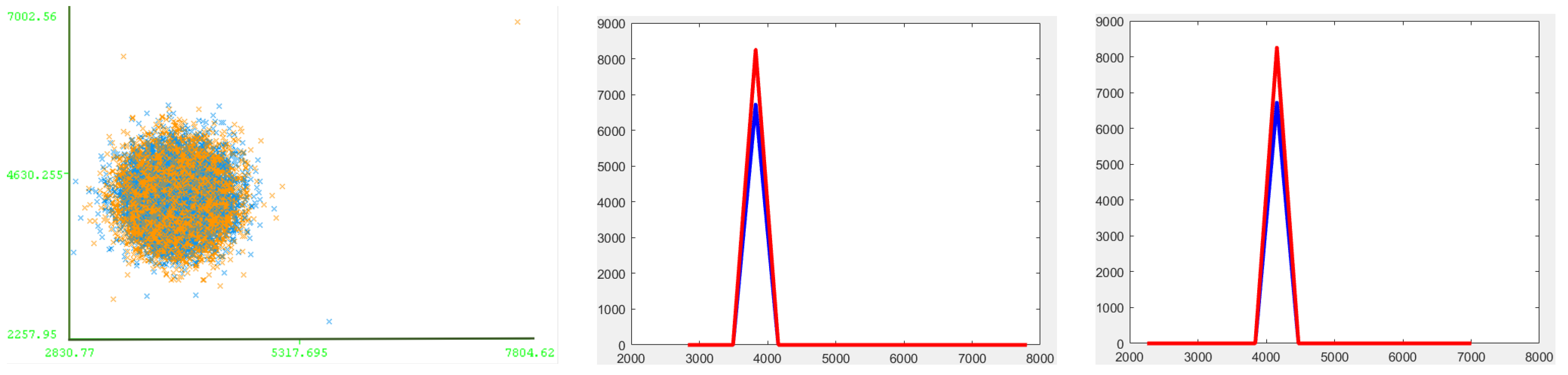
Appendix A. Synthetic and Benchmark Dataset Visualization

Figure A1 visualizes the histogram and distribution of the synthetic dataset. Figure A2, Figure A3, Figure A4, Figure A5, Figure A6, Figure A7 and Figure A8 visualizes scatter and histogram of the benchmark dataset.
Figure A1. Histogram and Distribution of Synthetic Dataset.
Computation 08 00006 g0a1
Figure A2. Scatter and Histogram of Ionosphere Dataset.
Computation 08 00006 g0a2
Figure A3. Scatter and Histogram of Glass Dataset.
Computation 08 00006 g0a3
Figure A4. Scatter and Histogram of Fertility Dataset.
Computation 08 00006 g0a4
Figure A5. Scatter and Histogram of SPECTF Dataset.
Computation 08 00006 g0a5
Figure A6. Scatter and Histogram of Pinwheel Dataset.
Computation 08 00006 g0a6
Figure A7. Scatter and Histogram of Pima Dataset.
Computation 08 00006 g0a7
Figure A8. Scatter and Histogram of EEG Dataset.
Computation 08 00006 g0a8

References

  1. Baltrušaitis, T.; Ahuja, C.; Morency, L.P. Multimodal machine learning: A survey and taxonomy. IEEE Trans. Pattern Anal. Mach. Intell. 2018, 41, 423–443. [Google Scholar] [CrossRef] [PubMed] [Green Version]
  2. Poria, S.; Cambria, E.; Hussain, A.; Huang, G.B. Towards an intelligent framework for multimodal affective data analysis. Neural Netw. 2015, 63, 104–116. [Google Scholar] [CrossRef] [PubMed]
  3. Atrey, P.K.; Hossain, M.A.; El Saddik, A.; Kankanhalli, M.S. Multimodal fusion for multimedia analysis: A survey. Multimed. Syst. 2010, 16, 345–379. [Google Scholar] [CrossRef]
  4. Corneanu, C.A.; Simón, M.O.; Cohn, J.F.; Guerrero, S.E. Survey on rgb, 3d, thermal, and multimodal approaches for facial expression recognition: History, trends, and affect-related applications. IEEE Trans. Pattern Anal. Mach. Intell. 2016, 38, 1548–1568. [Google Scholar] [CrossRef] [PubMed] [Green Version]
  5. Soleymani, M.; Garcia, D.; Jou, B.; Schuller, B.; Chang, S.F.; Pantic, M. A survey of multimodal sentiment analysis. Image Vis. Comput. 2017, 65, 3–14. [Google Scholar] [CrossRef]
  6. Kumar, A.; Kim, J.; Cai, W.; Fulham, M.; Feng, D. Content-based medical image retrieval: A survey of applications to multidimensional and multimodality data. J. Digit. Imaging 2013, 26, 1025–1039. [Google Scholar] [CrossRef] [Green Version]
  7. Oskouie, P.; Alipour, S.; Eftekhari-Moghadam, A.M. Multimodal feature extraction and fusion for semantic mining of soccer video: A survey. Artif. Intell. Rev. 2014, 42, 173–210. [Google Scholar] [CrossRef]
  8. Abidi, B.R.; Aragam, N.R.; Yao, Y.; Abidi, M.A. Survey and analysis of multimodal sensor planning and integration for wide area surveillance. ACM Comput. Surv. (CSUR) 2009, 41, 7. [Google Scholar] [CrossRef]
  9. Kiela, D.; Grave, E.; Joulin, A.; Mikolov, T. Efficient large-scale multi-modal classification. In Proceedings of the Thirty-Second AAAI Conference on Artificial Intelligence, New Orleans, LA, USA, 2–7 February 2018. [Google Scholar]
  10. Vortmann, L.M.; Schult, M.; Benedek, M.; Walcher, S.; Putze, F. Real-Time Multimodal Classification of Internal and External Attention. In Proceedings of the Adjunct of the 2019 International Conference on Multimodal Interaction, Suzhou, China, 14–18 October 2019; p. 14. [Google Scholar]
  11. Zhang, D.; Wang, Y.; Zhou, L.; Yuan, H.; Shen, D.; Alzheimer’s Disease Neuroimaging Initiative. Multimodal classification of Alzheimer’s disease and mild cognitive impairment. Neuroimage 2011, 55, 856–867. [Google Scholar] [CrossRef] [Green Version]
  12. Molina, J.F.G.; Zheng, L.; Sertdemir, M.; Dinter, D.J.; Schönberg, S.; Rädle, M. Incremental learning with SVM for multimodal classification of prostatic adenocarcinoma. PLoS ONE 2014, 9, e93600. [Google Scholar]
  13. Ortiz, A.; Munilla, J.; Gorriz, J.M.; Ramirez, J. Ensembles of deep learning architectures for the early diagnosis of the Alzheimer’s disease. Int. J. Neural Syst. 2016, 26, 1650025. [Google Scholar] [CrossRef] [PubMed]
  14. Ma’sum, M.A.; Sanabila, H.; Jatmiko, W. Multi codebook LVQ-based artificial neural network using clustering approach. In Proceedings of the 2015 International Conference on Advanced Computer Science and Information Systems (ICACSIS), Depok, Indonesia, 10–11 October 2015; pp. 263–268. [Google Scholar]
  15. Hartigan, J.A.; Wong, M.A. Algorithm AS 136: A k-means clustering algorithm. J. R. Stat. Society. Ser. C Applied Stat. 1979, 28, 100–108. [Google Scholar] [CrossRef]
  16. McLachlan, G.J.; Basford, K.E. Mixture Models: Inference and Applications to Clustering; Marcel Dekker: New York, NY, USA, 1988; Volume 84. [Google Scholar]
  17. Mirkin, B. Clustering for Data Mining: A Data Recovery Approach; Chapman and Hall/CRC: Boca Raton, FL, USA, 2005. [Google Scholar]
  18. Ruck, D.W.; Rogers, S.K.; Kabrisky, M.; Oxley, M.E.; Suter, B.W. The multilayer perceptron as an approximation to a Bayes optimal discriminant function. IEEE Trans. Neural Netw. 1990, 1, 296–298. [Google Scholar] [CrossRef] [PubMed]
  19. Hinton, G.E.; Osindero, S.; Teh, Y.W. A fast learning algorithm for deep belief nets. Neural Comput. 2006, 18, 1527–1554. [Google Scholar] [CrossRef] [PubMed]
  20. Vincent, P.; Larochelle, H.; Lajoie, I.; Bengio, Y.; Manzagol, P.A. Stacked denoising autoencoders: Learning useful representations in a deep network with a local denoising criterion. J. Mach. Learn. Res. 2010, 11, 3371–3408. [Google Scholar]
  21. Huang, G.B.; Zhu, Q.Y.; Siew, C.K. Extreme learning machine: Theory and applications. Neurocomputing 2006, 70, 489–501. [Google Scholar] [CrossRef]
  22. Fleury, A.; Vacher, M.; Noury, N. SVM-based multimodal classification of activities of daily living in health smart homes: Sensors, algorithms, and first experimental results. IEEE Trans. Inf. Technol. Biomed. 2010, 14, 274–283. [Google Scholar] [CrossRef] [Green Version]
  23. Gomez-Chova, L.; Tuia, D.; Moser, G.; Camps-Valls, G. Multimodal classification of remote sensing images: A review and future directions. Proc. IEEE 2015, 103, 1560–1584. [Google Scholar] [CrossRef]
  24. Gallo, I.; Calefati, A.; Nawaz, S. Multimodal Classification Fusion in Real-World Scenarios. In Proceedings of the 2017 14th IAPR International Conference on Document Analysis and Recognition (ICDAR), Kyoto, Japan, 9–15 November 2017; Volume 5, pp. 36–41. [Google Scholar]
  25. Chambon, S.; Galtier, M.N.; Arnal, P.J.; Wainrib, G.; Gramfort, A. A deep learning architecture for temporal sleep stage classification using multivariate and multimodal time series. IEEE Trans. Neural Syst. Rehabil. Eng. 2018, 26, 758–769. [Google Scholar] [CrossRef] [Green Version]
  26. Kohonen, T. Improved versions of learning vector quantization. In Proceedings of the 1990 IJCNN International Joint Conference on Neural Networks, San Diego, CA, USA, 17–21 June 1990; pp. 545–550. [Google Scholar]
  27. Sato, A.; Yamada, K. Generalized learning vector quantization. In Advances in Neural Information Processing Systems; The MIT Press: London, UK, 1996; pp. 423–429. [Google Scholar]
  28. Setiawan, I.M.A.; Imah, E.M.; Jatmiko, W. Arrhytmia classification using fuzzy-neuro generalized learning vector quantization. In Proceedings of the 2011 International Conference on Advanced Computer Science and Information System (ICACSIS), Jakarta, Indonesia, 17–18 December 2011; pp. 385–390. [Google Scholar]
  29. Rachmadi, M.F.; Ma’sum, M.A.; Setiawan, I.M.A.; Jatmiko, W. Fuzzy learning vector quantization particle swarm optimization (FLVQ-PSO) and fuzzy neuro generalized learning vector quantization (FN-GLVQ) for automatic early detection system of heart diseases based on real-time electrocardiogram. In Proceedings of the 2012 SICE Annual Conference (SICE), Akita, Japan, 20–23 August 2012; pp. 465–470. [Google Scholar]
  30. Parisi, G.I.; Tani, J.; Weber, C.; Wermter, S. Emergence of multimodal action representations from neural network self-organization. Cogn. Syst. Res. 2017, 43, 208–221. [Google Scholar] [CrossRef] [Green Version]
  31. Lu, D.; Popuri, K.; Ding, G.W.; Balachandar, R.; Beg, M.F. Multimodal and Multiscale Deep Neural Networks for the Early Diagnosis of Alzheimer’s Disease using structural MR and FDG-PET images. Sci. Rep. 2018, 8, 5697. [Google Scholar] [CrossRef] [PubMed] [Green Version]
  32. Kusumoputro, B.; Budiarto, H.; Jatmiko, W. Fuzzy-neuro LVQ and its comparison with fuzzy algorithm LVQ in artificial odor discrimination system. ISA Trans. 2002, 41, 395–407. [Google Scholar] [CrossRef]
Figure 1. Multi-modal Representations.
Computation 08 00006 g001
Figure 2. The LVQ architecture.
Computation 08 00006 g002
Figure 3. The FNGLVQ architecture illustration.
Computation 08 00006 g003
Figure 4. Idea of Multicodebook Approach.
Computation 08 00006 g004
Figure 5. Multicodebook FNGLVQ Architecture.
Computation 08 00006 g005
Figure 6. The impact of number of cluster on K-Means clustering.
Computation 08 00006 g006
Figure 7. The impact of number of cluster on GMM Clustering.
Computation 08 00006 g007
Figure 8. The impact of prunning on K-Means Clustering.
Computation 08 00006 g008
Figure 9. The impact of prunning on GMM Clustering.
Computation 08 00006 g009
Figure 10. Best Accuracy.
Computation 08 00006 g010
Figure 11. Best Number of Cluster.
Computation 08 00006 g011
Figure 12. Result of Incremental Learning.
Computation 08 00006 g012
Table 1. Detail of datasets.
No.Dataset#Features#Instances#ClassesSource
12Peak-2Class54.0002Synthetic
22Peak-3Class56.0003Synthetic
32peak-5Class510.0005Synthetic
43Peak-2Class56.0002Synthetic
53Peak-3Class59.0003Synthetic
63peak-5Class515.0005Synthetic
75Peak-2Class510.0002Synthetic
85Peak-3Class515.0003Synthetic
95peak-5Class525.0005Synthetic
10Glass92146UCI
11Ionosphere333512UCI
12Fertility612994UCI
13Pima131753UCI
14SPECTF510004UCI
15Pinwheel250005-
16EEG25404UCI
Table 2. FNGLVQ Setup parameters.
AlphaBethaGammaAccuracy
0.10.000050.0000575.175
0.10.000050.0000171.325
0.10.000010.0000575.175
0.10.000010.0000175.175
0.050.000050.0000578.78
0.050.000050.0000174.22
0.050.000010.0000578.78
0.050.000010.0000174.22
Table 3. Comparison on Synthetic Dataset.
DatasetLVQ2-1GLVQFNGLVQMC
FNGLVQ
GMM
MC
FNGLVQ
KMeans
MC
FNGLVQ
IL
MLPSAEDBNELM
2peak-2class75.3776.8078.7885.2085.4084.8381.5075.7876.8053.52
2peak-3class67.1268.2562.5186.8287.2383.9278.2067.5270.6351.56
2peak-5class44.5837.3746.2676.0274.6558.8767.1031.7237.5423.77
3peak-2class78.1882.6177.5391.5590.9889.0787.6081.8782.8353.61
3peak-3class63.2460.8758.1488.0288.6381.7274.5359.5766.4336.75
3peak-5class41.8835.5035.6477.3776.8867.4651.5133.7735.0331.62
5peak-2class73.6477.2177.5990.6088.7774.2885.0276.8178.2838.33
5peak-3class54.9767.0360.4985.2981.6368.6876.8068.7278.7839.63
5peak-5class40.9949.8441.0481.9680.8354.9863.6159.8961.4121.31
Average 2peak62.3660.8162.5282.6882.4375.8775.6058.3461.6642.95
Average 3peak61.1059.6657.1085.6585.5079.4271.2158.4061.4340.66
Average 5peak56.5364.6959.7185.9583.7465.9875.1468.4772.8233.09
Average all60.0061.7259.7884.7683.8973.7573.9961.7465.3138.90
Table 4. Comparison on Benchmark Dataset.
DatasetLVQ2-1GLVQFNGLVQMC
FNGLVQ
GMM
MC
FNGLVQ
KMeans
MC
FNGLVQ
IL
MLPSAEDBNELM
Ionosphere83.7687.7585.4791.7492.5993.4490.3164.0087.4387.43
Glass55.1464.0056.0060.3462.1965.0559.3436.6712.8648.10
Fertility86.0087.0087.0088.0888.0083.9784.0058.0088.0083.00
Pima66.8863.6771.0949.7572.5270.9676.2375.5565.1066.01
SPECTF79.4067.3979.4079.4080.5279.7478.2880.0080.7579.62
Pinwheel92.2287.7892.0496.3296.2099.6289.5423.4895.8098.44
EEG59.9349.4255.2157.7767.5853.0653.0651.0955.1255.12
Average74.7672.4375.1777.6079.9477.9875.8255.5469.2973.96
Table 5. Scoring.
Table 5. Scoring.
DatasetLVQ2-1GLVQFNGLVQMC
FNGLVQ
GMM
MC
FNGLVQ
KMeans
MC
FNGLVQ
IL
MLPSAEDBNELM
2peak-2class25691087351
2peak-3class35291087461
2peak-5class53610978241
3peak-2class35210987461
3peak-3class54291087361
3peak-5class64510987231
5peak-2class25610938471
5peak-3class24310957681
5peak-5class24310958671
Ionosphere26389107154
Glass49578106213
Fertility57710934192
Pima52718610934
SPECTF51559728106
Pinwheel52487103169
EEG81710944266
Average Score4.004.194.568.508.946.886.383.635.752.69

