Particulate Matter and COVID-19 Disease Diffusion in Emilia-Romagna (Italy). Already a Cold Case?


Department of Computer Science and Engineering, University of Bologna, 40127 Bologna, Italy
*
Author to whom correspondence should be addressed.
Computation 2020, 8(2), 59; https://0-doi-org.brum.beds.ac.uk/10.3390/computation8020059
Submission received: 11 May 2020
/
Revised: 14 June 2020
/
Accepted: 19 June 2020
/
Published: 23 June 2020
(This article belongs to the Special Issue Computation to Fight SARS-CoV-2 (CoVid-19))
Abstract
:As we prepare to emerge from an extensive and unprecedented lockdown period, due to the COVID-19 virus infection that hit the Northern regions of Italy with the Europe’s highest death toll, it becomes clear that what has gone wrong rests upon a combination of demographic, healthcare, political, business, organizational, and climatic factors that are out of our scientific scope. Nonetheless, looking at this problem from a patient’s perspective, it is indisputable that risk factors, considered as associated with the development of the virus disease, include older age, history of smoking, hypertension and heart disease. While several studies have already shown that many of these diseases can also be favored by a protracted exposure to air pollution, there has been recently an insurgence of negative commentary against authors who have correlated the fatal consequences of COVID-19 (also) to the exposition of specific air pollutants. Well aware that understanding the real connection between the spread of this fatal virus and air pollutants would require many other investigations at a level appropriate to the scale of this phenomenon (e.g., biological, chemical, and physical), we propose the results of a study, where a series of the measures of the daily values of PM2.5, PM10, and NO2 were considered over time, while the Granger causality statistical hypothesis test was used for determining the presence of a possible correlation with the series of the new daily COVID19 infections, in the period February–April 2020, in Emilia-Romagna. Results taken both before and after the governmental lockdown decisions show a clear correlation, although strictly seen from a Granger causality perspective. Moving beyond the relevance of our results towards the real extent of such a correlation, our scientific efforts aim at reinvigorating the debate on a relevant case, that should not remain unsolved or no longer investigated.
1. Introduction
Although COVID-19 has originated in Wuhan, China in late 2019, several provinces of northern Italy have soon become among the hardest-hit regions in Europe. This virus outbreak spread with a particular intensity to the Italian regions of Lombardy, Veneto, Emilia-Romagna, and Piedmont, in the period from late February to late April, with a severe toll in terms of human deaths. As a simple evidence of this disaster, it suffices to remind that the Italian Institute of Statistics (ISTAT) has recently computed for Italy an average increase of 49.4% in the number of all the fatalities occurred during the month of March 2020, as compared with the number of deaths of March 2019 [1]. Not to mention that, in the same month of March 2020, the official death toll, for some given provinces, like Bergamo and Brescia (in Lombardy), stands at more than five times the value recorded one year before, same period [1].
While it is true that Italy had the bad luck of being the first European country to be devastated by the outbreak, what has gone wrong has motivations in a combination of demographic, political, organizational, industrial, climatic factors, and low intensive care unity (ICU) capacity as well, that need further specific investigations.
Nonetheless, while we are aware that what went wrong will be a subject of studies for years, we are concerned, here, with the fact that COVID-19 manifests as a severe respiratory disease, mostly pneumonia. This motivates why many researchers have focused their attention on the potential relationship between the exposure to particulate pollution and the rapid contagion brought by this virus. With this in view, recently, many international scientific studies were developed to investigate the relationship between particulates of various types and the COVID-19 incidence.
Exemplar is the work by Jiang, Wu and Guan that addresses two relevant issues, with reference to the association between particulate and COVID-19 [2]. They start from the very general consideration that air pollutants raise concerns over their association with infectious diseases, being often the cause of local epidemics [3,4]. This is typical with influenza, since the airborne air pollutants perform as condensation nuclei for the virus to attach, as also confirmed by several other studies [5,6,7,8,9]. Owing to this consideration, Jiang et al. proceed with the following reasoning: since COVID-19 is known to cause human-to-human transmission by infectious secretions [10], these secretions could be transferred in many different ways, including ambient air pollutants. Not only, Jiang, Wu and Guan also observe that is not by chance that PM2.5 is the air pollutant constantly associated with an increased COVID-19 incidence in all the Chinese cities of their study, namely: Wuhan, XiaoGan, and HuangGang. Besides the fact that particulate could provide condensation nuclei for viral attachment, Jiang, Wu and Guan add a second biomedical argument which is as follows. It has been discovered that the receptor for COVID binding is the angiotensin-converting enzyme 2, that concentrates on the type II alveolar cells [11]. Since, type II alveolar cells are located in the alveoli, which are only reachable to particles with diameters less than 5 micro meters, it becomes evident that very small airborne pollutants, such as PM2.5, have the potential to penetrate, unfiltered, the respiratory tract, down to the alveolar region [12,13,14,15].
Similarly, interesting results were found also by Pansini and Fornacca who investigated the incidence of COVID-19 mortality rate in highly polluted areas. They focused their attention on selected areas from different countries (including, among others, China, Italy, and US), and considered also CO and NO2, in addition to particulates. In particular, they collected data about air quality from two kinds of sources: ground monitoring stations and satellite. According to the analysis they performed, they found significant positive correlations between COVID-19 infections and air quality variables. Yet, while in China the strongest correlation was found with the (satellite-derived) CO values, in Italy and in the US the highest correlation values, with the incidence of COVID-19, were those of NO2, derived respectively from satellite (Italy) and ground measurements (US). One of their final observation is that the COVID-19 mortality ratio is higher, regardless of the higher number of infections, in all those areas with poor air quality, that is, where values of CO, NO2, and PM are constantly higher than the acceptable limits [16].
Nevertheless, besides this set of international studies developed in this field (the interested reader can refer also to [17,18]), we scrutinized, with special interest, just those recently conducted by members of the Italian scientific community, for two main reasons. First, the impact of particulate pollution was already being severely felt as a huge health problem in Northern Italy, well before the advent of COVID19 and, second, those studies have been put at the centre of a heated debate in Italy, and considered not convincing under different perspectives.
To be precise, (almost) all those papers at the centre of this controversy have followed two concurrent lines of reasoning, that are typical when one wishes to infer causal relations from data. On one side, they have tried to acquire (through experimentation) the knowledge of the biological/chemical/physical mechanisms at the basis of the possible correlation between the particulate and the virus spread. On the other side, they have tried to confirm the existence of a true causal relation between the two aforementioned phenomena, using some kind of statistical hypothesis testing.
The works conducted by Setti et al., for example, provided a quite convincing contribution to this discussion, by both revealing that traces were found of the COVID-19 RNA in PM10 samples in Bergamo [19], and also testing the hypothesis of such a correlation between the daily surplus of that particulate and the consequent contagion between humans by exploiting the statistical model of the coefficient of determination [20]. Daily infections were recorded in the period from 24 February to 13 March, while a surplus of PM10 values was considered, on a daily basis, in the period from 9 February to 29 February.
Conticini, Frediani, and Caro, instead, without any statistical testing activity in support of their hypothesis, argued about the fact that poor air quality can lead to a state of permanent body inflammation and chronic respiratory difficulties, along with a hyper-activation of the immune system; being these all circumstances that makes human lungs prone to be attacked by the virus. This is their hypothesis explaining the high mortality rate, recorded in Emilia-Romagna and Lombardy, owing to the virus outbreak [21].
Finally, Becchetti et al. analysed both the PM10 and PM2.5 values, although recorded on an annual basis, and correlated them to COVID-19 infections and mortality, using a cross-sectional regression statistical method. Theirs is a vast study, where scrutinized are also other factors, including temperature, population density, income, number of lung ventilators, and public transport usage. Nonetheless, the conclusion is that air pollution can be considered as a strong predictor for both virus contagions and mortality [22]. In that paper, again, cited as mechanisms at the basis of the correlation between the particulate pollution and the contagion are, respectively, the hypotheses that: (i) humans living in highly polluted areas have a reduced respiratory capacity to react to the virus, and (ii) the particulate may act as a carrier for the virus.
Unfortunately, all these papers have been severely criticized, mostly based on the considerations that they did not contain any robust evidence of the aforementioned correlation, and that all those discoveries boil down to vague clues, completely preliminary, not yet subject to peer-review by experts in the field [23].
Far from taking a final position, we hold the firm view that all the authors we have cited before share, at least, the merit of having tried to inquire into a vexed problem, that should not go unsolved, or no longer investigated, until a final solution is found.
Hence, our contribution, here, is to provide a further investigation on the possibility that a causal correlation exists between the two cited phenomena (i.e., pollution and spread of the infections). We, as investigators, have to admit that we do not possess any prior knowledge of the researched correlation at a level appropriate to the scale of this phenomenon, e.g., biological, chemical, and physical, and we want to limit our study to an examination of the plausibility of the existence of that correlation at a statistical level. In particular, we are interested in verifying if that correlation comes either confirmed (or rejected) using an alternative statistical model, namely the Granger-causality hypothesis testing model.
Specifically, the Granger causality test is a statistical hypothesis test where a time series X is said to Granger cause Y, if it can be shown, through a series of statistical tests on lagged values of X, that those X values provide statistically significant information about future values of Y. To this aim, it is worth mentioning that we analysed the daily values of the following air pollutants: PM2.5, PM10, and NO2, treated as time series occurring in a given temporal period that has preceded the series of the COVID-19 infections, in all the provinces of the Emilia-Romagna region.
Finally, it is also worth mentioning that we know very well that many believe that some results of the Granger-causality tests can often have a low epistemic utility. Especially, in specific situations when the theoretical background behind the cause–effect correlation is insufficient, or the validation experiments on the field have not been yet conducted. Though, we will argue that the results of our tests, obtained both before and after the Italian government lockdown decisions taken on 8–10 March, posit the correlational structure between pollution and infections well beyond the limit of a weak Humean interpretation of causality [24], with possible implications of practical relevance. Nevertheless, our study does not have to be treated as the final proof a true causality nexus between the two phenomena, but as an additional strong clue on a case that does not deserve to be already archived.
2. Methods
We now present some preliminary information relevant to our study and a description of the data we have used, along with some reflections on the statistical methodology we have employed.
2.1. Preliminary Information
As already anticipated, in this study we are interested in reasoning around the plausibility of a correlation between air pollution and the spread of COVID-19 infections in the Emilia-Romagna region, by subjecting such hypothesis to a statistical hypothesis testing from a Granger-causality perspective.
Prior to beginning, it is important to make clear that we have taken into considerations all the provinces of the Emilia-Romagna region, in the period of interest, namely: Bologna, Ferrara, Forlì-Cesena, Modena, Parma, Piacenza, Reggio nell’Emilia, Rimini, and Ravenna. It is worth mentioning that this Italian region is populated by almost 4,500,000 citizens and has been one of the more seriously affected by this virus, with a total number of infections of 26,719, and as many as 3827 fatalities, as of 9 May 2020.
Of paramount importance to view this process from the right temporal perspective, there are also to consider the events of the chronology according to which restrictions were imposed to human activities in those provinces (with the aim of slowing down the infective diffusion). In particular:
2.2. Data Description
The data on which we performed testing activity were essentially of two types: i) the time series relative to the new daily COVID-19 infections, and ii) the air pollution In Emilia-Romagna, under the form of the measurements of the following pollutants: PM2.5, PM10, and N02, taken on a daily basis at all the aforementioned provinces (Bologna, Ferrara, Forlì-Cesena, Modena, Parma, Piacenza, Reggio nell’Emilia, Rimini and Ravenna).
The amount of daily infections was collected using the GitHub repository of the Italian Civil Protection, for the entire period starting on 24 February and closing on 17 April 2020 [27].
The daily values of the pollutants mentioned before, instead, were collected using the website of the Regional Environmental Protection Agencies (ARPA) of the Emilia-Romagna region, for all the nine provinces we have cited before [28]. Since there were multiple monitoring stations distributed over each province, an average of the values returned by each station was computed, on a daily, provincial basis.
More important is what follows. We have all learnt that this COVID-19 infection can be subjected to an incubation period, whose duration can range from a few days to almost 14, before an infected human begin to manifest some given symptoms. More precisely, authors of [29] maintain that the median incubation period can be estimated to be 5.1 days (with a confidence interval of 95%, it takes from 4.5 to 5.8 days), and that the 97.5% of those who develop symptoms will do so within 11.5 days (with a confidence interval of 95%, it takes from 8.2 to 15.6 days). These estimates imply, at the end, that the 99% of the infected population will develop symptoms within 14 days. Further, other authors also emphasize that a spare delay of 3.6 days can be experienced from the moment in time the result of a virological test is performed, and the time when it is recorded in the correspondent database [30].
These are the reasons why we designed the two different time series:
- the one with the average daily pollution values (say X), and the one with the number of the new daily infections (say Y).
- where X was anticipated in time with respect to Y of 14 days. We decided not to use an offset of sixteen days (as resulting from the sum of 12.5 with 3.6) between (a) and (b), simply because this minimum time difference lag was absorbed by the specific statistical methodology we have employed (i.e., the Granger causality), where we have varied the so-called lag length parameter in a range from 3 to 8 days (as better explained in the Section 2.4 below) [31].
Following this reasoning, the period when me measured the particulate (specifically, PM2.5, PM10, and NO2) started on 10 February and closed on 3 April 2020. As already told, instead, the period for measuring the infections was: 24 February–17 April 2020.
Hence, at the end, it should be clear that an offset has been put that temporally separates these two time-series, due to the consideration that all what can happen on a given day, say x, may have its effect in terms of manifestations of the infection after a period in time which can be as long as x + 14 days.
For the sake of conciseness, we have moved the three Figures, with all the twenty-seven graphs showing how our time-series (PM2.5, PM10, and NO2 vs. infections) evolve in time to the Appendix A at the end of this paper.
2.3. Methodology
As already mentioned, we have employed a Granger causality testing model to study if a causal correlation may exist between particulate matter and the spread of new COVID-19 infections in Emilia-Romagna [16].
This is a statistical hypothesis testing model typically used to determine if there is a causal relationship between two time-series. In particular, a time series X is said to Granger-causes a time series Y if the prediction of the nth value of Y, using both the past values of X and Y, provides more information rather than the prediction based only on past values of Y [32].
This model typically rests upon two axioms. The former is that past and present may cause the future, but future cannot cause the past. The latter is that the cause contains a unique information about its effects. Usually, the null hypothesis of such a test is set to the fact that the time series X does not Granger cause the time series Y, while, consequently, the unique alternative hypothesis is that the time series X Granger causes the time series Y.
In our study, the alternative hypothesis was that the pollutants’ time series Granger causes the time-series of the infections. Hence, our aim has been that to verify if we could reject the opposite null hypothesis (i.e., pollution does not Granger cause infections), based on the available data.
To this aim, we set the level of significance at 5%, hence preparing to reject the null hypothesis, only in the case that the corresponding p-values came less than 0.05. Further, as the test assumes that both the time-series under investigation should be stationary, we check and found this condition satisfied using the well-known augmented Dickey–Fuller method [33].
Not only. Since we have designed two time-series where the former (X = pollution) temporally precedes the latter (Y = infection), we did not need to check if the infection Granger causes the pollution, given that the time precedence of Y by X comes naturally.
Nonetheless, it is important to repeat, here again, a concept we have already anticipated in the Introduction. Neither the Granger causality method, nor any other statistical test can provide a final and convincing evidence that two phenomena are correlated, from an epistemological viewpoint, if one has neither a clear knowledge of the motivation that causes that relationship, nor has developed sufficient experiments at a scale that should be appropriate to the observed phenomena.
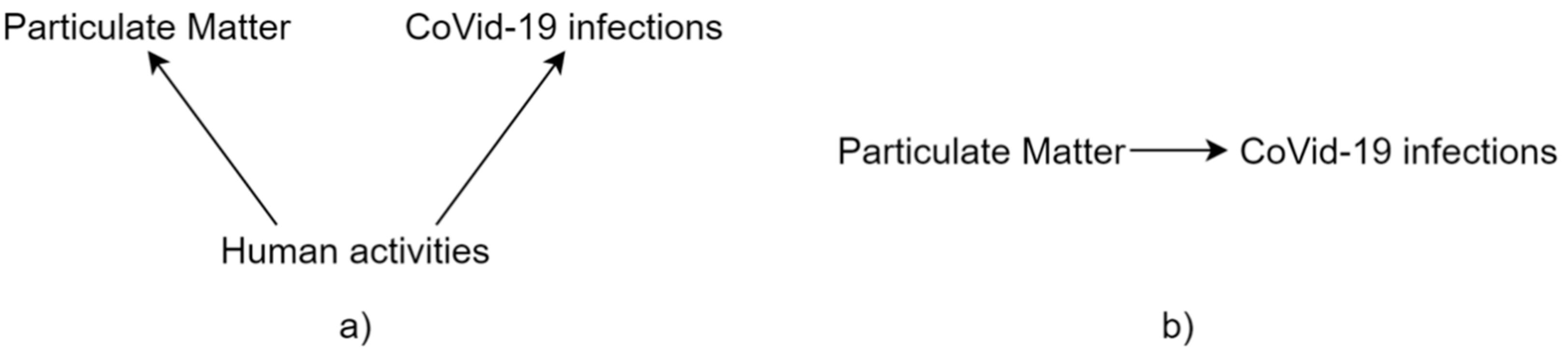
With this regard, the Granger causality approach suffers from an additional problem. In fact, if both X and Y are driven by a common third process, say W, one might still accept the alternative hypothesis of Granger causality (X Granger causes Y), even though it is evident that both X and Y have a common cause (i.e., W), that determines their mutual correlation [34].
Moving this argument at the center of our specific case, one could even argue that the human activities (playing the role of W, here) have been the common basis for the correlation between pollution and infections (as portrayed in Figure 1a) and, hence, a true causality relation between pollution and infection could not be demonstrated, even when our alternative hypothesis is accepted. Nonetheless, in the next section, we will show results, taken both before and after the lockdown decisions (when almost all human activities were at a minimum), that do seem to confirm the existence of a causal structure similar, instead, to that shown in Figure 1b.
2.4. A Computational View
To better understand how a Granger causality testing model works from a computational perspective, fundamental is the following explanation.
We start from two time series X and Y (i.e., pollution and infections), whose causal relationship is to be either demonstrated or rejected. In other words, X and Y are the time series under investigation that can be modeled with the following Granger causality equation:
Specifically, Yt and Xt are the single elements of the two series Y and X, and, in our case, they correspond to the values that Y and X can take on, on a daily basis. In essence, with the formula above we can compute current values of Y, based on previous values of both X and Y. How far back one can go with previous values of X and Y, to perform the computation of the current value of Y, is given by the value of L, the so-called lag. To complete the formula, is a white-noise-random vector.
This said, now comes the turn of explaining how to use this formula for performing a Granger causality hypothesis testing. To this aim, crucial is the role of the coefficients. In fact, we can say that X Granger-causes Y only if the coefficients are not zero, since only in this case past values of X (and Y) become useful to compute current values of Y. On the contrary, coefficients equal to zero make a null contribution to the final sum. It is now easy to understand that modelling a causal relationship with the Granger formula amounts to perform a statistical hypothesis test, where the null hypothesis is that all the coefficients are zero:
The alternative hypothesis being, instead, that at least one of the coefficients is different from zero.
From a computational perspective, at this point, in a case like that of our study, assigned all the actual values for Y and Y, a vector autoregressive procedure (VAR) is to be run to derive the coefficients. Upon computation of those coefficients, a F test procedure must be performed to check if those computed values fit with the all zero distribution of the null hypothesis. This statistical test will return p-values. The higher the returned p-values, the more plausible is the null hypothesis. The lower the p-values, the more plausible is the alternative hypothesis: that is, X Granger causes Y.
Said about the general Granger computational process, now comes the motivation why we have chosen this procedure for our study, rather than other more traditional statistical approaches, like, for the example, the one adopted in [5].
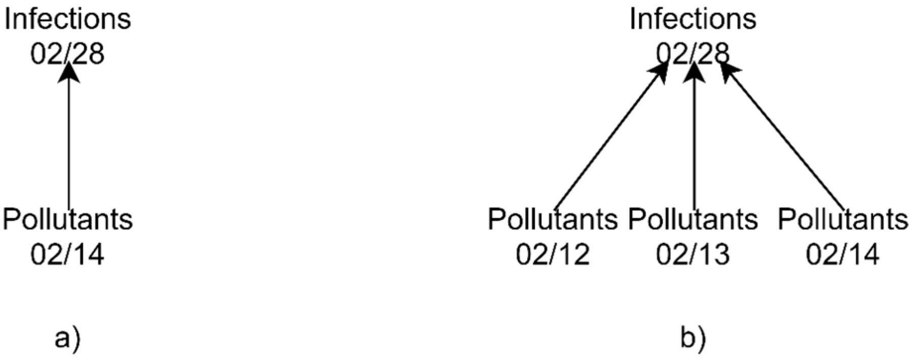
To better understand, consider the following example: Suppose we want to evaluate if a relation exists between the number of viral infections happened in a specific day (e.g., 18 February) and the amount of pollution in the air. To do that, traditional approaches would compute values, based on measurements taken on just two days: the day of the infections vs. the day assumed to be the one when the pollution occurred that was considered at the basis of those infections, say for example February 14th, exactly like in Figure 2a.
With the approach based on the Granger formula, instead, we can take into simultaneous consideration multiple days, each with its amount of measured pollution. This is by virtue of the lag factor (i.e., the L value in the Granger formula above) that allows one to go back as many days as one wants in the computation. For example: three days, like in Figure 2b (or from 3 to 8, like in the case of our study, see Section 2.2).
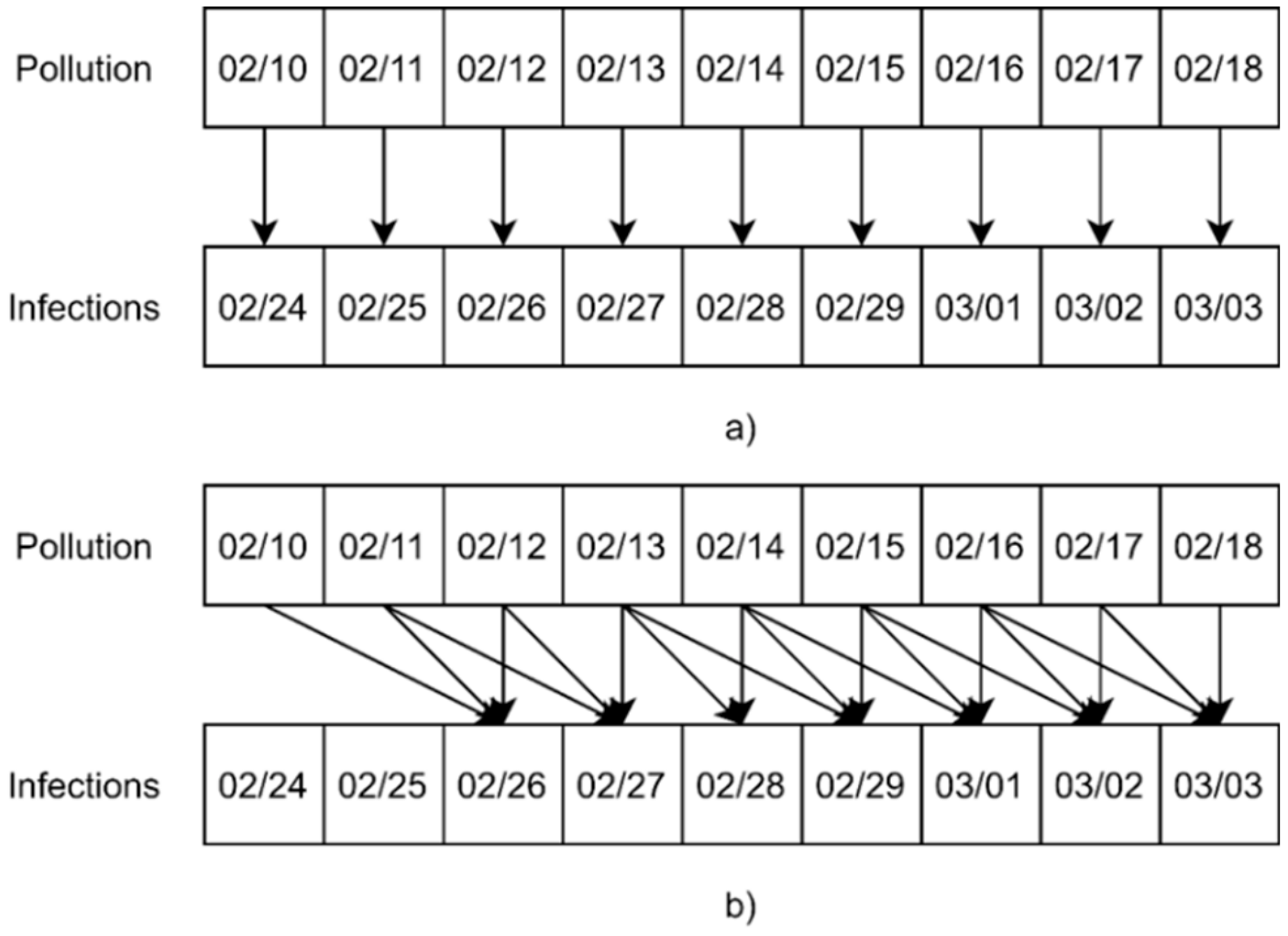
This is a prominent computational aspect that should not go neglected, since the information on when a given infection precisely occurs comes with a large amount of uncertainty. Still more remarkably, since COVID-19 is manifesting with variable temporal dynamics, we should adopt flexible computational methods to study it. From this point of view, as the series shown in Figure 3 comparatively demonstrate, methods like Granger should be preferred, since they hold the promise to analyze simultaneous contributions to the cause of a unique effect.
3. Results
We present the results returned by our Granger causality testing model, differentiating between those illustrating the situation before the lockdown measures were adopted that contained the infection surge, and those showing the ex-post situation.
3.1. Before the Lockdown
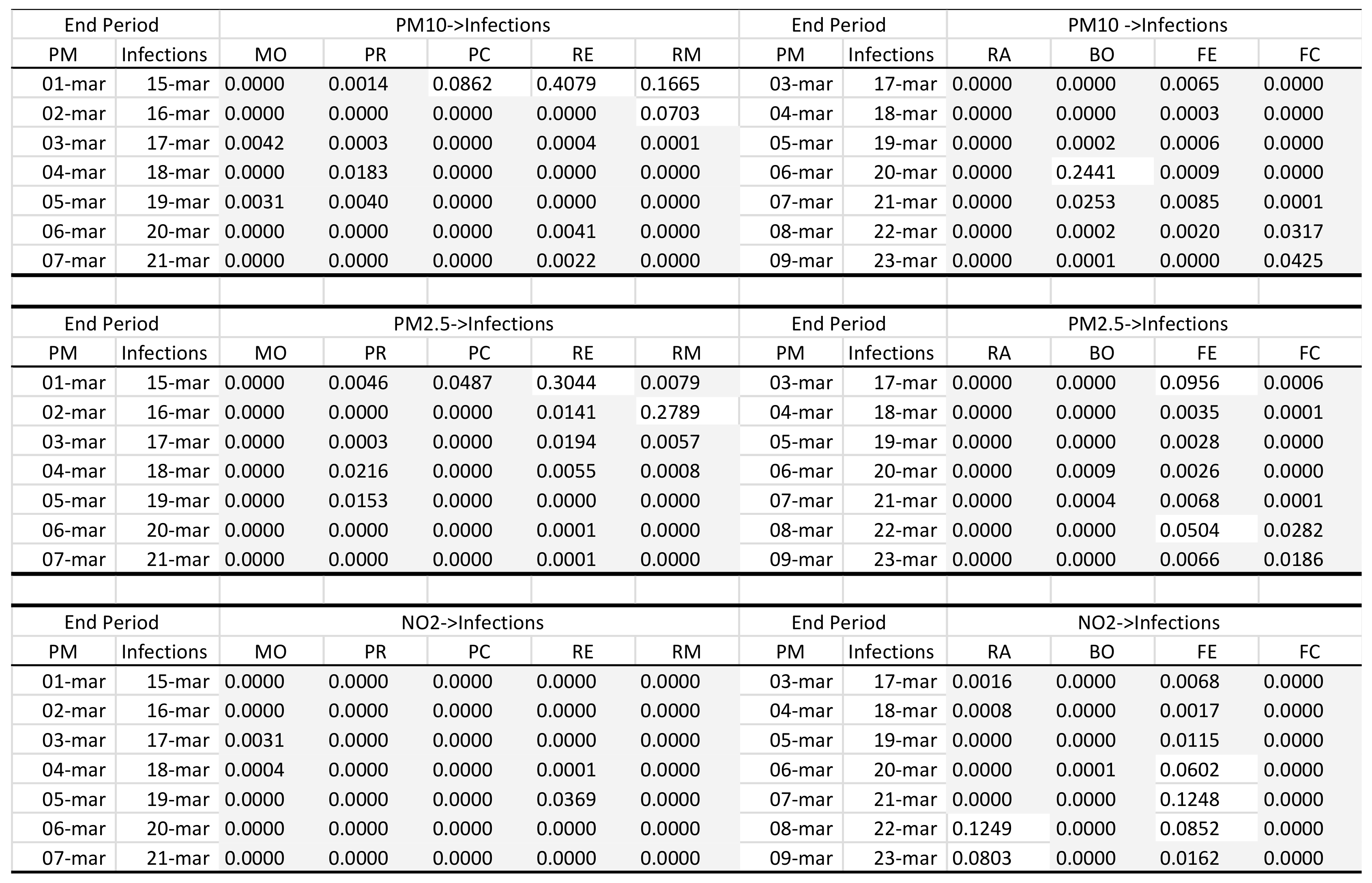
The following Figure 4 reports the results of our Granger causality testing campaign, conducted for all the nine aforementioned provinces of the Emilia-Romagna (Bologna-BO, Ferrara-FE, Forlì-Cesena-FC, Modena-MO, Parma-PR, Piacenza-PC, Ravenna-RA, Reggio nell’Emilia-RE, and Rimini-RM).
As already anticipated, we tried to verify if the series X, comprised of all the average daily values of a given pollutant (e.g., PM2.5), measured in terms of micrograms per cubic meter, starting on day x1 and closing on day x2, Granger causes the series Y of the new daily infections, measured in terms of infected human beings, starting on day y1 and closing on day y2, where obviously: y1 = x1 + 14 and y2 = x2 + 14, for all the days between x1 and x2.
For each of the possible combination pollutant (PM2.5, PM10, and NO2)/infections, our Figure 4 shows in the correspondent cell the p-value obtained through a pairwise series computational comparison, using Granger. All this yields a total amount of 189 pairwise series comparisons. In particular, to read well the results: if a cell in Figure 4 reports a p-value less than 0.005, we have a confirmation of the causality relation between pollutant and infections (finally, note that if a cell in the Figure reports the value of 0, this means that a p-value less than 10−4 was computed).
For an easier comprehension of the Figure, one should also notice that the time scale values reported at the left of Figure 4 are the closing days of the two series (respectively, for pollutants and infections), namely the values termed: x2 and y2.
Precisely, x2 ranges in the Figure from 1 to 7 March or from 3 to 9 March, depending on the specific province under consideration with its correspondent lockdown date (8–10 March), while y2 may range from 15 to 21 March or from 17 to 23 March, due to the 14 days-long temporal shift with which we distanced the two series (pollution precedes infections).
To note, finally, is the fact of prominent importance that all the pairwise series comparisons whose results are reported in Figure 4 were conducted during a period when the lockdown measures were still inactive, since the specific series supposed as the cause of this relation (that is X, the pollutants) starts on 10 February and closes on 7 or 9 March, depending on the province.
All this said, what is clear from an analysis of Figure 4 is that we have got a total amount of 175 (out of 189) statistical confirmations (almost 93%) that X Granger causes Y; that is. that the pollutants under consideration have some effect on the number of new infections, from a Granger-causality perspective. In particular, this correlation is slightly more evident with PM2.5 (yielding 94%), rather than with PM10 and NO2 (92%). Further, to be specified is the fact that there are 189 different pairwise temporal series comparisons, and each was performed with the Granger method explained in Section 2.4.
Nonetheless, before one can come to some final conclusion, we have to remember, here again, the reflection we have anticipated in the previous Section, and that we can repeat, under the alternative form of a question: What about if the human activities carried out in the period from 10 February to 7 or 9 March, were the only common cause for both pollution and infections, exactly like in the causality scheme portrayed in the example a) of Figure 1?
If so, the value of the analysis we have conducted so far would be almost controversial. To respond to this doubt, we ask the reader to refer to the next Subsection.
3.2. After the Lockdown
As already told, the causal modeling method proposed by Granger was designed to handle pairs of variables, and consequently it may suffer from a typical limitation when a third variable is engaged in the relation, as explained in a previous Section. In our specific case, this third variable could be identified with all the variety of human activities that could be the common cause for both the air pollution and the spread of infections in Emilia-Romagna.
Nonetheless, an important factor has come to the scene through which we will try to argue that the relation identified in the previous Subsection still holds. This factor amounts to the lockdown decisions taken either on either 8 or 10 March, depending on the specific province under investigation.
As a result of these decisions, human activities had fallen down to a minimum starting again on either 8 or 10 March, depending on the province under consideration. This has a precise meaning with an impact onto the rationale behind our analysis, which is as follows: All what happens after those dates can no longer be ascribed to the activity carried out by humans (if not minimally).
Nonetheless, looking at this from an opposite perspective, one should also argue that this new factor (i.e., the lockdown) can also have a confusing effect on the researched phenomena, since the absence of humans in the scene could open the way to new unexpected implications, and hence to a variety of different possible interpretations.
To avoid this possible pitfall, we have redesigned our experiments with a specific care to select for our analysis only those provinces whose general characteristics could be considered to be more easily observable, with less external interferences. Two design principles drove us for this new set of experiments. The first was that to exclude from our analysis all those provinces with a too high number of infected individuals per population, with respect to the average value of the region under investigation. This way, Piacenza, Reggio nell’Emilia, Parma and Rimini were excluded, yielding the highest percentages of infected individuals per population, namely: 1.509%, 0.906%, 0.723% and 0.606% (as recorded on 9 May 2020). For an analogous reason, we excluded the largest province in the region, precisely Bologna, since it is suffering a very high number of infected individuals, which are currently as many as 4751. For an opposite motivation, we cut off from the second part of our study also the province of Ferrara, which for a long time, fortunately, had hit the lowest rate of infected individuals per population (even though it has recently recorded higher values, thus reaching currently the percentage of 0.281%).
Finally, excluded went also the province of Forlì-Cesena, in this case due to the fact that we measured a marked decrease in the amount of the values of the particulate measured during the new period of investigation.
To this aim, it is interesting to notice that the difference between the amount of particulate matter taken both before and after the lockdown, computed as an average of the daily measurements of the two two-weeks long periods that preceded and followed the lockdown date, ranged in an interval from +8.65 micrograms per cubic meter (Parma) to –3.33 micrograms per cubic meter (Rimini) for the PM2.5 pollutant, and from +6.30 micrograms per cubic meter (Parma) to –10.47 micrograms per cubic meter (Rimini) for the PM10 pollutant. (At this point, it is also interesting to remind to the reader that the acceptable daily limit considered for PM10 pollutant is set to be 50 micrograms per cubic meter).
All this considered, both the province of Modena and Ravenna were rather stable under this perspective, with incremental values amounting to: +7.86 (PM22.5) and +6.11 (PM2.5) micrograms per cubic meter for Modena, and +2.09 (PM10) and −3.37 (PM10) micrograms per cubic meter for Ravenna.
In essence, our post-lockdown analysis was confined to just the two provinces of Modena and Ravenna, because they both satisfy all the following requirements:
- a rate of infected individuals ranging from moderate to mild (Modena, 0.538% or 3792; Ravenna, 0.281% or 995);
- a quantity of infected individuals not hitting the highest values in absolute, like instead Reggio nell’Emilia (4835) and Bologna (4751), for example;
- a relative stability in the in/decrease of the particulate matter after the restrictions imposed by the lockdown.
Summing up, our choice towards these two provinces have been orientated by the fact that they looked like to us as the only provinces on which the changes induced by the lockdown had a minimal external impact, even though the human activities were prohibited. In some sense, they were those provinces less affected by interferences whose causal factors remain unobservable and unknowable.
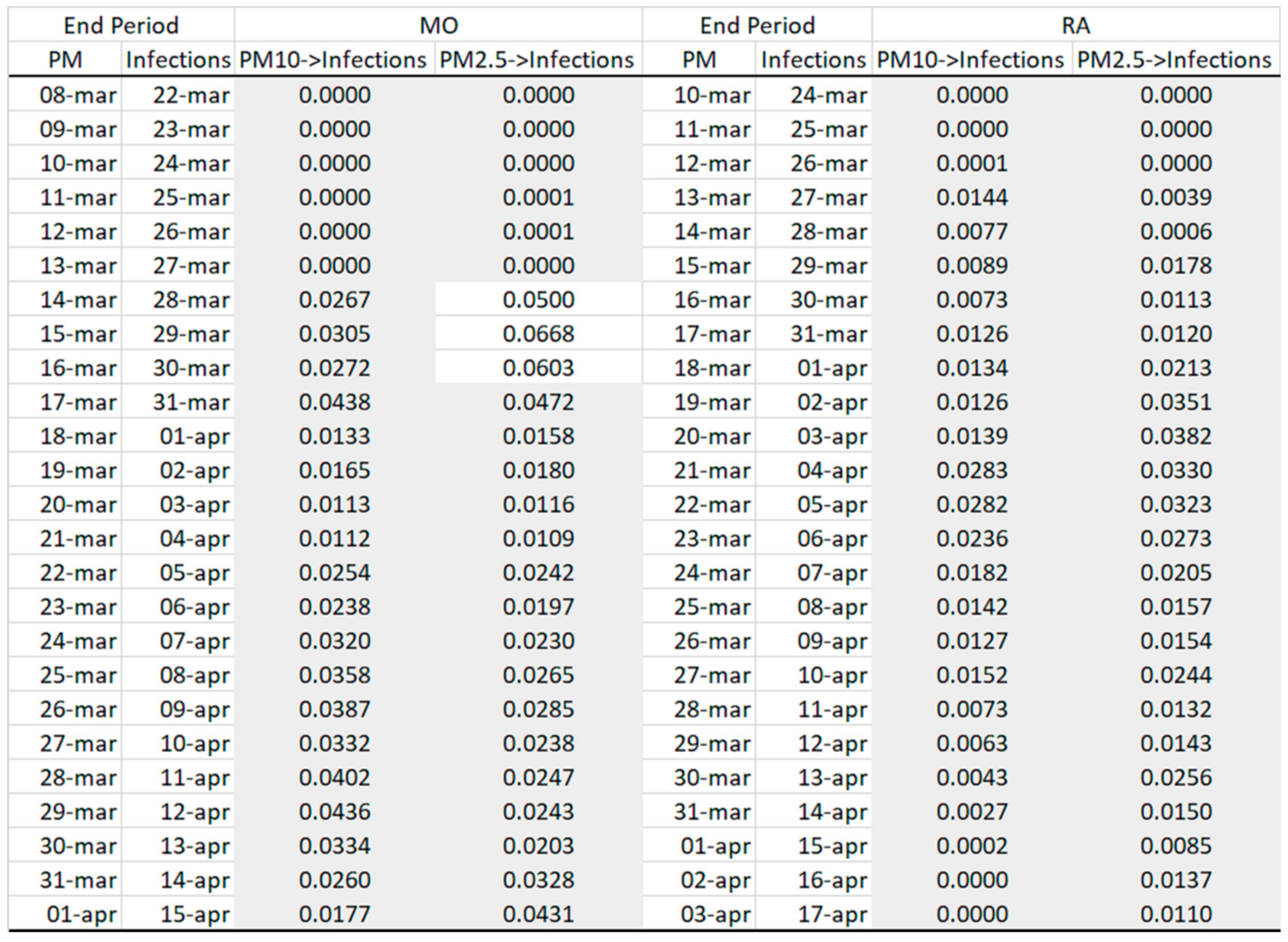
All this said, Figure 5 reports the results of our Granger causality analysis conducted for the provinces of both Modena (MO) and Ravenna (RA).
For a full comprehension of the Figure, one should notice that all has remained unchanged here, with respect to Figure 4, as to how the experiments were developed, with just these three natural considerations:
- Each observed series closes in a period ranging, respectively, from 8 March (Modena) and 10 March (Ravenna) for the pollutants’ series, and from 22 March (Modena) and from 24 March (Ravenna) for the infections, up to 1 April (Modena) and to 13 April (Ravenna) for the pollutants’ series, and up to 15 April (Modena) and to 17 April (Ravenna) for the infections;
- The beginning day for both series (pollution and infections) remains the same as in the comments provided for Figure 4.
- The analysis, this time, was conducted just for the particulate matter of type: PM2.5 and PM10, not being available at that time stable measurements for NO2.
In essence, our scientific target, here, was to verify if the pairwise series correlation observed before was still confirmed, even if we have been adding some more 25 days at each series, with all the 25 days happened after that the lockdown took place.
To this aim, an analysis of the p - values of Figure 5 shows that we have got a total amount of 97 (out of 100) statistical confirmations (yielding a 97% value) that X Granger causes Y; that is, that some given pollutants have some effect on the number of infections, from a Granger-causality perspective.
To be precise, interesting is the fact that a similar analysis conducted for all the other provinces (Bologna, Ferrara, Forlì-Cesena, Parma, Piacenza, Reggio nell’Emilia and Rimini) provides a more controversial result, with a lower number of statistical confirmations (approximately around 50%), probably depending on all those interferences, happened as a consequence of the lockdown, which we mentioned before as the motivation of our decision for the exclusion.
Nonetheless, at the end of this study, we can maintain that strong statistical clues emerge in favor of a causal correlation between pollution and infections, at least in Emilia-Romagna. This should be confirmed by those readers who are taking into serious consideration the fact that we have conducted a careful study, based on an analysis of time series, considered both before and after the lockdown, and aimed at screening off all the typical limitations that can afflict the Granger causality hypothesis testing method.
4. Conclusions
We have conducted a statistical analysis that confirms, under a Granger causality perspective, that a causal correlation may exist between the two researched phenomena of: pollution and COVID-19 infections, in Emilia-Romagna, Italy. Here, we survey, at the end of the paper, the possible limitations of our study (as well as, its potentials).
As to this issue of possible fallacies and limitations of our investigations, we feel necessary to discuss, at least, on the three following points: (i) the robustness of the scientific methodology we adopted, (ii) the choice of the Emilia-Romagna region as the primary subject of our study, and finally (iii) the scientific validity of the data we used.
As far as the Granger causality method is concerned, we have already admitted that neither Granger, nor any other statistical testing procedure, can provide a final evidence that the two phenomena we have studied (i.e., pollution vs. COVID-19 infections) are definitely correlated in nature. In fact, to achieve an ultimate knowledge of this correlation, statistical evidences, like those demonstrated in this paper, should be always accompanied by additional experiments at a scale that is appropriate to the observed phenomena; that is, in this case, at a biomedical, chemical or even physical level. Apart from this issue, our study has demonstrated that using Granger may be a valid solution, over alternative computational methodologies, to infer statistical evidences from sets of data subjected to high levels of temporal uncertainty [35]. In this case, in particular, fundamental has been the idea of testing the correlation hypothesis with data taken both before and after the lockdown.
To move on to the second issue, we understand very well that the choice to limit our study to the Italian region of Emilia-Romagna can be a source of controversy, and a limitation, as well. However, none should forget that the COVID-19 pandemic spread to Italy very early in 2020, and that the virus hit this nation with a number of active cases (i.e., infections), and deaths, that were unmatched in Europe, at least at that time of the year. It is also another truth that the region hit hardest in Italy was Lombardy (with almost the 48% of all the fatalities in Italy). Nonetheless, we all know very well that Lombardy is still Italy’s COVID-19 hotspot, probably due to a combination of factors, including wrong medical, governmental, and industrial policies which are controversial, yet not negligible [36].
The Emilia-Romagna region was severely devasted, too (with almost the 12% of all the fatalities in Italy). However, regardless the size of the investigated sample, the relative absence of dispute on external factors, like overwhelmed hospitals and controversial decision making, at both a political and an industrial level, made this specific region a subject of study where the phenomena of interest (that is, pollution and infections) could emerge without an annoying level of external interferences.
Finally, it is the turn of the data. First, we want to emphasize that all the used data and statistics were publicly available, at the time of our investigation, on Italian governmental sites, precisely [1,27,28]. It is also worth noticing that all our experiments are reproducible using the data available in the public repositories we have mentioned. Nevertheless, it is also a fact that COVID-19 infections are by now assumed to be more widespread than initially expected, thus making many of the studies conducted so far (including ours) a poor proxy for understanding the extension of this infection, with all the relative implications [37]. Anyway, as already mentioned at the beginning of this paper, if we move beyond the relevance of our results, towards the real extent of the correlation we have statistically demonstrated, our ultimate aim is that of reinvigorating the debate on a scientific case (pollution vs. COVID-19), that should not go unsolved or remain uninvestigated.
As a very final note, it is worth mentioning that, for the sake of completeness, we have provided a graphical summarization of all the data we have used on our study in the Appendix A that follows this paper.
Author Contributions
All authors contributed equally to the manuscript. All authors have read and agreed to the published version of the manuscript.
Funding
This research received no external funding.
Conflicts of Interest
The authors declare no conflict of interest.
Appendix A
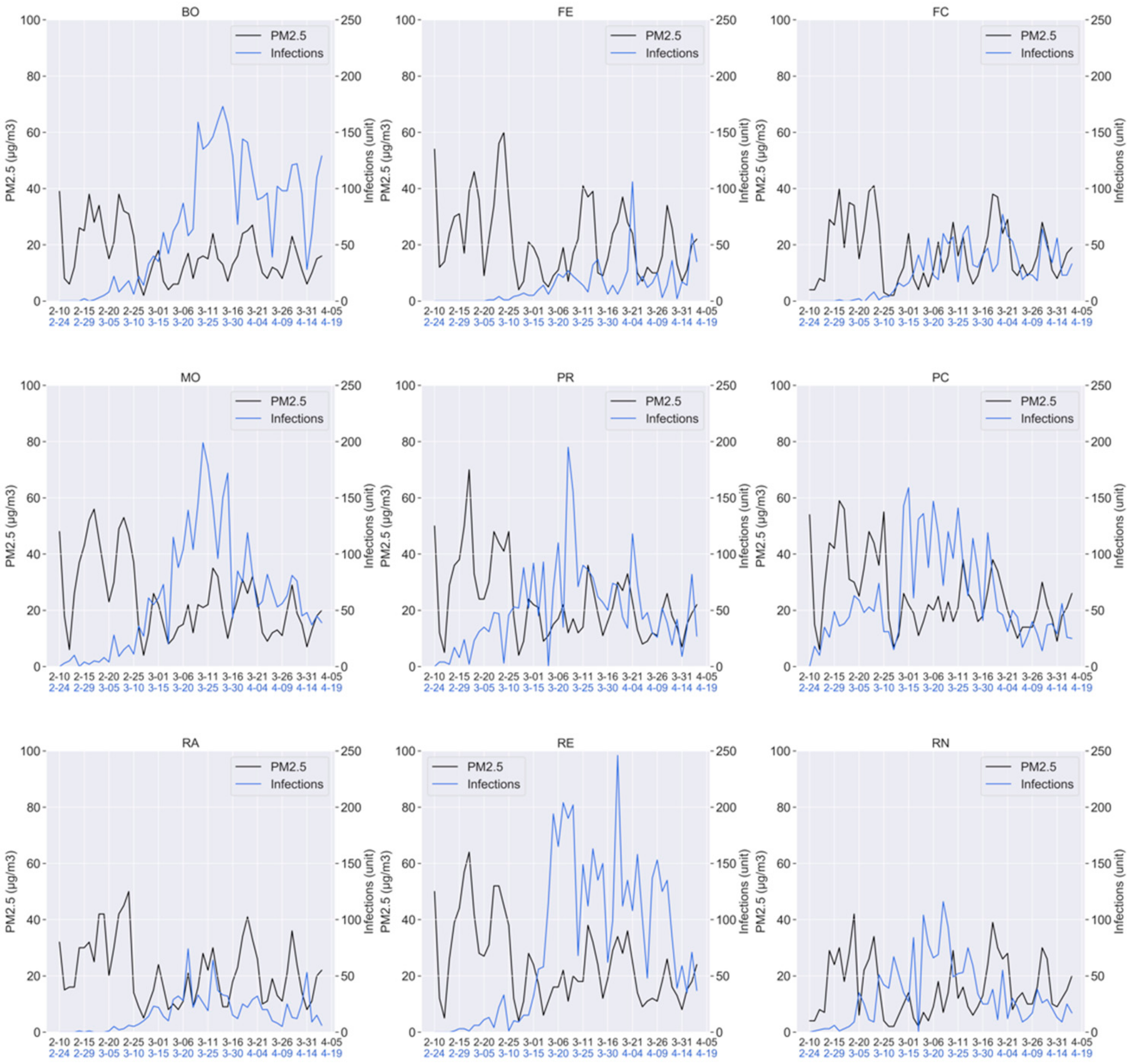
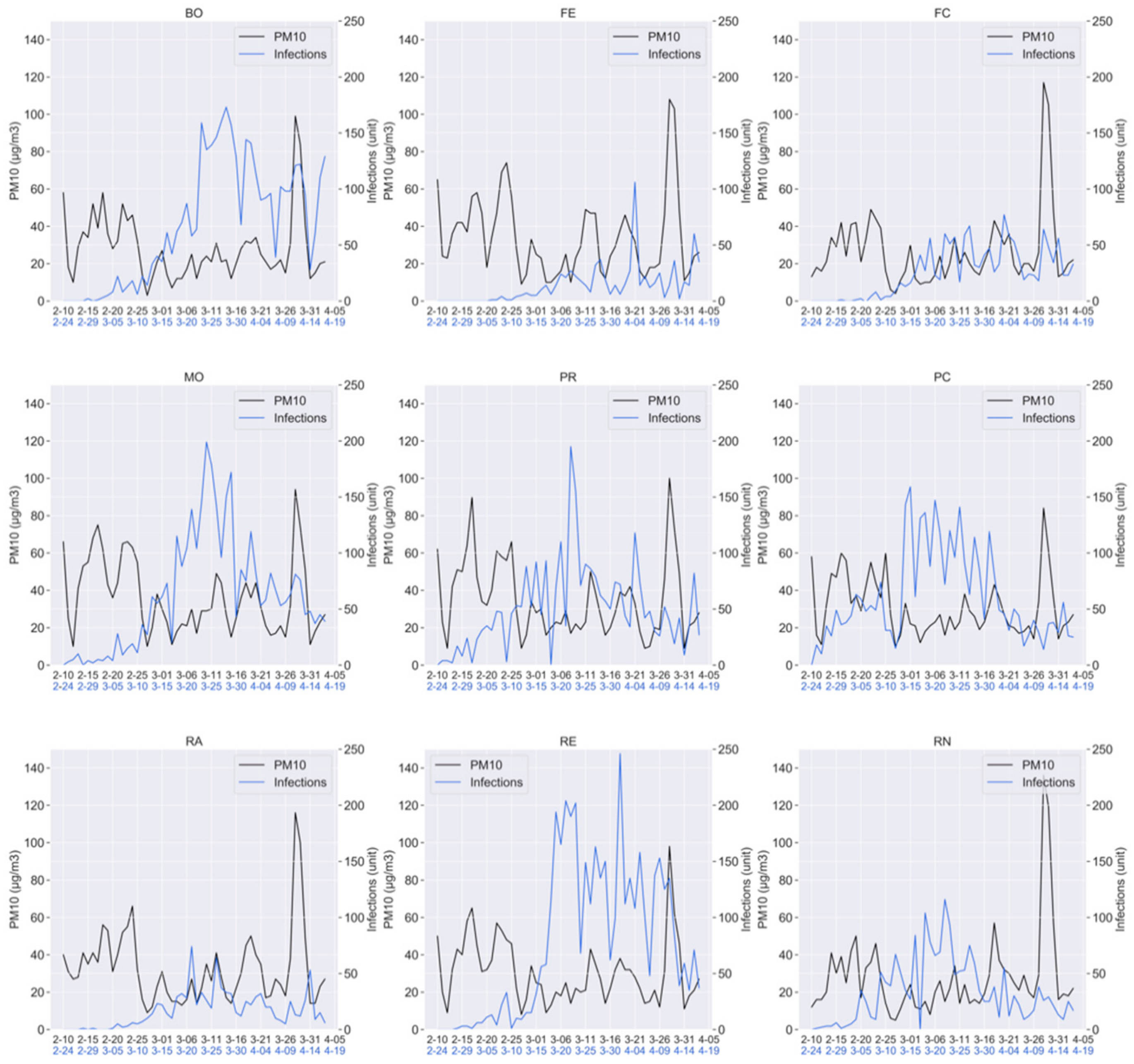
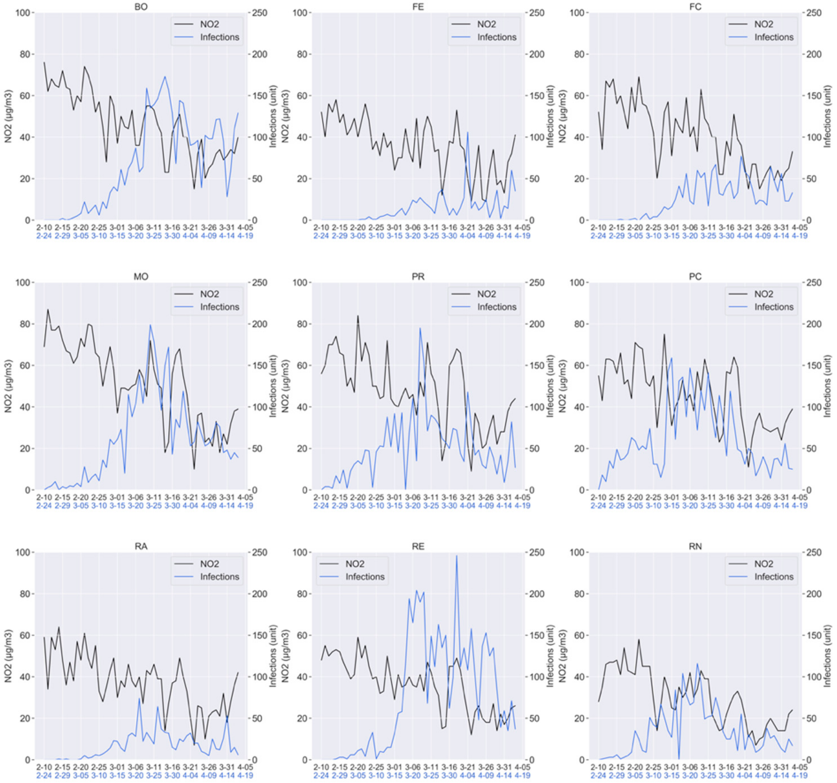
We provide a summarization of all the data we used for our experiments. These graphs simultaneously show the curves for both the pollutants (black) and the COVID-19 infections (blue). On the x axis of all graphs reported are the timelines for the pollutants’ series (in black) and for the infections (in blue). Figure A1, Figure A2 and Figure A3 are, respectively, concerned with: PM2.5, PM10 and NO2.
Figure A1.
Particulate matter (PM2.5) and COVID-19 infections (all the examined periods).

Figure A2.
Particulate matter (PM10) and COVID-19 infections (all the examined periods).

Figure A3.
Particulate matter (NO2) and COVID-19 infections (all the examined periods).

References
- Istituto Nazionale di Statistica. Impatto Dell’epidemia COVID-19 Sulla Mortallità Totale Della Popolazione Residente Primo Trimestre 2020. Available online: https://www.istat.it/en/files//2020/05/Rapporto_Istat_ISS.pdf (accessed on 6 May 2020).
- Jiang, Y.; Wu, X.J.; Guan, Y.J. Effect of ambient air pollutants and meteorological variables on COVID-19 incidence. Infect. Control Hosp. Epidemiol. 2020, 1–11. [Google Scholar] [CrossRef] [PubMed]
- You, S.; Tong, Y.W.; Neoh, K.G.; Dai, Y.; Wang, C.H. On the association between outdoor PM2.5 concentration and the seasonality of tuberculosis for Beijing and Hong Kong. Environ. Pollut. 2016, 218, 1170–1179. [Google Scholar] [CrossRef] [PubMed] [Green Version]
- Horne, B.D.; Joy, E.A.; Hofmann, M.G.; Gesteland, P.H.; Cannon, J.B.; Lefler, J.S.; Blagev, D.P.; Korgenski, E.K.; Torosyan, N.; Hansen, G.I.; et al. Short-term elevation of fine particulate matter air pollution and acute lower respiratory infection. Am. J. Respir. Crit. Care Med. 2018, 198, 759–766. [Google Scholar] [CrossRef] [PubMed]
- Su, W.; Wu, X.; Geng, X.; Zhao, X.; Liu, Q.; Liu, T. The short-term effects of air pollutants on influenza-like illness in Jinan, China. BMC Public Health 2019, 19, 1319. [Google Scholar] [CrossRef] [Green Version]
- Lee, G.I.; Saravia, J.; You, D.; Shrestha, B.; Jaligama, S.; Hebert, V.Y.; Dugas, T.R.; Cormier, S.A. Exposure to combustion generated environmentally persistent free radicals enhances severity of influenza virus infection. Part. Fibre Toxicol. 2014, 11, 57. [Google Scholar] [CrossRef] [Green Version]
- Carbone, M.; Green, J.B.; Bucci, E.M.; Lednicky, J.A. Coronaviruses: Facts, Myths, and Hypotheses. J. Thorac. Oncol. 2020, 15, 675–678. [Google Scholar] [CrossRef] [PubMed]
- Liang, Y.; Fang, L.; Pan, H.; Zhang, K.; Kan, H.; Brook, J.R.; Sun, Q. PM 2.5 in Beijing–temporal pattern and its association with influenza. Environ. Health 2014, 13, 102. [Google Scholar] [CrossRef] [Green Version]
- Feng, C.; Li, J.; Sun, W.; Zhang, Y.; Wang, Q. Impact of ambient fine particulate matter (PM 2.5) exposure on the risk of influenza-like-illness: A time-series analysis in Beijing, China. Environ. Health 2016, 15. [Google Scholar] [CrossRef] [Green Version]
- Li, Q.; Guan, X.; Wu, P.; Wang, X.; Zhou, L.; Tong, Y.; Ren, R.; Leung, K.S.M.; Lau, E.H.Y.; Wong, J.Y.; et al. Early transmission dynamics in Wuhan, China, of novel coronavirus–infected pneumonia. New Engl. J. Med. 2020, 382, 1199–1207. [Google Scholar] [CrossRef]
- Zhou, P.; Yang, X.L.; Wang, X.G.; Hu, B.; Zhang, L.; Zhang, W.; Si, H.R.; Zhu, Y.; Li, B.; Huang, C.L.; et al. A pneumonia outbreak associated with a new coronavirus of probable bat origin. Nature 2020, 579, 270–273. [Google Scholar] [CrossRef] [PubMed] [Green Version]
- Brankston, G.; Gitterman, L.; Hirji, Z.; Lemieux, C.; Gardam, M. Transmission of influenza A in human beings. Lancet Infect. Dis. 2007, 7, 257–265. [Google Scholar] [CrossRef]
- Tellier, R. Aerosol transmission of influenza A virus: A review of new studies. J. R. Soc. Interface 2009, 6, S783–S790. [Google Scholar] [CrossRef] [PubMed] [Green Version]
- Hinds, W.C. Properties, behavior, and measurement of airborne particles. In Aerosol Technology, 2nd ed.; John Wiley and Sons Press: New York, NY, USA, 1999; pp. 182–204. [Google Scholar]
- Nunez Soza, L.; Jordanova, P.; Nicolis, L.; Strelec, L.; Stehlik, M. Small sample robust approach to outliers and correlation of Atmospheric Pollution and Health Effects in Santiago de Chile. Chemom. Intell. Lab. Syst. 2019, 185, 73–84. [Google Scholar] [CrossRef]
- Pansini, R.; Fornacca, D. Initial evidence of higher morbidity and mortality due to SARS-CoV-2 in regions with lower air quality. MedRxiv Preprint 2020. [Google Scholar] [CrossRef]
- Wu, X.; Nethery, R.C.; Sabath, B.M.; Braun, D.; Dominici, F. Exposure to air pollution and COVID-19 mortality in the United States. 2020. Available online: https://www.medrxiv.org/content/10.1101/2020.04.05.20054502v2 (accessed on 25 April 2020).
- Ogen, Y. Assessing nitrogen dioxide (NO2) levels as a contributing factor to the coronavirus (COVID-19) fatality rate. Sci. Total Environ. 2020, 726, 138605. [Google Scholar] [CrossRef] [PubMed]
- Setti, L.; Passarini, F.; De Gennaro, G.; Baribieri, P.; Perrone, M.G.; Borelli, M.; Palmisani, J.; Di Gilio, A.; Torboli, V.; Pallavicini, A.; et al. SARS-Cov-2 RNA Found on Particulate Matter of Bergamo in Northern Italy: First Preliminary Evidence. Available online: https://www.medrxiv.org/content/10.1101/2020.04.15.20065995v2 (accessed on 2 May 2020).
- Setti, L.; Passarini, F.; De Gennaro, G.; Barbieri, P.; Perrone, M.G.; Piazzalunga, A.; Borelli, M.; Palmisani, J.; Di Giglio, A.; Piscitelli, P.; et al. The Potential role of Particulate Matter in the Spreading of COVID-19 in Northern Italy: First Evidence-based Research Hypotheses. 2020. Available online: https://www.medrxiv.org/content/10.1101/2020.04.11.20061713v1 (accessed on 25 April 2020).
- Conticini, E.; Frediani, B.; Caro, D. Can atmospheric pollution be considered a co-factor in extremely high level of SARS-CoV-2 lethality in Northern Italy? Environ. Pollut. 2020, 261, 114465. [Google Scholar] [CrossRef]
- Becchetti, L.; Conzo, G.; Conzo, P.; Salustri, F. Understanding the Heterogeneity of Adverse COVID-19 Outcomes: The Role of Poor Quality of Air and Lockdown Decisions. Available online: https://papers.ssrn.com/sol3/papers.cfm?abstract_id=3572548 (accessed on 25 April 2020).
- Caserini, S.; Perrino, C.; Forastiere, F.; Poli, G.; Vicenzi, E.; Carra, L. Pollution and COVID. Two Vague Clues don’t Make an Evidence. Available online: http://www.scienceonthenet.eu/articles/pollution-and-COVID-two-vague-clues-dont-make-evidence/stefano-caserini-cinzia-perrino (accessed on 29 April 2020).
- Maziarz, M. A review of the Granger-causality fallacy. J. Philos. Econ. 2015, 8, 86–105. [Google Scholar]
- Gazzetta Ufficiale della Repubblica Italiana. Decreto del Presidente del Consiglio dei Ministri 8 Marzo 2020. Available online: https://www.gazzettaufficiale.it/eli/id/2020/03/08/20A01522/sg (accessed on 20 April 2020).
- Governo Italiano Presidenza del Consiglio dei Ministri. Available online: http://www.governo.it/it/articolo/firmato-il-dpcm-9-marzo-2020/14276 (accessed on 20 April 2020).
- COVID-19 Italia—Monitoraggio Situazione. Available online: https://github.com/pcm-dpc/COVID-19 (accessed on 18 April 2020).
- Arpae Emilia-Romagna. Available online: https://arpae.it/mappa_qa.asp?idlivello=1682&tema=stazioni (accessed on 18 April 2020).
- Lauer, S.A.; Grantz, K.H.; Bi, Q.; Jones, F.K.; Zheng, Q.; Meredith, H.R.; Azman, A.S.; Reich, N.G.; Lessler, J. The incubation period of coronavirus disease 2019 (COVID-19) from publicly reported confirmed cases: Estimation and application. Ann. Intern. Med. 2020, 172, 577–582. [Google Scholar] [CrossRef] [Green Version]
- Cereda, D.; Tirani, M.; Rovida, F.; Demicheli, V.; Ajelli, M.; Poletti, P.; Trentini, F.; Guzzetta, G.; Marziano, V.; Barone, A.; et al. The early Phase of the COVID-19 Outbreak in Lombardy, Italy. Available online: https://arxiv.org/abs/2003.09320 (accessed on 25 April 2020).
- Granger, C. Investigating Causal Relations by Econometric Models and Cross-spectral Methods. Econometrica 1969, 37, 424–438. [Google Scholar] [CrossRef]
- Granger, C.W. Testing for causality: A personal viewpoint. J. Econ. Dyn. Control 1980, 2, 329–352. [Google Scholar] [CrossRef]
- Dickey, D.; Fuller, W. Distribution of the estimators for autoregressive time series with a unit root. J. Am. Stat. Assoc. 1979, 74, 427–431. [Google Scholar] [CrossRef]
- Arntzenius, F. The common cause principle. In 1992 Biennial Meeting of the Philosophy of Science Association; The University of Chicago Press: Chicago, IL, USA, 1992; Volume 2, pp. 227–237. [Google Scholar]
- Delnevo, G.; Roccetti, M.; Mirri, S. Modeling Patients’ Online Medical Conversations: A Granger Causality Approach. In Proceedings of the 2018 IEEE/ACM International Conference on Connected Health: Applications, Systems and Engineering Technologies, Washington, DC, USA, 26–28 September 2018; IEEE: Piscataway, NJ, USA, 2018; pp. 40–44. [Google Scholar] [CrossRef] [Green Version]
- Privitera, G. First in, Last Out: Why Lombardy is Still Italy’s Coronavirus Hotspot. Politico. 2020. Available online: https://www.politico.eu/article/first-in-last-out-why-lombardy-is-still-italys-coronavirus-COVID19-hotspot-italy/ (accessed on 13 June 2020).
- Sood, N.; Simon, P.; Ebner, P. Seroprevalence of SARS-CoV-2–Specific Antibodies Among Adults in Los Angeles County, California, on April 10–11, 2020. J. Am. Med Assoc. 2020, 323, 2425–2427. [Google Scholar] [CrossRef] [PubMed]
Figure 1.
Causality structure: (a) mutual interaction, (b) causal relation.

Figure 2.
The role of the lag factor in the Granger formula: (a) without lag, (b) with lag.

Figure 3.
Comparing temporal series: traditional methods (a); à la Granger methods (b).

Figure 4.
Particulate matter and COVID-19 infections (before lockdown): Granger-causality and p-values.
Figure 4.
Particulate matter and COVID-19 infections (before lockdown): Granger-causality and p-values.

Figure 5.
Particulate matter and COVID-19 infections (after lockdown): Granger-causality and p-values.
Figure 5.
Particulate matter and COVID-19 infections (after lockdown): Granger-causality and p-values.

© 2020 by the authors. Licensee MDPI, Basel, Switzerland. This article is an open access article distributed under the terms and conditions of the Creative Commons Attribution (CC BY) license (http://creativecommons.org/licenses/by/4.0/).
Share and Cite
MDPI and ACS Style
Delnevo, G.; Mirri, S.; Roccetti, M. Particulate Matter and COVID-19 Disease Diffusion in Emilia-Romagna (Italy). Already a Cold Case? Computation 2020, 8, 59. https://0-doi-org.brum.beds.ac.uk/10.3390/computation8020059
AMA Style
Delnevo G, Mirri S, Roccetti M. Particulate Matter and COVID-19 Disease Diffusion in Emilia-Romagna (Italy). Already a Cold Case? Computation. 2020; 8(2):59. https://0-doi-org.brum.beds.ac.uk/10.3390/computation8020059
Chicago/Turabian StyleDelnevo, Giovanni, Silvia Mirri, and Marco Roccetti. 2020. "Particulate Matter and COVID-19 Disease Diffusion in Emilia-Romagna (Italy). Already a Cold Case?" Computation 8, no. 2: 59. https://0-doi-org.brum.beds.ac.uk/10.3390/computation8020059
Note that from the first issue of 2016, this journal uses article numbers instead of page numbers. See further details here.