A Modification of Gradient Descent Method for Solving Coefficient Inverse Problem for Acoustics Equations

Abstract

We investigate the mathematical model of the 2D acoustic waves propagation in a heterogeneous domain. The hyperbolic first order system of partial differential equations is considered and solved by the Godunov method of the first order of approximation. This is a direct problem with appropriate initial and boundary conditions. We solve the coefficient inverse problem (IP) of recovering density. IP is reduced to an optimization problem, which is solved by the gradient descent method. The quality of the IP solution highly depends on the quantity of IP data and positions of receivers. We introduce a new approach for computing a gradient in the descent method in order to use as much IP data as possible on each iteration of descent.

1. Introduction

In this paper we consider the direct and inverse problem for the hyperbolic system of the two dimensional acoustic wave propagation. These problems are related to ultrasound tomography [1,2,3], aimed at the detection of inclusions in the soft human tissue, which is connected with the development of methods and instruments for early breast cancer detection. This field was studied intensively lately [4,5,6,7,8,9,10]. On the mathematical level, such problems are usually formulated in terms of an inverse problem, where some parameters of the medium are to be determined by using additional information [11,12,13,14,15]. Thus, an important issue is the construction of effective algorithms for solving the inverse problem, and, therefore, direct problem due to their tightly connected efficiency.

We use the hyperbolic first-order system to describe the propagation of the acoustic waves. On the one hand, this allows to propose a more realistic model from the physical point of view. On the other hand, we can apply an optimization approach for recovering coefficients of such system, like the density of the medium, the speed of the wave propagation or the absorption coefficient.

We consider the system of hyperbolic equations of the first order as the mathematical model of the acoustic tomograph, because these equations are obtained directly from the conservation laws of continuum mechanics. It allows us to control the preservation of the basic invariants during the solution of direct and inverse problems. This is important for solving unstable problems, as the conservation laws of the main invariants are the only criterion of the well-posedness of the solution. When we use the hyperbolic system to formulate the problem, we can ensure that the numerical solution is close to the physical solution of the process.

We apply the numerical algorithm for solving direct problems, based on the S. K. Godunov scheme [16,17]. The numerical methods, based on the Godunov approach, allows to find the balance between mathematical modelling of physical process and the effective numerical realization. The finite-difference method allows for solving a direct problem for the acoustic equation proposed in [18]. The main difficulties in the solution of direct problems, which is based on finite approximation, are that if the parameters of the medium are piece-wise smooth functions we have to add glueing conditions at the media interface to guarantee the physical solution. If the media interfaces are not simple, it is very hard to add these conditions. When we solve the inverse problem we do not know exactly the media interfaces and it is impossible realise these conditions.

Well-posedness of the direct problems for linear hyperbolic systems were investigated in [19,20]. In [21], regularity results for several hyperbolic equations were obtained.

The mixed problem for the linear symmetric hyperbolic systems with maximally non-negative and characteristic boundary conditions was studied in [22]. The existence of a unique solution was proved inside a suitable class of functions of weighted Sobolev type (with coefficients from $L^{\infty }$), which takes account of the loss of regularity in the normal direction to the characteristic boundary.

The mixed initial-boundary value problem for a linear hyperbolic system with a characteristic boundary of constant multiplicity was investigated in [23]. Authors assumed the problem to be “weakly” well-posed, in the sense that a unique $L_2$-solution exists, for sufficiently smooth data, and obeys an a priori energy estimate with a finite loss of conormal regularity. Under the assumption of the loss of one conormal derivative, the regularity of solutions was obtained, in the natural framework of weighted anisotropic Sobolev spaces, provided the data are sufficiently smooth.

The first-order hyperbolic systems on an interval with dynamic boundary conditions are considered in [24]. The well-posedness for linear systems was established using an abstract Friedrichs theorem. Due to the limited regularity of the coefficients, authors introduced the appropriate space of test functions for the weak formulation. It was shown that the weak solutions exhibit a hidden regularity at the boundary as well as at interior points.

Numerical methods, suitable for solving the coefficient inverse problems for hyperbolic systems and equations, are usually divided into direct ones and iterative ones. Direct methods are based on the Gelfand–Levitan–Krein approach [25,26,27,28,29,30] and boundary control method [31,32]. It was shown that the discrete coefficients inverse problems equations, which arise in the Gelfand–Levitan–Krein approach and boundary control method, coincide [33,34]. Iteration methods are gradients [35,36,37,38,39] and global-convergence [12,40,41,42,43]. Newton-type methods also can be applied to the coefficient inverse problems, but in comparison with gradient methods, where we solve on each iteration direct and adjoint problem, in Newton methods on each iteration it is necessary to solve direct and one linear inverse problems. Even in the two-dimensional case, solving a linear inverse problem is rather complicated.

Some considerations for choosing the model, based on the first-order system and the method for solving such system, can be found in [44,45].

In this work we use the gradient-based method to minimize the cost functional. However, such approach requires quite a significant amount of computations. Thus, in order to retain the acceptable performance of the method, one has to effectively use the available data.

Inverse problems for hyperbolic systems with data given on the part of the boundary were investigated in [46].

The standard gradient type method assumes that on each iteration the gradient is constructed via a solution of the direct and adjoint problem, which in its turn are obtained from fixed positions of source and receivers. In this article we present a new formula for the gradient type method where gradient constructs from direct and adjoint problem’s data obtained from different positions of sources and receivers in order to get more knowledge about unknown parameters of the medium.

The paper is organized as follows. In the first section we consider the main equations of the model, their connection to the conservation laws, and briefly describe the scheme of S.K. Godunov that we use for the numerical solution of the direct problem. The second section is dedicated to the inverse problem of recovering the density by using the pressure registered in the receivers. We consider the adjoint problem and the gradient of the cost functional that can be calculated using the solution of the direct and adjoint problems. In Section 4, we consider different approaches for using the additional sets of data, corresponding to the different locations of the source. The numerical comparative analysis of these approaches is considered in Section 5 in the case of exact and noised data. In the discussion, we consider the results obtained and the future work for developing the methods.

2. Direct Problem

2.1. Governing Equations

First we consider the direct problem of acoustic wave propagation through the 2D medium. We consider the following first order system of hyperbolic equations:

$$\begin{array}{c}\frac{\partial u}{\partial t}+\frac{1}{\rho }\frac{\partial p}{\partial x}=0,\frac{\partial v}{\partial t}+\frac{1}{\rho }\frac{\partial p}{\partial y}=0,(x,y)\in \mathsf{\Omega },0<t\le T,\end{array}$$

(1)

$$\begin{array}{c}\frac{\partial p}{\partial t}+\rho c^2\left(\frac{\partial u}{\partial x}+\frac{\partial v}{\partial y}\right)={\theta }_{\mathsf{\Omega }}(x,y)I\left(t\right),(x,y)\in \mathsf{\Omega },\end{array}$$

(2)

$$\begin{array}{c}{u,v,p|}_{(x,y)\in \partial \mathsf{\Omega }}=0,\end{array}$$

(3)

$$\begin{array}{c}{u,v,p|}_{t=0}=0.\end{array}$$

(4)

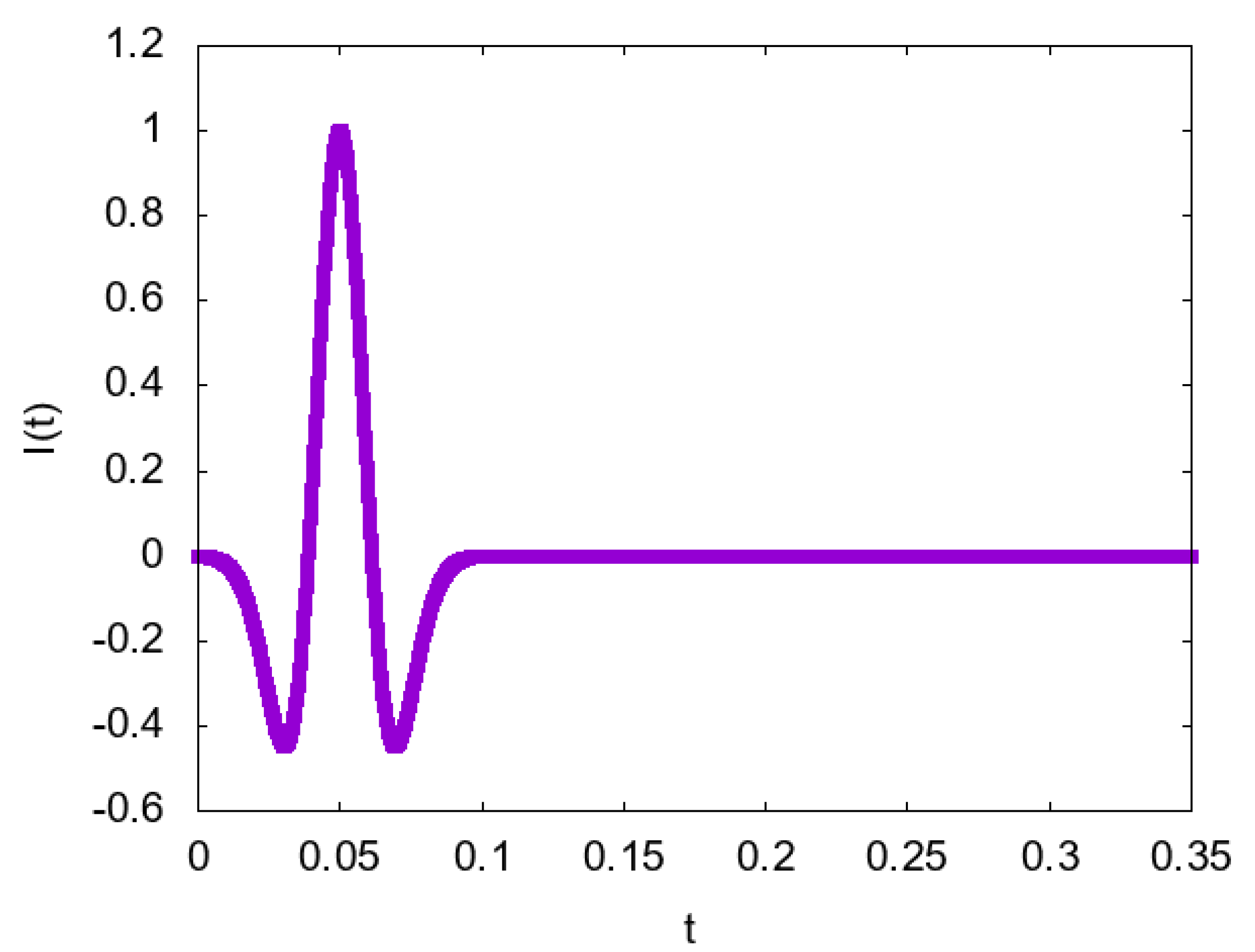
Here $u=u(x,y,t)$, $v=v(x,y,t)$ are components of the velocity vector, with respect to x and y respectively, $p=p(x,y,t)$ is the acoustic pressure. The parameters of the system describes the properties of the medium: $\rho (x,y)$ denotes the density of the medium, and $c(x,y)$ is the speed of the wave propagation. $\mathsf{\Omega }=(x,y)\in [0,L]\times [0,L]$, function ${\theta }_{\mathsf{\Omega }}$ describes the location of the source, $I\left(t\right)$ has the form of Ricker wavelet (Figure 1), where ${\nu }_0$ is a frequency:

$$I\left(t\right)=\left(1-2{\left(\pi {\nu }_0\left(t-\frac{1}{{\nu }_0}\right)\right)}^2\right)e^{-\pi {\nu }_0\left(t-\frac{1}{{\nu }_0}\right)}.$$

(5)

Equations (1) and (2) are tightly connected with the following integral equalities:

$$\begin{array}{c}\hfill \oint \rho udxdy+pdydt=0,\end{array}$$

(6)

$$\begin{array}{c}\hfill \oint \rho vdxdy+pdxdt=0,\end{array}$$

(7)

$$\begin{array}{c}\hfill \oint pdxdy+\rho c^2\left(udydt+vdxdt\right)=0.\end{array}$$

(8)

Equations (6) and (7) represent the conservation laws of impulse in direction x and y, while Equation (8) is the conservation law of mass. The connection between differential and integral formulations based on the fact that, on the one hand, one can integrate Equations (1) and (2) in an arbitrary domain to obtain Equations (6)–(8), and on the other hand, the continuum mechanics equations are usually derived in terms of integral conservation laws, and only after that it turns to differential equations.

2.2. Brief Introduction to Godunov Finite-Difference Scheme

We use the connection between Equations (1) and (2) and Equations (6)–(8) when solving direct problem Equations (1)–(4), as we consider the numerical method, proposed by S.K. Godunov in [17]. Its steps are introducing a numerical grid, considering Equations (6)–(8) in each numerical cell and moving from integral to finite-differences. The main element of this method is the solving of the Riemann problem (see below), which consists of an initial value problem composed of a conservation equation together with piece-wise constant data having a single discontinuity.

Let us consider numerical cell $(i-1/2,j-1/2)$ with boundaries $[i-1,j-1/2],[i,j-1/2]$ in dimension x, and $[j-1,i-1/2],[j,i-1/2]$ in dimension y, for $i\in 0\dots N_x-1,i\in 0\dots N_y-1$, where $N_x$ and $N_y$ are the number of grid points in each dimension. Then, the first of Equation (6) can be approximated via

$$(\rho u^{i-1/2,j-1/2}-\rho u_{i-1/2,j-1/2})h_x{h}_y+\tau h_y(P_{i,j-1/2}-P_{i-1,j-1/2})=0,$$

(9)

where for values in the cell sub-indexes indicate current time step, and sup-indexes—the next time step, $h_x,h_y$—grid steps in direction x and y, $\tau$—grid steps in time direction, and $P_{i,j-1/2}$—solution of additional problem at the boundary $(i,j-1/2)$, called the discontinuity decay problem or Riemann problem. In the same way two more approximated equations for Equations (7) and (8) can be derived. Solution of the discontinuity decay problem $P_{i,j-1/2}$ can be obtained by the following formula using values of pressure and velocity from adjacent to the boundary numerical cells:

$$p=P_{i,j-1/2}=\frac{p_{i-1/2,j-1/2}+p_{i+1/2,j-1/2}}{2}-{\rho }_0{c}_0\frac{u_{i+1/2,j-1/2}+u_{i-1/2,j-1/2}}{2}.$$

(10)

Constants ${\rho }_0,c_0$, for example, can be chosen as an average of values of density and sound speed from adjacent cells. One can find a full description of the Godunov method for the system of acoustic equations in [17].

3. Inverse Problem of Recovering the Density

Now we consider the inverse problem for the acoustic Equations (1)–(4). The data of the inverse problem is the pressure, registered in the receivers:

$$p(x_i,y_i,t)=f_i\left(t\right),i=1,\dots ,N.$$

(11)

In this paper we consider the inverse problem for recovering the density $\rho (x,y)$, using the data from Equation (11). The speed of sound $c(x,y)$ is a known function. We consider the cost functional:

$$J\left(\rho \right)={\int }_0^T\sum _{i=1}^N{\left[p(x_i,y_i,t;\rho )-f_i\left(t\right)\right]}^{2}dt\to \underset{\rho }{min}$$

(12)

Let us apply the gradient method for minimizing the cost functional

$${\rho }^{n+1}(x,y)={\rho }^n(x,y)-\alpha J^{\prime }\left({\rho }^n\right)(x,y).$$

(13)

Here $\alpha$ is a descent step, $J^{\prime }$ is a gradient of the functional J. Convergence of the iteration process for the coefficients inverse problems for hyperbolic equations were investigated in [37]. Using a priori information about the inverse problem solution in the algorithm was proposed in [47]. Gradient of cost functional can be calculated as follows [44]:

$$J^{\prime }\left(\rho \right)(x,y)={\int }_0^T\left[-{{\mathsf{\Psi }}_1}_{t}u-{{\mathsf{\Psi }}_2}_{t}v+\frac{1}{\rho }{\mathsf{\Psi }}_3(u_x+v_y)\right]dt.$$

(14)

Here, new functions ${\mathsf{\Psi }}_i,i=1,2,3$ solve the following adjoint problem [36,47]:

$$\begin{array}{c}{{\mathsf{\Psi }}_1}_t+\frac{1}{\rho }{{\mathsf{\Psi }}_3}_x=0;\end{array}$$

(15)

$$\begin{array}{c}{{\mathsf{\Psi }}_2}_t+\frac{1}{\rho }{{\mathsf{\Psi }}_3}_y=0;\end{array}$$

(16)

$$\begin{array}{c}\frac{1}{\rho c^2}{{\mathsf{\Psi }}_3}_t+({{\mathsf{\Psi }}_1}_x+{{\mathsf{\Psi }}_2}_y)=2\sum _{j=1}^N\delta (x-x_j,y-y_j)\left[p(x,y,t)-f_j\left(t\right)\right];\end{array}$$

(17)

$$\begin{array}{c}{\mathsf{\Psi }}_i(x,y,T)=0,i=1,2,3;\end{array}$$

(18)

$$\begin{array}{c}{\mathsf{\Psi }}_i{|}_{(x,y)\in \partial \mathsf{\Omega }}=0,i=1,2,3.\end{array}$$

(19)

Here, $\delta (x,y)$ is a Dirac delta-function. More details regarding the derivation of the adjoint problem and the gradient of the cost functional can be found in [35]. Therefore, each step of gradient descent requires the solution of direct problems in Equations (1)–(4), calculation of the residual and solution of the adjoint problem in Equations (15)–(19). Then we use the obtained solution of both the direct and adjoint problem to calculate the gradient $J^{\prime }\left(\rho \right)$ using Equation (14). Since the problem Equations (15)–(19) have the form of a first order system of hyperbolic equations, we apply the already mentioned Godunov scheme for solving Equations (15)–(19) during numerical experiments.

4. Modification of Gradient Descent Method

Let us consider a standard formula for the gradient descent method in Equation (13)

$${\rho }^{n+1}(x,y)={\rho }^{n+1}(x,y)-\alpha J^{\prime }\left({\rho }^{n+1}\right)(x,y).$$

In this way, on each iteration step we need to solve a direct problem, adjoint problem, and compute a gradient via the formula in Equation (14). Such way assumes that during optimization only the information from one source is used, because a system of source and receivers (inverse problem (IP) data) is fixed during one descent step. From a physical point of view, there is an influence of acoustic waves on the considered object only from a specific side. However, the data, obtained by the scattered waves from the single source is not enough to ensure the desired accuracy and efficiency of the method. Therefore, we have decided to rework the optimization approach in the following way to get more information. The idea is to use several different sources. Thus, we consider the new residual functional

$$J\left(\rho \right)=\sum _{i=1}^{N}J(\rho ;s_i).$$

(20)

where $J(\rho ;s_i)$ has the form of Equation (12) and corresponds to the source of acoustic waves, located in the point $s_i$. We suppose that we have the data corresponding to each source. The strategy of usage of such data could be different. Currently, the popular schemes are stochastic gradient descent (in our case this means the selection of the current number of the source $s_i$ in the random manner and then the update of the desired parameters, using the gradient of $J(\rho ;s_i)$) and the batch gradient descent (update the current approximation of the parameters using the gradients, corresponding to all sources, simultaneously) [48]. We use the latter approach, due to its computational efficiency and more stable convergence. However, the more detailed comparative analysis of the stochastic approach, batch descent and its mini-batch version, is the plan for future work and will be carried out later.

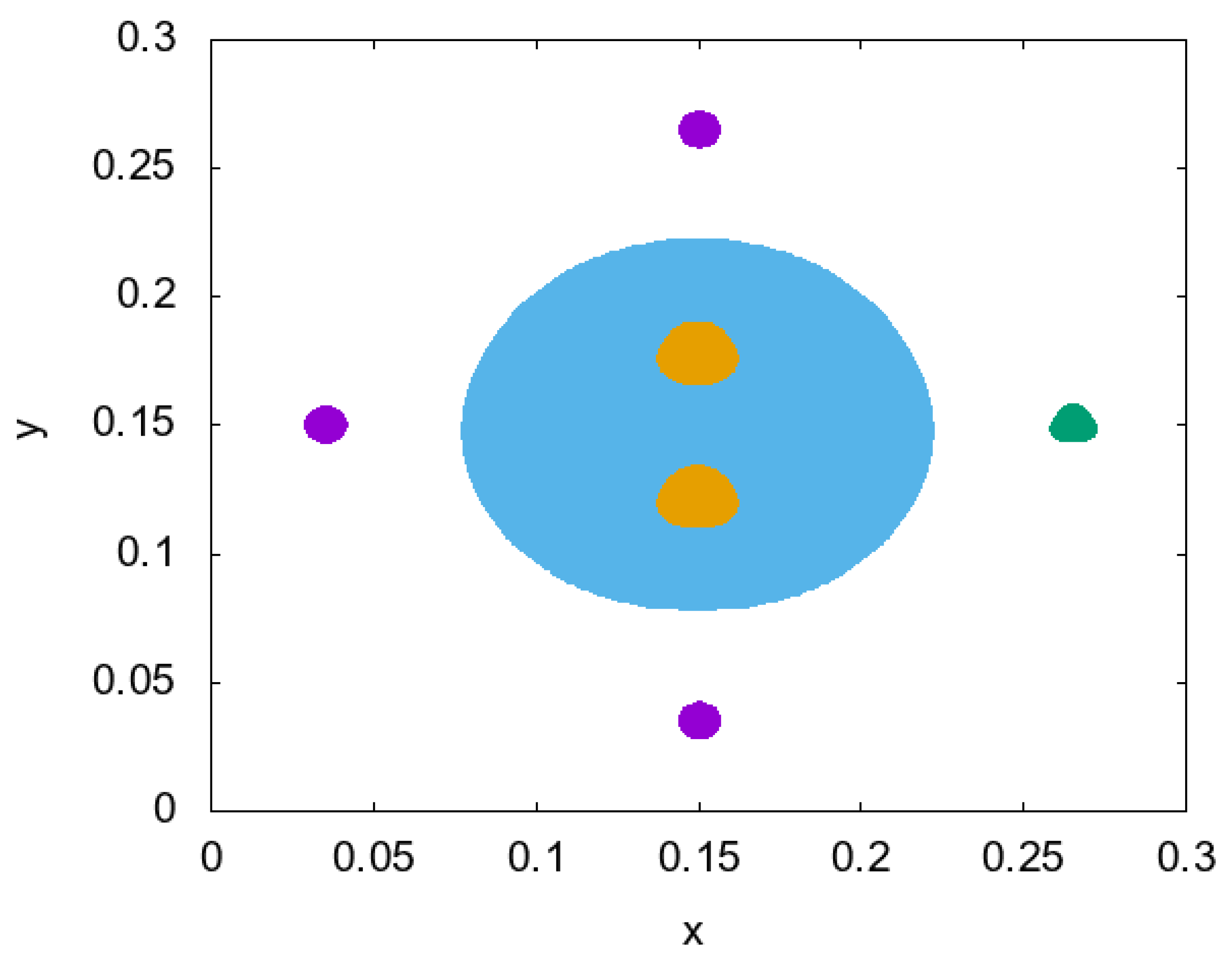
Let us denote the $J^{\prime }(\rho ;s_1)$ gradient that has been computed by solving direct and adjoint problems from the source in position $s_1$ and N−1 receivers, which represent a circle (see Figure 2).

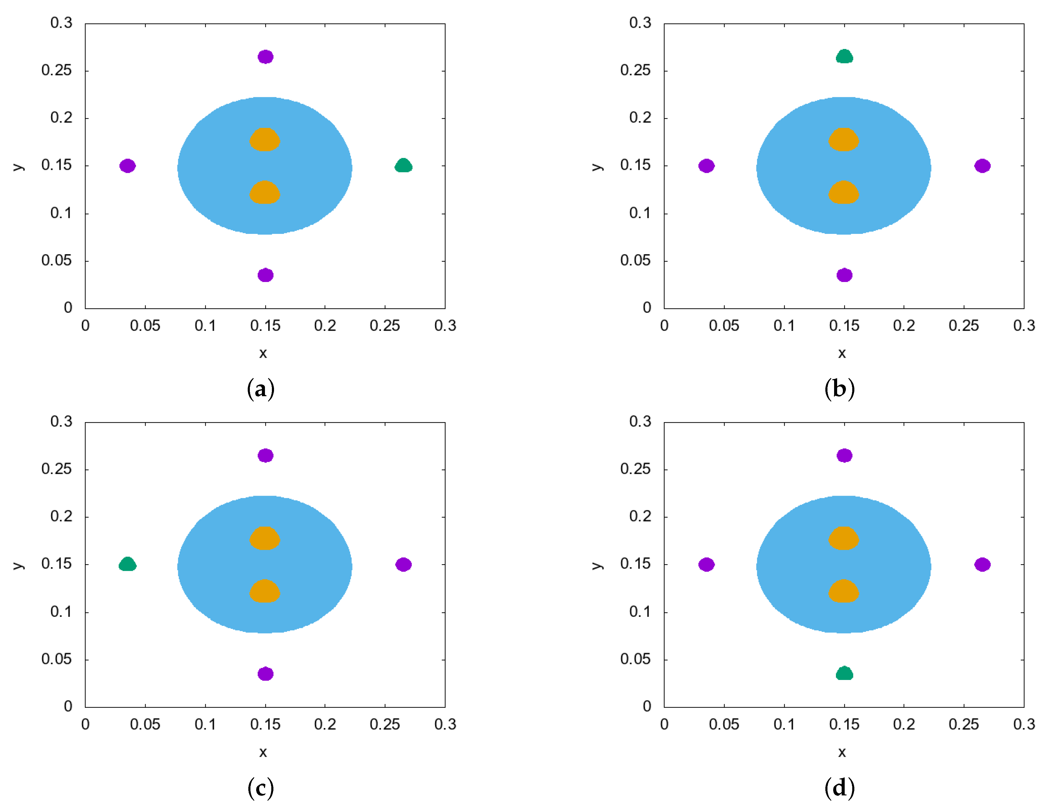
During one descent step let us change the position of source N—1 times as presented on Figure 3, for simplicity N = 4. In this example, position $s_1$ of the source has a 0 degree angle, $s_2$ is a 90 degree angle, $s_3$ is an 180 degree angle, and position $s_4$ a −270 degree angle (in centralized cartesian coordinates system). The blue colour represents the considered object, with unknown density in terms of the inverse problem. Two yellow points represent the inclusions inside the object. Our aim of solving the inverse problem is to reconstruct these inclusions with acceptable accuracy by using the optimization approach in Equation (12). We should mention that this model is used here only for illustration and simplicity—the models that were used during numerical experiments are presented in the next section.

In this way, on one iteration step we will get the data of N different direct and adjoint problems and compute N gradients $J^{\prime }(\rho ;s_i),i=1\dots N$. Of course, we can solve the N problems independently of each other and the parallelization of the algorithm can be the subject for future work. Then we construct a gradient descent method as follows:

$${\rho }^{n+1}={\rho }^n-\alpha \sum _{i=1}^N{J}^{\prime }({\rho }^n;s_i).$$

(21)

This new approach provides us information from different angles of view as “from source to object”. Unfortunately, this method is highly time-consuming, because one iteration of descent assumes solving of N direct and adjoint problems. However, numerical experiments show us that acceptable solutions can be obtained even for a few number of sources and receivers.

5. Numerical Results

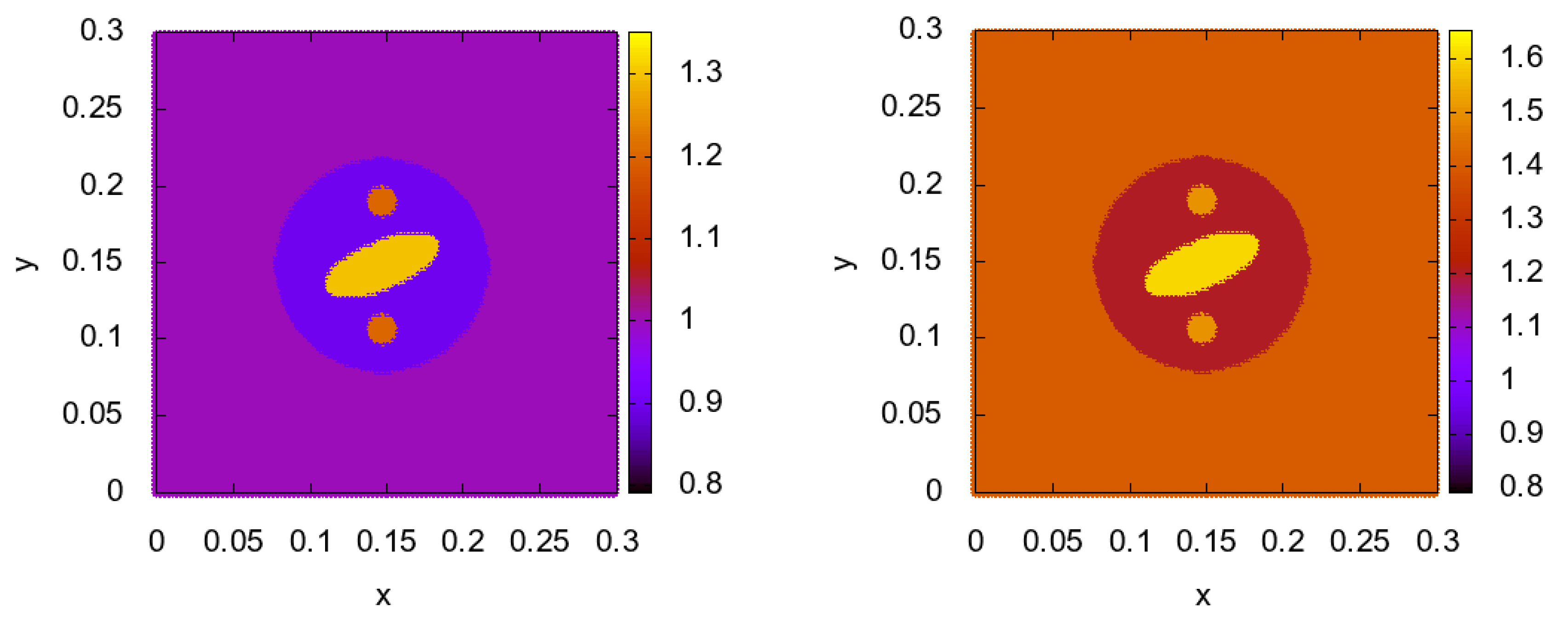
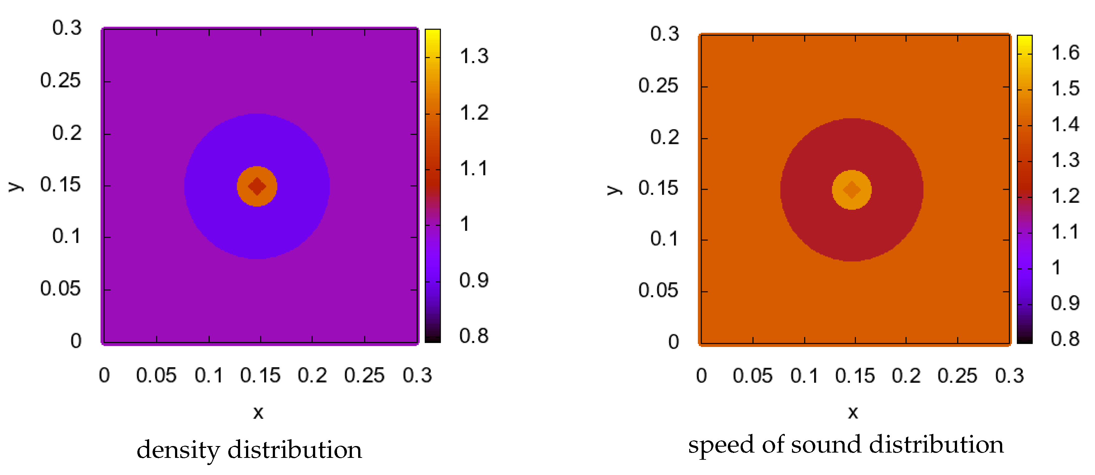
In this section we present numerical results of the inverse problem of density reconstruction. We consider the following artificial model, which consists of the test object, modelled as a circle, several inclusions inside the object, and the outer zone between the object and the transducers, filled with water. The parameters of the object are equal to normal human tissue ($\rho =0.9$ kg/m³, $c=1.2$ km/s), while the inclusions have higher density and speed of sound values (density is equal to $\rho =1.2$ kg/m³ in smaller inclusions and $\rho =1.3$ kg/m³ in larger ones, speed of sound is equal to $c=1.5$ km/s and $c=1.6$ km/s correspondingly). The exact structure of the model is presented in Figure 4. The size of inclusions was chosen according to the actual sizes of tumours at the first and second stages of breast cancer genesis. The physical size of computational domain is $[0,0.3]\times [0,0.3]$ meters. The numerical grid consists of $100\times 100$ points, and the CFL number was taken equal to 0.5 during the computations. We considered the synthetic data of inverse problems during the tests.

During numerical experiments we considered three variations of the gradient descent:

• Gradient constructed of 1 source, fixed in position $s_1$ (Figure 2). The formula of gradient descent is

  $${\rho }^{n+1}={\rho }^n-\alpha J^{\prime }({\rho }^n;s1).$$
• Gradient constructed of 1 source, but its location was changed on each iteration through positions $s_1,\dots ,s_{16}$, that are located uniformly on the circle of the radius $R=0.115$ m. The formula is in the next view

  $${\rho }^{n+1}={\rho }^n-\alpha J^{\prime }({\rho }^n;s_{[n/16]})$$
• Gradient constructed of 16 sources from positions $s_1,\dots ,s_{16}$ with each iteration in a cyclic manner. The final formula is

  $${\rho }^{n+1}={\rho }^n-\alpha \sum _{i=1}^N{J}^{\prime }({\rho }^n;s_i).$$

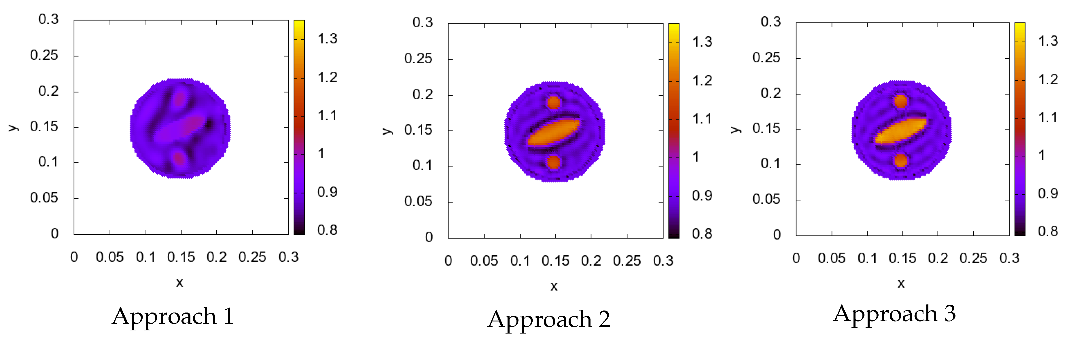
During the first experiment we compared these approaches after $N=1000$ iterations of descent. The results are presented in Figure 5.

All three inclusions could be seen. However, the accuracy of the density values differs for the approaches considered. The poor accuracy of the approach 1 is understandable—in this case much less data were obtained (one source in Approach 1 against 16 sources in Approaches 2 and 3). However, we have to compare Approaches 2 and 3 in order to understand how to better use the data obtained. One can find more detailed results in

Table 1. Relative errors and elapsed CPU time.

	Approach 1	Approach 2	Approach 3
Relative error	0.121	0.050	0.039
Elapsed time	40 s	40 s	480 s

below, where the relative error and computation time are presented.

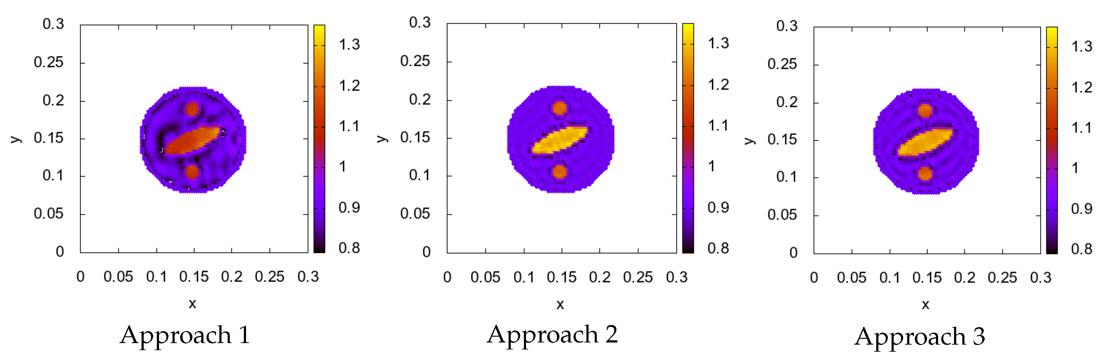
Despite the fact that the accuracy of Approach 3 is better, we pay for it with a large amount of computation time, since each iteration requires the solution of multiple direct problems (DP) and AP. In order to test the efficiency of the methods we have to equalize them in terms of CPU time. In our next test we considered 2000 iterations for Approach 3 and 16,000 iterations of Approaches 1 and 2. The results are presented by Figure 6 and

Table 2. Relative errors and elapsed CPU time.

	Approach 1	Approach 2	Approach 3
Relative error	0.071	0.026	0.032
Elapsed time	15 min	15 min	17 min

.

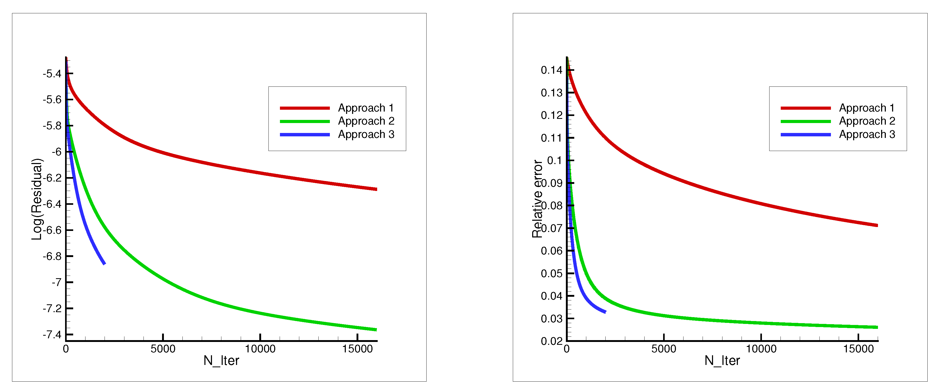
This case shows that the cyclic sweep through the sources is the better strategy. The third approach, based on a usage of multiple sources per one iteration provides faster decrease of residuals and errors of the method, but each iteration takes too much time, as shown in Figure 7.

We also tested the stability of the method. We added the noise to the data of the inverse problem in each receiver as follows:

$$\tilde{f}\left(t\right)=f\left(t\right)+\epsilon (f_{max}-f_{min})\gamma \left(t\right).$$

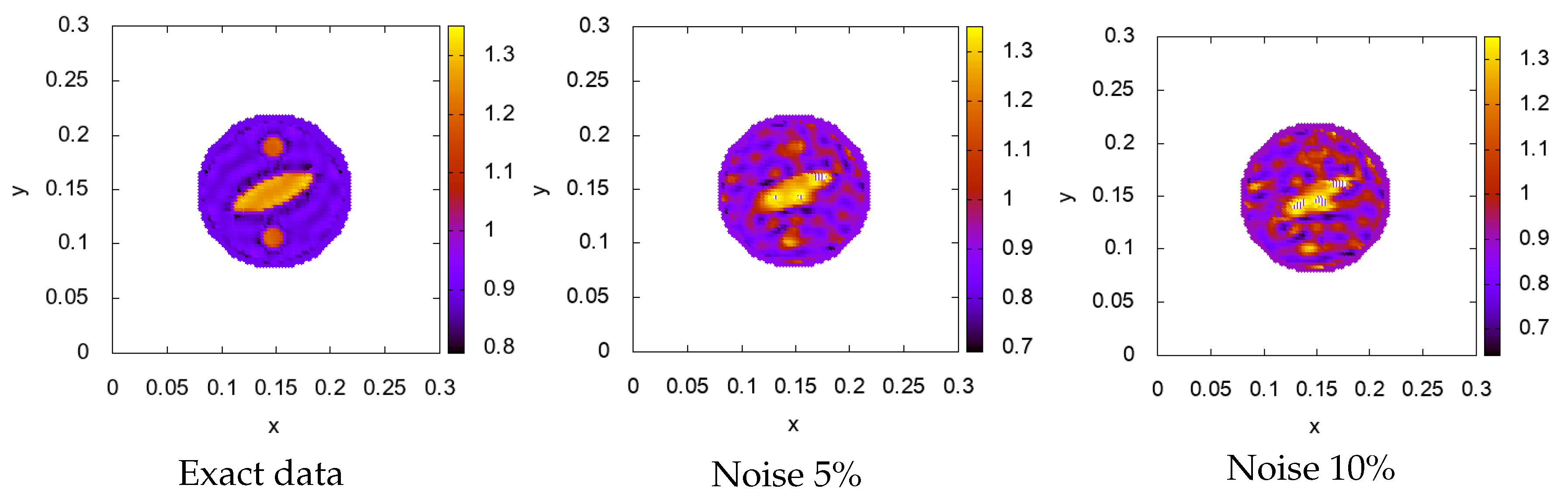
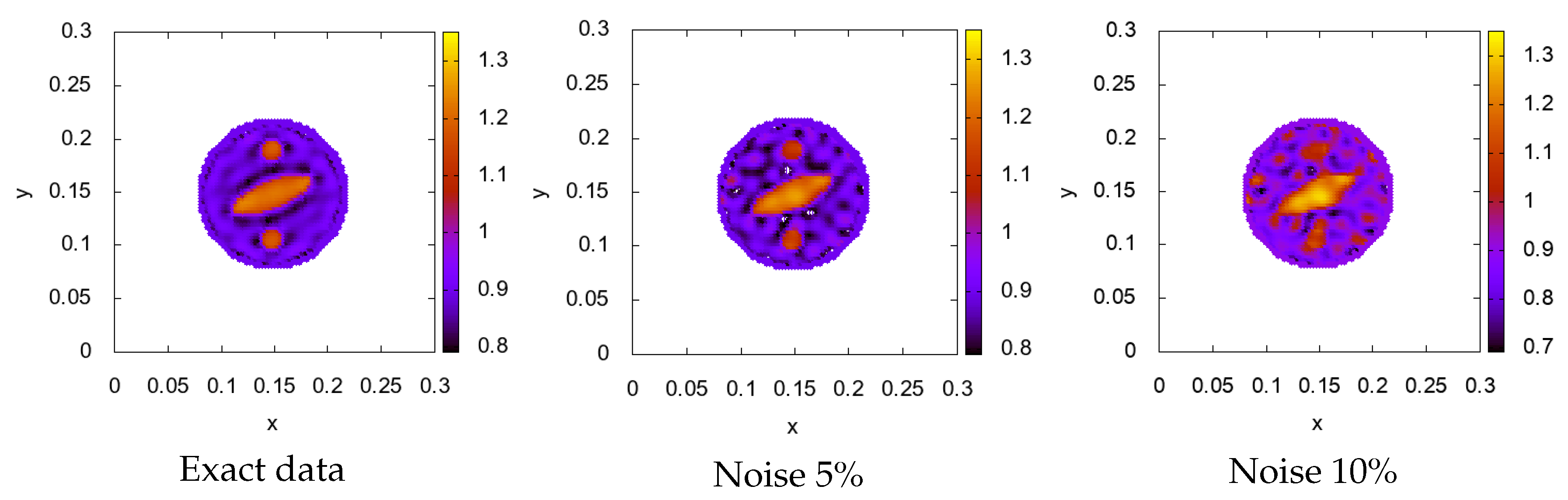
Here, $f\left(t\right)$ is the exact data, $\epsilon$ is the level of errors, $f_{max},f_{min}$—maximal and minimal values of the data, $\gamma \left(t\right)$—random variable, uniformly distributed on the interval $(-1,1)$. We also changed the number of sources/receivers to eight. As in the previous test, we considered 16,000 iterations for Approach 2 and 2000 iterations for Approach 3. The results are presented in Figure 8 and Figure 9.

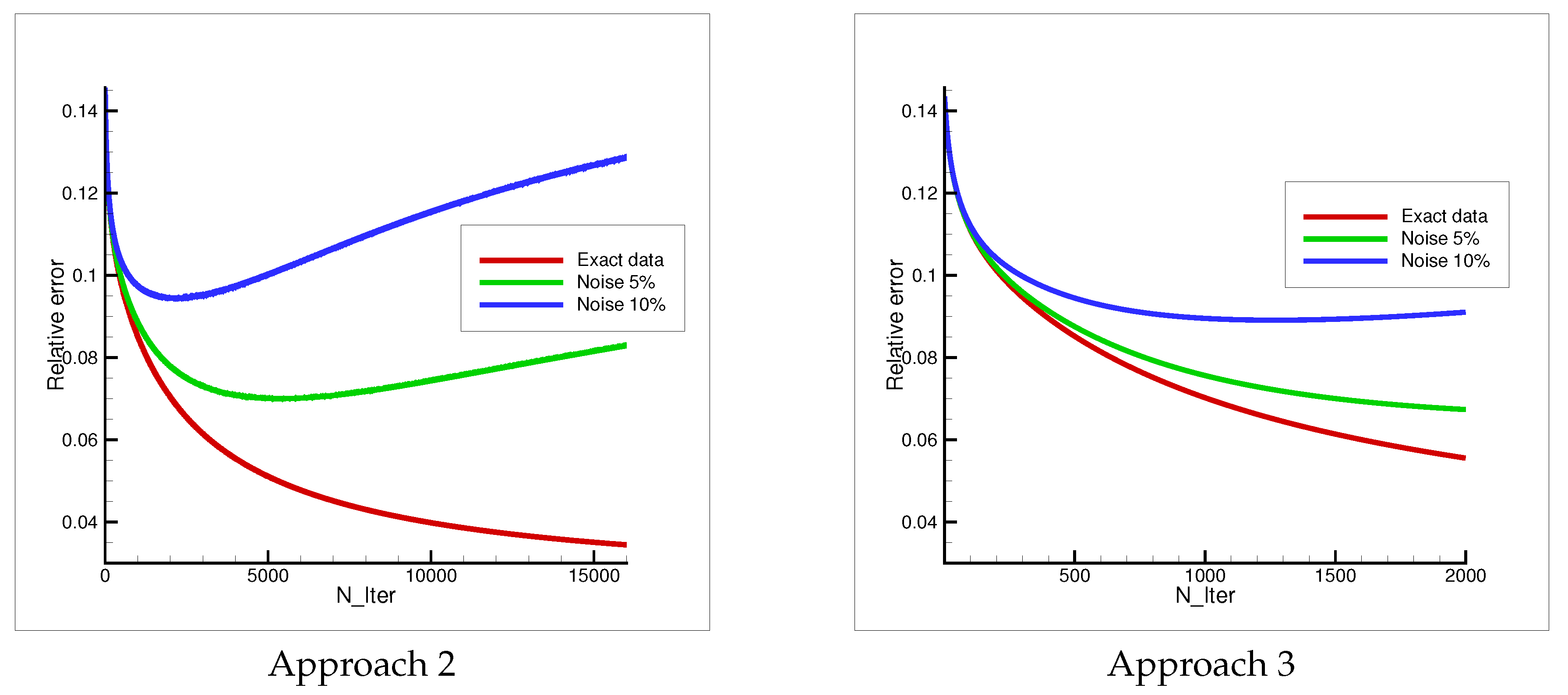
One can see that the usage of information from all sources on each iteration provides more stable results. In order to illustrate this behaviour, we consider Figure 10, where we consider the dependence of relative error on the iteration number for exact and noised data. One can see that in the case of Approach 2 and noised data, the error decreases only for the certain number of iterations and then starts to increase. The same holds for Approach 3 and the 10% noise level. Such situation is not rare for inverse and ill-posed problems and leads us to the fact that the iteration number should be considered as the regularization parameter [49,50,51]. We plan to address the question of the optimal number of iterations depending on the noise level in further work.

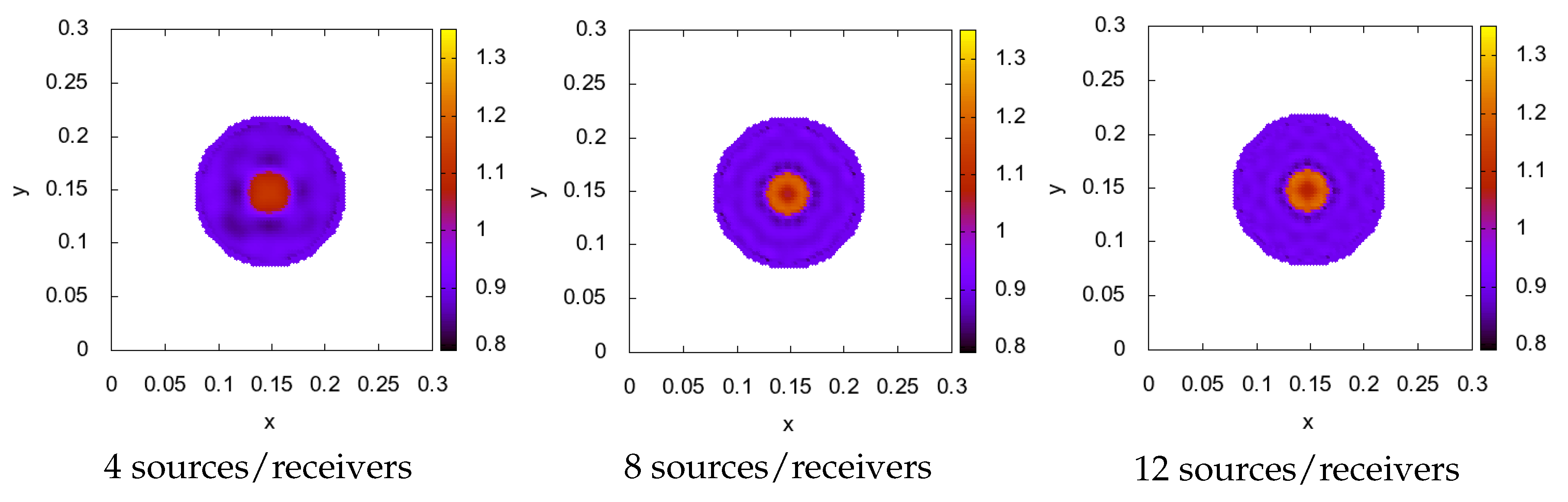
We also considered an additional test to check the resolution ability of the method. We considered the model, which contains one inclusion, similar to previous one, and another one, smaller and less densed, which is located inside the large inclusion. The exact structure of the model is presented in Figure 11.

In Figure 12 one can see the numerical results for a different number of sources/receivers. Here, we used Approach 2 (cyclic change of the source location), and the total iteration number was equal to 16,000. We will skip the results related to the usage of Approach 3. However, the behaviour of the methods is the same, as in the previous test—cyclic usage of the sources is more efficient in the case of the exact data, but the usage of multiple sources per iteration provides better results in the case of the noised data.

6. Discussion

We have considered the mathematical model of acoustic tomography, based on the system of hyperbolic equations of the first order. We have solved the coefficient inverse problem of density reconstruction for synthetic data. We proposed a new approach for constructing a gradient in the gradient descent method. On each iteration of the gradient descent method, we simultaneously use the information from receivers that are situated on the circle around the object. The accuracy of the method is acceptable. Unfortunately, each iteration of this approach is time consuming, since one has to solve a series of direct and adjoint problems on each iteration of the method, and it turns out that the strategy of cyclic sweep through the sources is more effective in terms of accuracy per computational time. However, the proposed approach is more stable and provides better results in the case of noise in the data, which is important from the practical point of view. There are some ideas for method improvements, such as stochastic choice of a small number of sources on each iteration only a couple problems from the whole number and the parallelization of the method on architectures with multiple CPU’s. Also, there is the question of choice of the right amount of iterations depending on the noise, in order to utilize the regularizing properties of gradient descent. We are planning to consider these aspects of the problem in future work.

References

- Burov, V.A.; Voloshinov, V.B.; Dmitriev, K.V.; Polikarpova, N.V. Acoustic waves in metamaterials, crystals, and anomalously refracting structures. Adv. Phys. Sci. 2011, 54, 1165–1170. [Google Scholar]
- Burov, V.A.; Zotov, D.I.; Rumyantseva, O.D. Reconstruction of spatial distributions of sound velocity and absorption in soft biological tissues using model ultrasonic tomographic data. Acoust. Phys. 2014, 60, 479–491. [Google Scholar] [CrossRef]
- Burov, V.A.; Zotov, D.I.; Rumyantseva, O.D. Reconstruction of the sound velocity and absorption spatial distributions in soft biological tissue phantoms from experimental ultrasound tomography data. Acoust. Phys. 2015, 61, 231–248. [Google Scholar] [CrossRef]
- Duric, N.; Littrup, P.; Poulo, L.; Babkin, A.; Pevzner, R.; Holsapple, E.; Rama, O.; Glide, C. Detection of breast cancer with ultrasound tomography: First results with the computed ultrasound risk evaluation (CURE) prototype. Med. Phys. 2007, 34, 773–785. [Google Scholar] [CrossRef]
- Duric, N.; Littrup, P.; Li, C.; Roy, O.; Schmidt, S.; Janer, R.; Cheng, X.; Goll, J.; Rama, O.; Bey-Knight, L.; et al. Breast ultrasound tomography: Bridging the gap to clinical practice. Proc. SPIE 2012, 8320, 83200O. [Google Scholar]
- Jirik, R.; Peterlik, I.; Ruiter, N.; Fousek, J.; Dapp, R.; Zapf, M.; Jan, J. Sound-speed image reconstruction in sparse-aperture 3D ultrasound transmission tomography. IEEE Trans. Ultrason. Ferroelectr. Freq. Control 2012, 59, 254–264. [Google Scholar] [CrossRef]
- Wiskin, J.; Borup, D.; Andre, M.; Johnson, S.; Greenleaf, J.; Parisky, Y.; Klock, J. Three dimensional nonlinear inverse scattering: Quantitative transmission algorithms, refraction corrected reflection, scanner design, and clinical results. Proc. Meet. Acoust. 2013, 19, 075001. [Google Scholar]
- Wiskin, J.; Borup, D.; Iuanow, E.; Klock, J.; Lenox, M. 3-D nonlinear acoustic inverse scattering: Algorithm and quantitative results. IEEE Trans. Ultrason. Ferroelectr. Freq. Control 2017, 64, 1161–1174. [Google Scholar] [CrossRef]
- Wiskin, J.; Malik, B.; Natesan, R.; Lenox, M. Quantitative assessment of breast density using transmission ultrasound tomography. Med. Phys. 2019, 46, 2610–2620. [Google Scholar] [CrossRef] [Green Version]
- Wiskin, J.; Malik, B.; Natesan, R.; Borup, D.; Pirshafiey, N.; Lenox, M.; Klock, J. Full Wave 3D Inverse Scattering Transmission Ultrasound Tomography: Breast and Whole Body Imaging. In Proceedings of the IUS—IEEE International Ultrasonics Symposium, Glasgow, UK, 6–9 October 2019; pp. 951–958. [Google Scholar] [CrossRef]
- Filatova, V.; Danilin, A.; Nosikova, V.; Pestov, L. Supercomputer Simulations of the Medical Ultrasound Tomography Problem. Commun. Comput. Inf. Sci. 2019, 1063, 297–308. [Google Scholar] [CrossRef]
- Beilina, L.; Klibanov, M.V. Synthesis of global convergence and adaptivity for a hyperbolic coefficient inverse problem in 3D. J. Inverse Ill-Posed Probl. 2010, 18, 85–132. [Google Scholar] [CrossRef]
- Klibanov, M.V. Travel time tomography with formally determined incomplete data in 3D. Inverse Probl. Imaging 2019, 13, 1367–1393. [Google Scholar] [CrossRef] [Green Version]
- Klibanov, M.V. On the travel time tomography problem in 3D. J. Inverse Ill-Posed Probl. 2019, 27, 591–607. [Google Scholar] [CrossRef] [Green Version]
- Kabanikhin, S.I.; Kulikov, I.M.; Shishlenin, M.A. An Algorithm for Recovering the Characteristics of the Initial State of Supernova. Comput. Math. Math. Phys. 2020, 60, 1008–1016. [Google Scholar] [CrossRef]
- Godunov, S.K. Differential method for numerical computation of noncontinuous solutions of hydrodynamics equations. Matematicheskiy Sbornik 1959, 47, 271–306. (In Russian) [Google Scholar]
- Godunov, S.K.; Zabrodin, A.V.; Ivanov, M.Y.; Kraikov, A.N.; Prokopov, G.P. Numerical Solution for Multidimensional Problems of Gas Mechanics; Nauka: Moscow, Russia, 1976. [Google Scholar]
- Samarskii, A.A. The Theory of Difference Schemes; Marcel Dekker Inc.: New York, NY, USA; Basel, Switzerland, 2001. [Google Scholar]
- Bastin, G.; Coron, J.-M. Stability and Boundary Stabilization of 1-D Hyperbolic Systems. In Progress in Nonlinear Differential Equations and Their Applications; Birkhauser: Boston, MA, USA, 2016. [Google Scholar]
- Blokhin, A.M.; Trakhinin, Y.L. Well-Posedness of Linear Hyperbolic Problems: Theory and Applications; Nova Publishers: Hauppauge, NY, USA, 2006. [Google Scholar]
- Kaltenbacher, B.; Nikolic, V.; Thalhammer, M. Efficient time integration methods based on operator splitting and application to the Westervelt equation. IMA J. Numer. Anal. 2014, 35, 1092–1124. [Google Scholar] [CrossRef] [Green Version]
- Secchi, P. Linear Symmetric Hyperbolic Systems with Characteristic Boundary. Math. Methods Appl. Sci. 1995, 18, 855–870. [Google Scholar] [CrossRef]
- Morando, A.; Secchi, P. regularity of weakly well posed hyperbolic mixed problems with characteristic boundary. J. Hyperbol. Differ. Equat. 2011, 8, 37–99. [Google Scholar] [CrossRef] [Green Version]
- Peralta, G.; Propst, G. Well-posedness and regularity of linear hyperbolic systems with dynamic boundary conditions. Proc. R. Soc. Edinb. Sec. A Math. 2016, 146, 1047–1080. [Google Scholar] [CrossRef] [Green Version]
- Kabanikhin, S.I.; Novikov, N.S.; Oseledets, I.V.; Shishlenin, M.A. Fast Toeplitz linear system inversion for solving two-dimensional acoustic inverse problem. J. Inverse Ill-Posed Probl. 2015, 23, 687–700. [Google Scholar] [CrossRef]
- Kabanikhin, S.I.; Sabelfeld, K.K.; Novikov, N.S.; Shishlenin, M.A. Numerical solution of an inverse problem of coefficient recovering for a wave equation by a stochastic projection methods. Monte Carlo Methods Appl. 2015, 21, 189–203. [Google Scholar] [CrossRef]
- Kabanikhin, S.I.; Sabelfeld, K.K.; Novikov, N.S.; Shishlenin, M.A. Numerical solution of the multidimensional Gelfand–Levitan equation. J. Inverse Ill-Posed Probl. 2015, 23, 439–450. [Google Scholar] [CrossRef]
- Kabanikhin, S.I.; Shishlenin, M.A. Numerical algorithm for two-dimensional inverse acoustic problem based on Gel’fand–Levitan–Krein equation. J. Inverse Ill-Posed Probl. 2011, 18, 979–995. [Google Scholar] [CrossRef]
- Baev, A.V. Numerical Solution of the Inverse Scattering Problem for the Acoustic Equation in an Absorptive Layered Medium. Comput. Math. Model. 2018, 29, 83–95. [Google Scholar] [CrossRef]
- Baev, A.V. Imaging of Layered Media in Inverse Scattering Problems for an Acoustic Wave Equation. Math. Models Comput. Simul. 2016, 8, 689–702. [Google Scholar] [CrossRef]
- Belishev, M.I.; Ivanov, I.B.; Kubyshkin, I.V.; Semenov, V.S. Numerical testing in determination of sound speed from a part of boundary by the BC-method. J. Inverse Ill-Posed Probl. 2016, 24, 59–180. [Google Scholar] [CrossRef] [Green Version]
- Belishev, M.I.; Vakulenko, A.F. On characterization of inverse data in the boundary control method. Rendiconti dell’Istituto di Matematica dell’Universita di Trieste 2016, 48, 49–77. [Google Scholar]
- Kabanikhin, S.I.; Shishlenin, M.A. Comparative analysis of boundary control and Gel’fand-Levitan methods of solving inverse acoustic problem. In Inverse Problems in Engineering Mechanics IV; Elsevier: Amsterdam, The Netherlands, 2003; pp. 503–512. [Google Scholar]
- Kabanikhin, S.I.; Shishlenin, M.A. Boundary control and Gel’fand-Levitan-Krein methods in inverse acoustic problem. J. Inverse Ill-Posed Probl. 2004, 12, 125–144. [Google Scholar] [CrossRef]
- He, S.; Kabanikhin, S.I. An optimization approach to a three-dimensional acoustic inverse problem in the time domain. J. Math. Phys. 1995, 36, 4028–4043. [Google Scholar] [CrossRef]
- Kabanikhin, S.I.; Nurseitov, D.B.; Shishlenin, M.A.; Sholpanbaev, B.B. Inverse problems for the ground penetrating radar. J. Inverse Ill-Posed Probl. 2013, 21, 885–892. [Google Scholar] [CrossRef]
- Kabanikhin, S.I.; Scherzer, O.; Shishlenin, M.A. Iteration methods for solving a two dimensional inverse problem for a hyperbolic equation. J. Inverse Ill-Posed Probl. 2011, 11, 87–109. [Google Scholar] [CrossRef]
- Beilina, L. Adaptive Finite Element Method for a coefficient inverse problem for the Maxwell’s system. Appl. Anal. 2011, 90, 1461–1479. [Google Scholar] [CrossRef]
- Beilina, L.; Hosseinzadegan, S. An adaptive finite element method in reconstruction of coefficients in Maxwell’s equations from limited observations. Appl. Math. 2016, 61, 253–286. [Google Scholar] [CrossRef] [Green Version]
- Beilina, L.; Klibanov, M.V. A posteriori error estimates for the adaptivity technique for the Tikhonov functional and global convergence for a coefficient inverse problem. Inverse Probl. 2010, 26, 045012. [Google Scholar] [CrossRef] [Green Version]
- Xin, J.; Beilina, L.; Klibanov, M. Globally convergent numerical methods for some coefficient inverse problems. Comput. Sci. Eng. 2010, 12, 64–76. [Google Scholar]
- Beilina, L.; Klibanov, M.V. Globally strongly convex cost functional for a coefficient inverse problem. Nonlinear Anal. Real World Appl. 2015, 22, 272–288. [Google Scholar] [CrossRef] [Green Version]
- Klibanov, M.V. Carleman estimates for global uniqueness, stability and numerical methods for coefficient inverse problems. J. Inverse Ill-Posed Probl. 2013, 21, 477–560. [Google Scholar] [CrossRef] [Green Version]
- Kabanikhin, S.I.; Klyuchinskiy, D.V.; Novikov, N.S.; Shishlenin, M.A. Numerics of acoustical 2D tomography based on the conservation laws. J. Inverse Ill-Posed Probl. 2020, 28, 287–297. [Google Scholar] [CrossRef]
- Kabanikhin, S.I.; Klychinskiy, D.V.; Kulikov, I.M.; Novikov, N.S.; Shishlenin, M.A. Direct and Inverse Problems for Conservation Laws. In Continuum Mechanics, Applied Mathematics and Scientific Computing: Godunov’s Legacy; Demidenko, G., Romenski, E., Toro, E., Dumbser, M., Eds.; Springer: Cham, Switzerland, 2020. [Google Scholar]
- Romanov, V.G.; Kabanikhin, S.I. Inverse Problems for Maxwell’s Equations; VSP: Utrecht, The Netherlands, 1994. [Google Scholar]
- Kabanikhin, S.I.; Shishlenin, M.A. Quasi-solution in inverse coefficient problems. J. Inverse Ill-Posed Probl. 2008, 16, 705–713. [Google Scholar] [CrossRef]
- Dvinskikh, D.; Ogaltsov, A.; Gasnikov, A.; Dvurechensky, P.; Tyrin, A.; Spokoiny, V. Adaptive Gradient Descent for Convex and Non-Convex Stochastic Optimization. arXiv 2019, arXiv:1911.08380. [Google Scholar]
- Kabanikhin, S.I.; Gasimov, Y.S.; Nurseitov, D.B.; Shishlenin, M.A.; Sholpanbaev, B.B.; Kasenov, S. Regularization of the continuation problem for elliptic equations. J. Inverse Ill-Posed Probl. 2013, 21, 871–884. [Google Scholar] [CrossRef]
- Kabanikhin, S.I.; Shishlenin, M.A.; Nurseitov, D.B.; Nurseitova, A.T.; Kasenov, S.E. Comparative Analysis of Methods for Regularizing an Initial Boundary Value Problem for the Helmholtz Equation. J. Appl. Math. 2014, 2014, 786326. [Google Scholar] [CrossRef]
- Kabanikhin, S.I.; Shishlenin, M.A. Regularization of the decision prolongation problem for parabolic and elliptic elliptic equations from border part. Eurasian J. Math. Comput. Appl. 2014, 2, 81–91. [Google Scholar]
Figure 1.
Ricker wavelet.
Figure 2.
System of source (green) in position and 3 receivers (violet).
Figure 3.
Systems of source (green) in positions and 3 receivers (violet). (a) Source in position . (b) Source in position . (c) Source in position . (d) Source in position .
Figure 4.
Exact solution of density and velocity.
Figure 5.
Numerical experiments—1000 iterations.
Figure 6.
Numerical experiments—different amount of iterations.
Figure 7.
Numerical experiments—residual (left) and relative error (right).
Figure 8.
Stability test—Approach 2.
Figure 9.
Stability test—Approach 3.
Figure 10.
Stability test—relative error behaviour.
Figure 11.
Test 2—Exact model.
Figure 12.
Test 2—Dependence on the number of receivers.