Development of a Parallel 3D Navier–Stokes Solver for Sediment Transport Calculations in Channels

Abstract

We propose a method to parallelize a 3D incompressible Navier–Stokes solver that uses a fully implicit fractional-step method to simulate sediment transport in prismatic channels. The governing equations are transformed into generalized curvilinear coordinates on a non-staggered grid. To develop a parallel version of the code that can run on various platforms, in particular on PC clusters, it was decided to parallelize the code using Message Passing Interface (MPI) which is one of the most flexible parallel programming libraries. Code parallelization is accomplished by “message passing” whereby the computer explicitly uses library calls to accomplish communication between the individual processors of the machine (e.g., PC cluster). As a part of the parallelization effort, besides the Navier–Stokes solver, the deformable bed module used in simulations with loose beds are also parallelized. The flow, sediment transport, and bathymetry at equilibrium conditions were computed with the parallel and serial versions of the code for the case of a 140-degree curved channel bend of rectangular section. The parallel simulation conducted on eight processors gives exactly the same results as the serial solver. The parallel version of the solver showed good scalability.

1. Introduction

Parallel computing employs a certain number of processors (nodes) to run a simulation and thus allows a large computational problem to be solved in less physical time. The main idea is that each processor solves the governing equations on a sub-domain. The reduction in the computing time compared to the case when the code is run on a single processor is not exactly proportional with the number of processors used when the code is run in parallel because, from time to time, the processors have to exchange information. As more processors are used, the memory size increases in general, which allows solving larger size problems. Typically, the size of the problem scales with the total number of mesh points in the problem.

Eddy resolving Computational Fluid Dynamics (CFD) simulation techniques require the use of very fine meshes and small time steps to provide the spatial and temporal resolution needed to accurately resolve the dynamics of the relevant coherent structures in the flow. The requirements increase exponentially with the Reynolds number. Parallel computing makes feasible computations at Reynolds numbers that are at least one order of magnitude higher than the ones that can be attained on a single processor machine.

The finite difference implementation for a numerical solution of the Navier–Stokes equations in 3D generally results in banded matrix systems. Li and Wang [1] used vorticity stream formulation on Cartesian grids to solve Navier–Stokes equations. The resulting linear system was solved using GMRES and a fast Poisson solver. Semi-implicit finite difference/finite volume discretization of mass and momentum equations in [2] resulted in five diagonal and symmetric linear system of equations in 3-D, which was solved using a nested iterative scheme. In 1-D, the system was tri-diagonal. Kozyrakis et al. [3] discretized Navier–Stokes equations on a staggered curvilinear coordinate system. The resulting sparse linear system was solved using a simple iterative SOR iterative method. The alternating direction implicit (ADI) scheme is another widely used numerical technique for solving finite-difference discretized Navier–Stokes equations. With an ADI scheme, the problem reduces to a sequence of one-dimensional problems, one in each dimension at each time step, which is also very suitable for parallelization [4].

The most common method to parallelize a tridiagonal system is partitioned Thomas method [5] which is used in this study. Sun et al. [6] described several divide and conquer-type parallel partition algorithms. In the domain decomposition method, the main domain is divided into many subdomains, where the number of subdomains is usually chosen to be a power of 2. If one can break the line inversions within the subdomains and remove the interprocessor data dependency as in the ADI method [4], then each processor can work on the local line segment and the execution can be carried out in parallel [7].

For the simulations of flow and sediment transport at river beds at high Reynolds numbers used in this study, a 3D-generalized curvilinear coordinate finite differences RANS/URANS code [8] was used.

The outline of the paper is as follows. The governing RANS equations in generalized non-orthogonal curvilinear coordinates are described first. Then, the Spalart–Allmaras (S-A) model is described. All these models are available in the parallel version of the RANS/URANS solver. Details about the numerical algorithm are provided next, including a discussion of the spatial discretization of the momentum, pressure and turbulence transport equations, a short description of the fractional step algorithm and of the iteration scheme used to advance the governing equations in pseudo-time. The main boundary conditions used in the simulation are discussed. Finally, the parallelization of the solver is discussed and scalability results are presented.

2. Numerical Solver

The 3D incompressible RANS equations are expressed in generalized curvilinear coordinates with the so-called partial transformation, in which the spatial coordinates are transformed from Cartesian coordinates $x_i$ into curvilinear coordinates ${\xi }^i$. The velocity components $u_i$ in the flow and the other transport equations in the model are left in Cartesian coordinates. The continuity and momentum equations are:

$$J\frac{\partial }{\partial {\xi }^j}(\frac{u^j}{J})=0=J[\frac{\partial }{\partial {\xi }^1}(\frac{u^1}{J})+\frac{\partial }{\partial {\xi }^2}(\frac{u^2}{J})+\frac{\partial }{\partial {\xi }^3}(\frac{u^3}{J})]$$

(1)

$$\frac{\partial Q}{\partial t}+A^j\frac{\partial Q}{\partial {\xi }^j}-J\frac{\partial E_{u^j}}{\partial {\xi }^j}+H_P=0$$

(2)

The above equations are expressed in dimensionless form using a length scale; the channel depth, H, or the characteristic length (e.g., channel depth, D), and a velocity scale; the bulk velocity, U, at the inlet section. Using this nondimensionalization, formally, the inverse of the Reynolds number Re_D = UD/v replaces the molecular viscosity, v. In Equations (1) and (2), $Q={(u_1,u_2,u_3)}^T$ is the Cartesian velocity vector, J is the Jacobian of the geometric transformation ($J=\partial {\xi }^j/\partial x_i$) and A^j = diag $(u^1,u^2,u^3)$. The contravariant velocity components are:

$$u^j=u_j{\xi }_{x_i}^j$$

(3)

The Boussinesq assumption was used to express the turbulent Reynolds stresses in terms of the mean rate of strain using the eddy viscosity ν_t. The vector containing the viscous and turbulence fluxes is $E_{u^j}=(E_{u^j}^1,E_{u^j}^2,E_{u^j}^3)$. The expressions of its components are:

$$E_{u^j}^k=\frac{1}{J}(\nu +{\nu }_t)[({\xi }_{x_k}^p{\xi }_{x_k}^j+g^{pj})\frac{\partial u_k}{\partial {\xi }^p}+S_{kj}] (\mathrm{no} \mathrm{summation} \mathrm{over} k)$$

(4)

where

$$R_{ij}={\xi }_{x_j}^k\frac{\partial u_i}{\partial {\xi }^k}$$

(5)

$$\{\begin{array}{c}{S}_{1j}={\xi }_{x_2}^j{R}_{21}+{\xi }_{x_3}^j{R}_{31}\\ S_{2j}={\xi }_{x_1}^j{R}_{12}+{\xi }_{x_3}^j{R}_{32}\\ S_{3j}={\xi }_{x_1}^j{R}_{13}+{\xi }_{x_2}^j{R}_{23}\end{array}$$

(6)

The pressure gradient vector is $H_P={({\xi }_{x1}^k\frac{\partial \Phi }{\partial {\xi }^k},{\xi }_{x2}^k\frac{\partial \Phi }{\partial {\xi }^k},{\xi }_{x3}^k\frac{\partial \Phi }{\partial {\xi }^k})}^T$. In Equation (4), the contravariant metric tensor is:

$$g^{ij}={\xi }_{x_k}^i{\xi }_{x_k}^j (\mathrm{summation} \mathrm{over} k)$$

(7)

The modified pressure $\Phi$ is the effective piezometric pressure and defined as $\Phi =\mathrm{p}/\mathsf{\rho }+{\mathrm{z}/\mathrm{Fr}}^2-2\mathrm{k}/3$, where p is pressure, z is the water surface elevation in the open channel, k is the turbulent kinetic energy and Fr = $U/\sqrt{gD}$ is the Froude number. The Froude number enters the solution through the free-surface boundary condition in the case in which the deformable free surface module is used [9]. If a rigid lid approximation is used, then Φ is defined as $\Phi =\mathrm{p}/\mathsf{\rho }-2\mathrm{k}/3$ up to an arbitrary constant. The hydrodynamic module integrates Equations (1) and (2) in both space and pseudo-time, subject to appropriate boundary conditions.

The present RANS/URANS simulations use low-Reynolds number versions of the linear SA model that can account for wall roughness effects. The SA linear eddy viscosity model [10,11] is based on a transport equation for the modified eddy viscosity, $\tilde{\nu }$. The model incorporates the distance to the nearest wall, d_min, into its formulation. The transport equation for $\tilde{\nu }$ is:

$$\frac{\partial \tilde{\nu }}{\partial t}+u^j\frac{\partial \tilde{\nu }}{\partial {\xi }^j}=c_{b1}\tilde{S}\tilde{\nu }+\frac{1}{\sigma }[\nabla \cdot ((\nu +\tilde{\nu })\nabla \tilde{\nu })+c_{b2}{(\nabla \tilde{\nu })}^2]-c_{w1}{f}_w{[\frac{\tilde{\nu }}{d}]}^2$$

(8)

where S is the magnitude of the vorticity and

$$\tilde{S}\equiv S+(\tilde{\nu }/{\kappa }^2{d}^2)f_{v2}$$

(9)

$$f_{v2}=1-\tilde{\nu }/(1/\mathrm{Re}+\tilde{\nu }{f}_{v1})$$

The eddy viscosity ν_t is obtained from

$${\nu }_t=\tilde{\nu }{f}_{v1}$$

(10)

where

$$f_{v1}={\chi }^3/({\chi }^3+C_{v1}^3)$$

(11)

$$\chi =\tilde{\nu }/\nu +0.5\frac{k_s}{d}$$

(12)

$$f_w=g{[\frac{1+C_{w3}^6}{g^6+C_{w3}^6}]}^{\frac{1}{6}}$$

(13)

$$g=r+C_{w2}(r^6-r)$$

(14)

$$r\equiv \frac{\tilde{\nu }}{\tilde{S}{\kappa }^2{d}^2}$$

(15)

To account for roughness effects the distance to the (rough) wall is redefined (see also [11]) as:

$$d=d_{\min }+0.03k_s$$

(16)

where k_s is the equivalent roughness height (e.g., this term can include the form roughness due to presence of ripples or small dunes that are not resolved by the grid). For smooth walls, k_s is taken equal to zero. The model constants in the above equations are: $C_{b1}=0.135$, $C_{b2}=0.622$, $\sigma =0.67$, $\kappa =0.41$, $C_{v1}=7.1$, $C_{w2}=0.3$, $C_{w3}=2.0$ and $C_{w1}=C_{b1}/{\kappa }^2+(1+C_{b2})/\sigma$.

An implicit, fractional-step method is employed to solve the discrete form of the incompressible Navier–Stokes Equations (1) and (2) on a non-staggered structures grid. The numerical method has been validated extensively for simulation of steady-state flows with multiple-equation RANS turbulence models.

The method uses a double time stepping algorithm [12] for time-accurate calculations using unsteady RANS. The physical time derivative to be added in the right hand side (RHS) of the momentum and transport equations for turbulence quantities is discretized using second-order accurate backward differences. The method was validated for time-accurate URANS simulations by Constantinescu and Squires [8] and by Chang et al. [13]. Some details about the numerical method (see also [9]) are provided below.

The continuity and momentum equations are discretized in delta form. The convective terms on the right hand side (RHS) of the momentum equations are discretized using a fifth-order-accurate upwind biased scheme. Central differences are used to discretize the other operators. The approximate factorization of the momentum and pressure Poisson equations and the use of the local-time stepping procedure are made in pseudo-time.

The first step of the fractional step algorithm, denoted as the predictor or convection–diffusion step, solves for an intermediate velocity field (using the current pressure field) that does not satisfy continuity by advancing the momentum equations in pseudo-time using the Alternate Direction Implicit (ADI) method. In this step, the convective and viscous terms are evaluated implicitly, while the pressure gradient term is calculated explicitly. Then, a Poisson equation obtained by the substitution of the velocities into the continuity equation is solved for the pressure correction using ADI. In the next continuity step, the resulting pressure correction field is used to calculate the pressure and to correct the intermediate velocity field such that the velocity at the new iteration level is divergence-free. The velocity and pressure fields are advanced in pseudo-time until a converged solution is obtained in steady RANS mode. In URANS mode, this corresponds to the solution converging at the current physical time.

Similar to the way the momentum equations are solved in the predictor step of the fractional-step algorithm, approximate factorization using ADI is used to solve the transport equations for the turbulence quantities in the SA model. The transport equations are first linearized in pseudo-time using the Euler-implicit method and discretized in delta form. All terms are treated implicitly. This includes the source (production and dissipation) terms. On the left hand side of these equations, the convective terms are discretized using fifth order upwind differences and only the diagonal part of the diffusion operator is retained. On the right hand side, the convective terms are discretized using the second order upwind scheme while the diffusion terms are discretized using second order central differences.

At the channel inlet, it is necessary to prescribe the flow depth, the distributions of the mean-velocity components, and the distributions of the turbulence quantities (i.e., $\tilde{\nu }$) for which transport equations are solved to determine the eddy viscosity. In most cases, the distributions of the velocity and turbulence quantities are obtained from a preliminary simulation of the periodic (streamwise direction) flow in a straight channel of identical section to the inlet section. The straight channel simulation is conducted at the same Reynolds number and with the same discharge as the channel simulation.

The velocity components in the outlet section can be obtained using a zero-gradient boundary condition or a convective outflow boundary condition. The latter has the advantage of allowing the coherent structures to leave the computational domain in a physical way. The streamwise velocity component is corrected to insure global mass conservation. The pressure is extrapolated from the interior of the domain. The values of $\tilde{\nu }$ at the outlet are obtained by linear extrapolation from the interior of the computational domain.

At the wall boundaries, no-slip conditions are applied for all velocity components. The pressure is extrapolated from the interior of the domain. The free surface is simulated as a shear free rigid lid. This is an acceptable approximation if the Froude number is much smaller than one such that the free surface deformations are negligible for the flow conditions considered.

An advection–diffusion scalar transport equation with an additional settling velocity source term is solved to determine the local sediment concentration C and the suspended sediment load. The suspended sediment equation is not solved up to the wall, as are the momentum equations, but rather up to the interface with the bed load layer. Suspended sediment equations are similar to Equation (2), except the equation is solved for a scalar (suspended sediment concentration), not for a vector.

The next step is to solve for the balance equation at the interface of suspended and bed load layers to calculate net suspended sediment transport to the bed layer.

The changes in the bed elevation, z_b, are calculated from the mass balance equation for the sediment in the bed load layer:

$$\left(1-p^{\prime }\right)\frac{\partial z_b}{\partial t}=D_b-E_b+\frac{Q_b-Q_{b*}}{L_s}$$

(17)

where p’ (=0.7) is the porosity of the bed material, z_b is the bed level above a datum, Q_b is the bed load, Q_b* is the equilibrium bed load that depends on excess shear stress at the bed and mean diameter of the sediment particles, D_b is deposition rate and E_b is the entrainment rate at the top of the bed layer. Once z_b and the free surface level are calculated, the grid points between the bed level and the free surface are redistributed vertically based on the positions of the water surface and bed level elevations using a hyperbolic stretching function. In the present study in which one is interested in the final equilibrium state of the flow and the bathymetry, only the steady state algorithms are used (the equations that are solved do not include the terms accounting for the grid deformation in a time-accurate way). The details of the sediment transport solver is given in [14].

3. Parallelization of the Solver

To develop a parallel version of the code that can run on various platforms, in particular on PC clusters, it was decided to parallelize the code using Message Passing Interface (MPI) which is one of the most flexible parallel programming libraries. Code parallelization is accomplished by “message passing” whereby the computer explicitly uses library calls to accomplish communication between the individual processors of the machine (e.g., PC cluster). The MPI standard used to parallelize the RANS/URANS code has become a widely used standard which is nowadays available on nearly every machine used for scientific computing.

There are two requirements for a well written parallel code. The result obtained by performing the simulation in parallel using a certain number of processors has to be exactly the same with the result obtained from a single processor computation using the same code. Additionally, the parallel program should have good ‘scalability’ properties. This means that for a problem of a given size, the physical computing time needed to get a converged solution should be as close as possible to being inversely proportional with the number of processors. For example, ideally a problem of a certain size ran on four processors should take a fourth of the time the same problem needed to converge when the code was run on one processor. This is called linear scalability. In reality, because of processor intercommunication, the decrease in the computing time with the increase in the number of processors is not linear. The quality of the parallelization of a code is indicated by how close the actual scalability curve of the code is to the linear stability curve.

The selection of parallel programming methods and libraries depends on the memory architecture of the parallel computer system. Parallel computer systems can be divided into two main groups: shared memory multi-processors and distributed memory multi-processors. A shared memory system is a natural extension of the traditional single processor model. Multiple processors are connected to multiple memory modules such that each processor can equally access the memory modules. Only a single memory address is used, and the system allows processor communication through variables stored in a shared memory address. Distributed memory multi-processors are constructed by connecting a cluster of computers (nodes) with high-speed communication networks. Since the variables are equally accessible to any processor on a shared memory system, programming on these systems is much more convenient than on a distributed memory one.

The major limitation of shared memory system is that when the processor number reaches a certain threshold value, the hardware performance gains from using extra processors decreases drastically. Thus, scalability can not be maintained. On the other hand, the distributed memory system, which always appears as a cluster of computers (nodes), can gain better scalability performance by introduction of extra computing nodes (processors or CPUs) even on massively parallel system (systems with very large number of processors). With the introduction of powerful, while inexpensive, CPUs in the later 1990s, this approach is more attractive than anytime before. Almost all today’s top super computers are using this type of system. However, to program on this category of parallel systems requires a carefully designed parallel strategy. Special attention should be given to work load distribution, load balancing and data communication among the processors. PC clusters (distributed memory systems) are increasingly popular in scientific computing (http://www.top500.org) because of their relative low cost compared to shared memory systems.

Our solver was discretized on a curvilinear, but structured grid; therefore it has the advantage of allocating same number of points on each processor. The first step in parallelization of the solver is to decompose the computational domain (one structured block containing N_x × N_y × N_z points in the x, y, z directions) into sub-domains (one structured block per sub-domain) corresponding to the different processors.

For inverting tri-diagonal systems of equations in one direction at a time, it is advantageous to have all the necessary data on only one processor. In this case, there is no need for a “parallel” version of the inverting algorithm, as all the data are located on only one processor. The same is true when calculating derivatives needed to estimate the terms on the right hand side of the various governing equations. If the sub-domain contains points 1 to N_x in the x direction, then the estimation of the x-derivatives is done exactly in the same way as in the case of a serial code. If that is not the case, then additional data need to be communicated when the derivatives are estimated at points close to the inter-processor boundaries. To avoid use of special “parallel” algorithms in the 3D code, two decompositions (partitions) of the computational data have to be used during the computation of the terms in the RHS of the equations and during the inversions of tri-diagonal systems of equations.

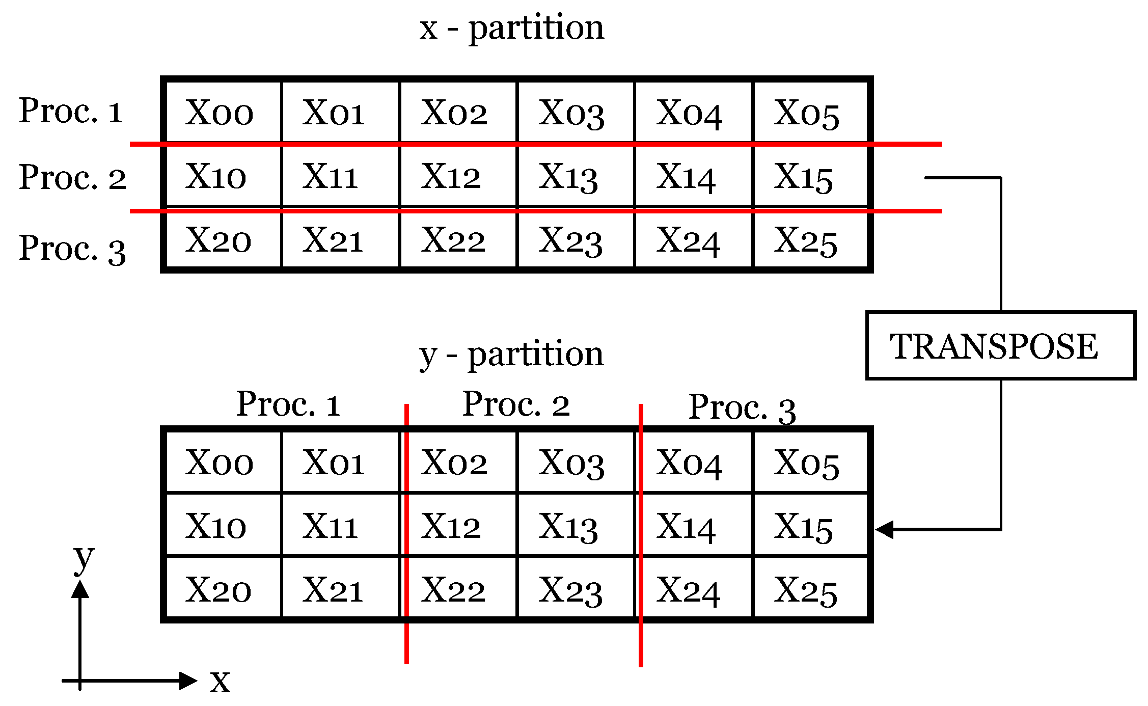
For a simulation run on N_p processors, the full N_x × N_y × N_z domain was first decomposed into N_p parts of size N_x/N_p × N_y × N_z (y-partition) to calculate terms involving y-derivatives or to invert a tri-diagonal system in the y direction. Then, the same domain was divided into N_p parts of size N_x × N_y/N_p × N_z (x-partition) to calculate terms involving x-derivatives or to invert a tri-diagonal system in the x direction (see sketch in Figure 1). The z-derivatives and the inversion of a tri-diagonal system in the z direction can be calculated with the data in either partition. This consideration restricts the way the number of mesh points in each direction can be chosen, given a certain number of processors, because N_x and N_y have to be multiples of N_p. However, this requirement is not overly restrictive.

There are two sets of arrays on each processor: one for the x-partition and the other for the y-partition. Transposing between these two decompositions constitutes the major portion of the inter-processor communication. To keep the inter-processor communication time to a minimum, the code was carefully designed so that the total number of variables to be transposed per iteration was kept at minimum. In this method, all the processor intercommunication is limited to the times when each processor has to communicate with every other processor to complete the reorganization of the data from one domain decomposition to the other. It is essential this processor inter-communication is done in an efficient way for the parallel code to show good scalability. Meanwhile, this method has the very important advantage that there is no need to modify the algorithms used to invert the operators with respect to the ones used in the serial version of the code. Any equivalent parallel algorithm would be, by definition, less efficient than the serial one because it will need some time for processor inter-communication.

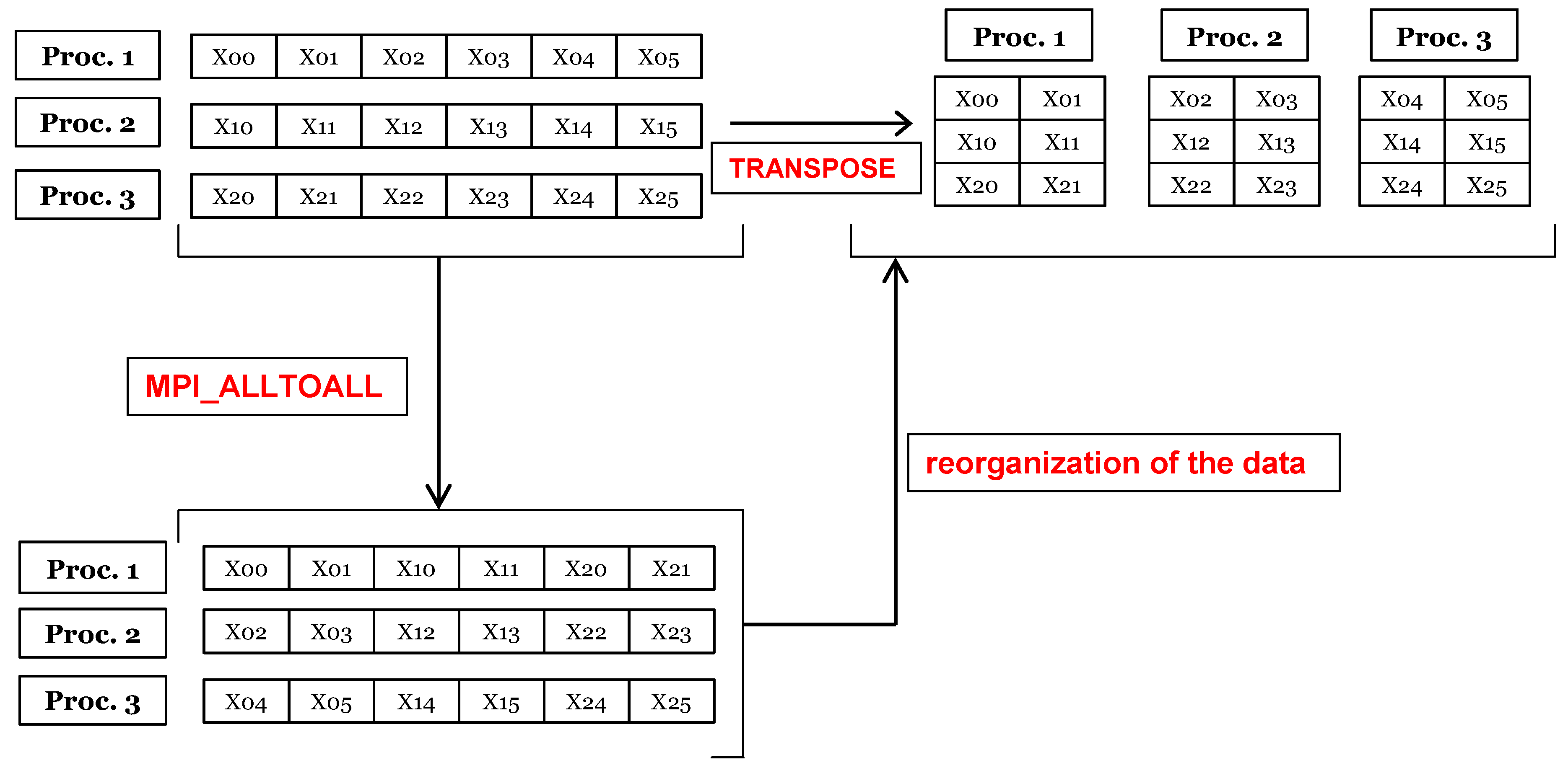
Transposition from the x-partition to the y-partition (and vice versa) was performed using the MPI_ALL_TO_ALL command. This function allows a “scatter” from each process simultaneously. The general structure of the MPI_ALL_TO_ALL operation is given in Figure 2. In this example, each of the three processors holds 1 × 6 vectors. Result of the MPI_ALL_TO_ALL operation is the scatter of data in a certain format so that each processor holds 1 × 6 vectors. At this stage, the correct data are collected by each processor but the data need to be sorted again to be used in the code’s architecture. This operation is labeled in the same figure as “reorganization of the data” which does not require any MPI command because it is internal to each processor. The MPI_ALL_TO_ALL function requires the exchange of information from each processor to all the other processors. MPI_ALL_TO_ALL is a collective operation and each processor should call it, but since the workload is distributed equally among the processors the waiting time is minimized. Another option to perform inter-processor communication is via MPI_ISEND and MPI_IRECV, however we chose MPI_ALL_TO_ALL for ease of implementation.

In a typical Navier–Stokes solver, the main terms are advection, diffusion and pressure terms. Therefore, at least three MPI_ALL_TO_ALL communication is needed in one time step. If any of the turbulence and scalar transport equations are solved in addition, MPI_ALL_TO_ALL communications per time step increases.

The application of this parallelization technique to a code that uses a structured mesh and solves the governing equations in generalized curvilinear coordinates (ξ, η and ζ replace x, y and z, respectively, in the previous discussion) is straightforward. For example, consider a calculation involving summation of derivatives in the three directions in the computational domain. One such example is the calculation of the pressure gradient in the physical x-direction:

$$\partial p/\partial x=(\partial p/\partial \xi )(\partial \xi /\partial x)+(\partial p/\partial \eta )(\partial \eta /\partial x)+(\partial p/\partial \zeta )(\partial \zeta /\partial x)$$

(18)

Consider the calculation of $\partial p/\partial \xi$, $\partial p/\partial \eta$ and $\partial p/\partial \zeta$ terms. The ξ-derivatives should be calculated using the x-partition of the data and the η-derivatives should be calculated using the y-partition of the data. The ζ-derivatives can be calculated in any partition. Here, the y-partition is preferred to estimate them. First, the ξ-derivatives are calculated using the x-partition. This step is done in the following Fortran code:

cccccccccccccccccccccccccccccccccccccccccccccccccccccccccccccccccccccccc subroutine pgrad_x(n,rank) cccccccccccccccccccccccccccccccccccccccccccccccccccccccccccccccccccccccc do 1 k=1,km do 1 j=1,jm do 1 i=2,im-1 l=ln_x(i,j,k,n) dpdc_x(l)=0.5*(qx(l+ic,4)-qx(l-ic,4)) 1 continue return end cccccccccccccccccccccccccccccccccccccccccccccccccccccccccccccccccccccccc

In the above example, “im”, “jm” and “km” are the maximum number of elements in ξ-, η- and ζ- directions respectively with the data in the x-partition, ic is the jump in the index of the 1D array (l = 1 to im*jm*km) corresponding to the neighboring point in the ξ-direction, qx(l,4) is the pressure in the x-partition, dpdc_x(l) is a 1D array containing the pressure derivative in the ξ-direction ($\partial p/\partial \xi$) in the x-partition. After dpdc_x(l) is calculated with the data in the x-partition, it should be transposed to the y-partition. The same variable written in the y-partition is called dpdc_y(l). This transposition is done in the following code:

ccccccccccccccccccccccccccccccccccccccccccccccccccccccccccccc im=img_x(n) jm=jmg_x(n) km=kmg_x(n) do 2111 k=1,km do 2111 j=1,jm do 2111 i=1,im l=ln_x(i,j,k,n) qqt(i,j,k,1)=dpdc_x(l) 2111 continue call transTOy(qqt,qq,1,rank) im=img_y(n) jm=jmg_y(n) km=kmg_y(n) do 2121 m=1,1 do 2121 k=1,km do 2121 j=1,jm do 2121 i=1,im l=ln_y(i,j,k,n) dpdc_y(l)=qq(i,j,k,1) 2212 continue cccccccccccccccccccccccccccccccccccccccccccccccccccccccccccc

Here, two dummy arrays (“qqt”, “qq”) are used to convert the 1D array into a 3D array. Then, the “transTOy” subroutine is used to perform the transposition from the x-partition to the y-partition. Next, one calculates the η- and ζ-derivatives in the y-partition and adds their sum to ξ-derivative of the pressure, now also in the y-partition (one can add two variables only when they are in the same partition). This step is done in the following code:

cccccccccccccccccccccccccccccccccccccccccccccccccccccccccccccccccccccccc subroutine pgrad_y(n,rank) cccccccccccccccccccccccccccccccccccccccccccccccccccccccccccccccccccccccc do 11 k=1,km do 11 i=1,im do j=2,jm-1 l=ln_y(i,j,k,n) dpde(l)=0.5*(q(l+ie,4)-q(l-ie,4)) end do 11 continue do 111 j=1,jm do 111 i=1,im do k=2,km-1 l=ln_y(i,j,k,n) dpdz(l)=0.5*(q(l+iz,4)-q(l-iz,4)) end do 111 continue do 10 l=ls_y(n),le_y(n) pg(l,1)=csi_y(l,1)*dpdc_y(l)+eta_y(l,1)*dpde(l)+zet_y(l,1)*dpdz(l) 10 continue return end cccccccccccccccccccccccccccccccccccccccccccccccccccccccccccccccccccccccc

Here, “im”, “jm” and “km” are the number of grid points in ξ-, η- and ζ-directions, respectively, in the y-partition on a certain processor, “ie” and “iz” are indices necessary to identify the neighboring points needed when estimating the η- and ζ-derivatives in the 1D array in which the 3D variable is written. The variable q(l,4) is the pressure in the y-partition. Finally, csi_y, eta_y and zet_y are the metrics of the transformation written in the y-partition.

In the ADI scheme, at each time level, we have a tridiagonal systems to solve in x, y and z directions in order. In each direction the tridiagonal systems along those grid lines are independent of each other and can be solved independently. Therefore, the tri-diagonal matrix inversion subroutine is another place where transposition between two partitions is needed. The x-sweep in the Thomas algorithm (inversion of a tri-diagonal matrix) should be applied in the x-partition. The y-sweep should be applied in y-partition. The z-sweep can be applied in any partition. Here, the y-partition was preferred. If the x-sweep is done first, the data should then be transposed to the y-partition to perform the y- and z-sweeps and vice versa.

4. Validation Study

As a part of the present parallelization effort, besides the Navier–Stokes solver, the deformable bed module used in simulations with loose beds were also parallelized. The flow, sediment transport and bathymetry at equilibrium conditions were computed with the parallel and serial versions of the code for the case of a 140° curved channel bend of rectangular section studied experimentally by Olesen [15].

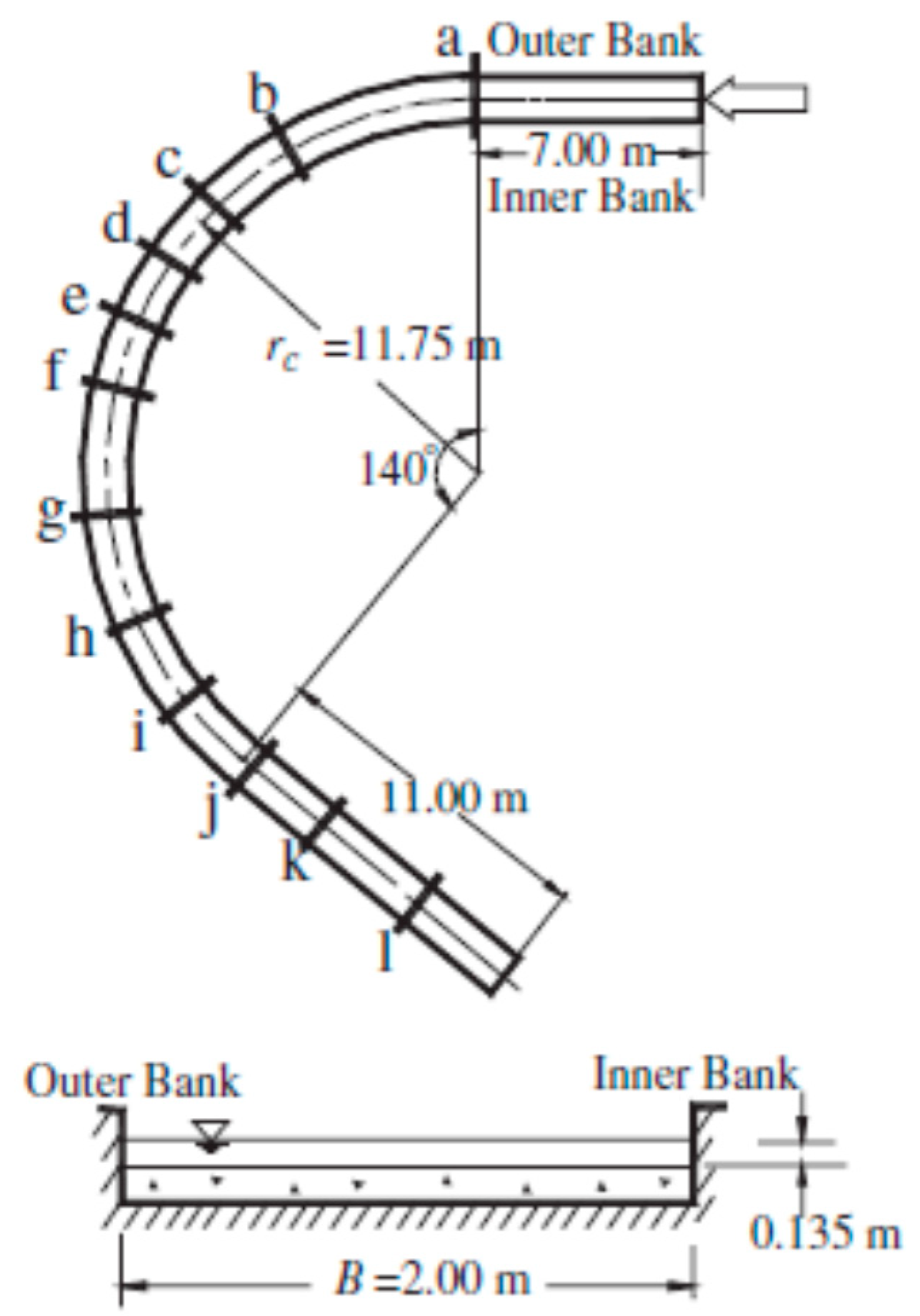
The equilibrium flow, sediment transport and scoured bed in the 140◦ curved bend of rectangular section (Figure 3) studied experimentally by Olesen [15] are computed with both serial and parallel versions of the solver. The curvature radius of the flume in the curved region was r_c = 11.75 m, the width of the channel was B = 2.0 m, and the inflow discharge was 0.118 m³/s. The mean inlet velocity was U = 0.44 m/s and the water depth at the inlet was H = 0.135 m, such that F = 0.38 and R = 59,400. The flume bed was initially leveled with a layer of sand (d₅₀ = 0.80 mm, d₉₀ = 0.9 mm).

The flow was simulated on a computational mesh with close to 350,000 grid points (99 × 101 × 35) using the SA model. Non-dimensional roughness height was close to k+∼900. The side walls were considered smooth. The first points off the side walls and the bed were situated at Δn⁺∼0.7. Fully developed turbulent flow conditions were specified at the inflow section. The experimentally measured value of the bed–load transport rate of 0.0205 kg/m-s was used to specify the inlet boundary condition for bed load transport. As no measurements of the suspended sediment were available, the calculated distribution of the suspended sediment concentration at the outlet was used to specify the mean (laterally averaged) concentration profile at the inlet boundary. The reference level corresponding to the thickness of the bed load layer was assumed to be 2.5% of the inlet channel depth (4d₉₀). This made that 16 mesh points were contained in the vertical direction inside this layer. Bed–slope gravitational force effects were accounted for in all the simulations presented.

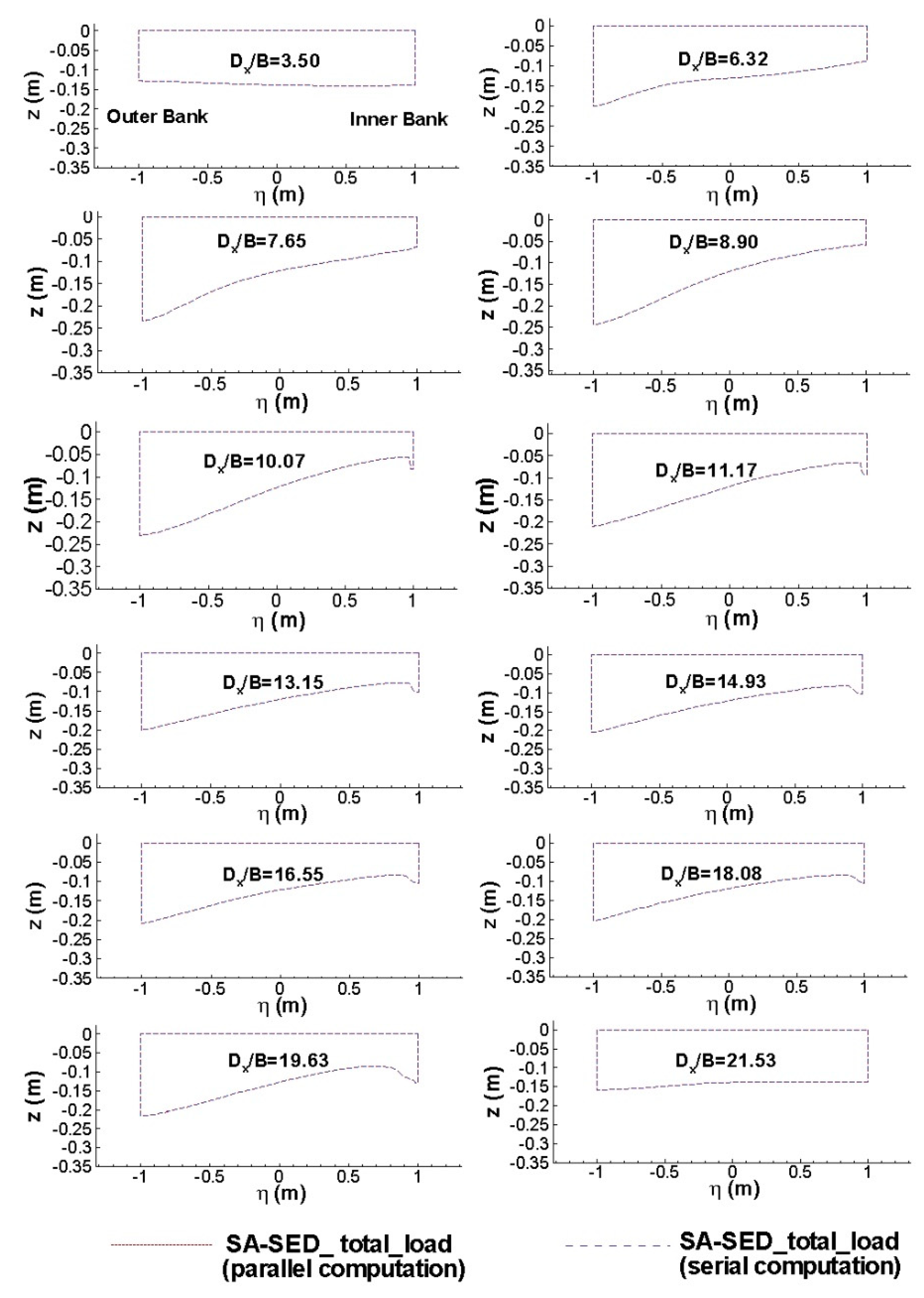
Figure 4 shows the numerical predictions of the water depth levels at relevant sections along the bend. The longitudinal distance D_x is measured along the centerline from the entrance in the straight reach of the channel. The parallel simulation conducted on 8 processors gives exactly the same results as the serial solver.

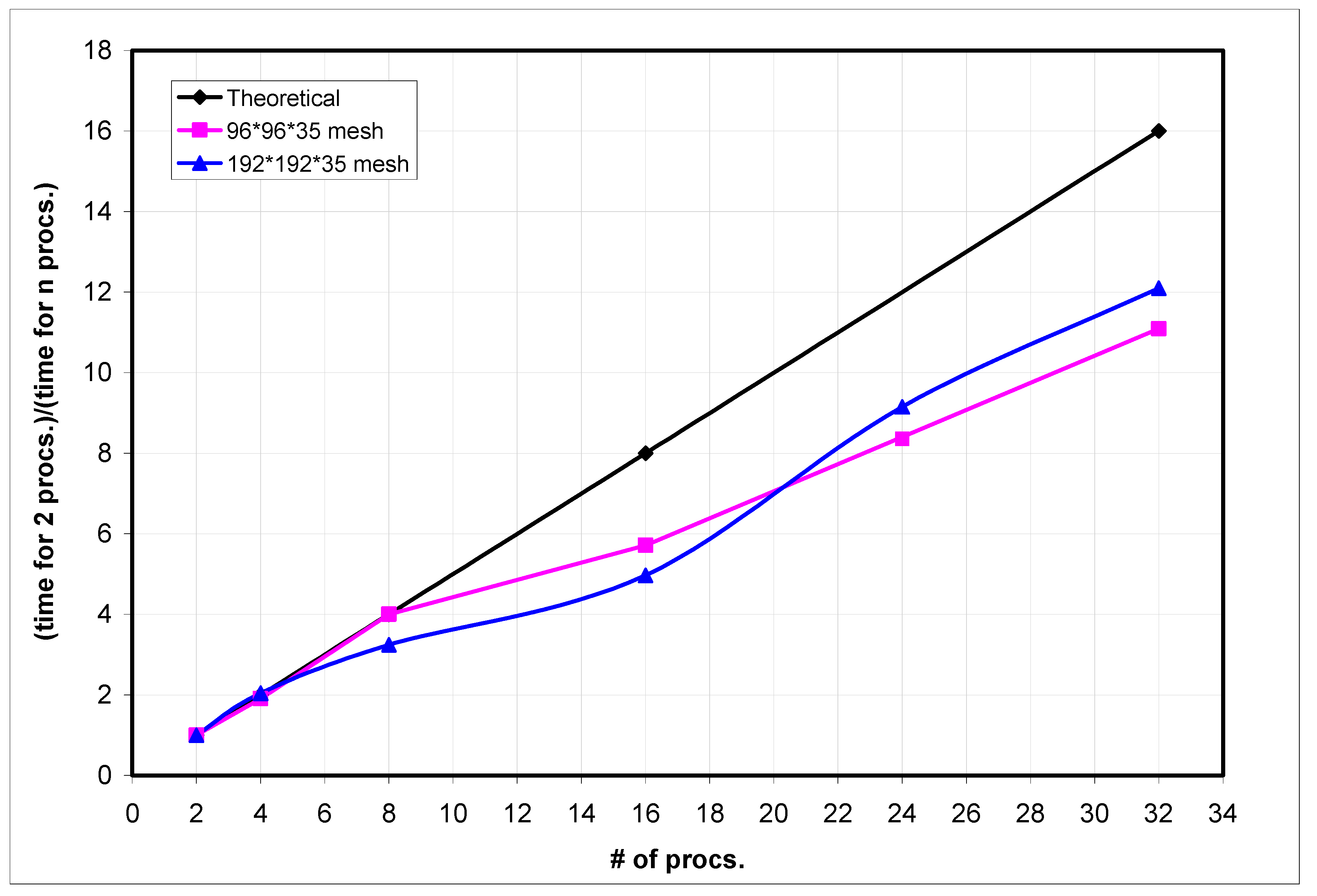
The scalability of the code is analyzed next. Speedup is measured as T(1)/T(n), where T(n) is the execution time of the code on “n processors”. The scalability curve was deduced for the case of the flow in a straight duct. Two different grids containing 322,560 (96 × 96 × 35) and 1,290,240 (192 × 192 × 35) computational points, respectively, were used to assess the code scalability for two characteristic problem sizes. Figure 5 shows the measured speedup for these two different grids. The speedup increased continuously with the number of processors but, as expected, remained below linear scalability. Still, even for the simulations that were run on 32 processors, the scalability of the code was about 70% of the value corresponding to linear scalability. This outcome is considered a very good result. The scalability for the larger mesh problem was superior to the one for the small mesh problem when more than 16 processors were used. This is expected, as for relatively small problems ran on a large number of processors, the processor to processor communication time increases significantly. This results in a decrease in the relative performance of the parallel code. The code was run on one of the IIHR-Hydroscience and Engineering’s cluster, which consisted of 64 nodes with 8 CPUs/node with 16 GB memory per node and processor clock speed of 1.9 GHz.

5. Conclusions

A Navier–Stokes solver that can model bed and suspended sediment transport in 3D on generalized curvilinear coordinated was parallelized in an effort to simulate flow and sediment transport at high Reynolds numbers. The parallelization technique used transposing the computational block to handle derivatives correctly. MPI_ALL_TO_ALL was used to perform transposition. The parallel version of the solver showed good scalability on distributed systems. The parallel 3D Navier–Stokes solver developed in this study for sediment transport calculations in channels can be used in the future to study sediment transport problems in large rivers using large number of processors.

References

- Li, Z.; Wang, C. A fast finite differenc method for solving navier-stokes equations on irregular domains. Commun. Math. Sci. 2003, 1, 180–196. [Google Scholar] [CrossRef] [Green Version]
- Casulli, V. A semi-implicit numerical method for the free-surface Navier–Stokes equations. Int. J. Numer. Methods Fluids 2014, 74, 605–622. [Google Scholar] [CrossRef]
- Kozyrakis, G.V.; Delis, A.I.; Kampanis, N.A. A finite difference solver for incompressible Navier–Stokes flows in complex domains. Appl. Numer. Math. 2017, 115, 275–298. [Google Scholar] [CrossRef]
- Naik, N.H.; Naik, V.K.; Nicoules, M. Parallelization of a class of implicit finite difference schemes in computational fluid dynamics. Int. J. High Speed Comput. 1993, 5, 1–50. [Google Scholar] [CrossRef]
- Wang, H.H. A parallel method for tridiagonal equations. ACM Trans. Math. Softw. 1981, 7, 170–183. [Google Scholar] [CrossRef]
- Sun, X.H.; Zhang, H.; Ni, L.M. Efficient tridiagonal solvers on multicomputers. IEEE Trans. Comput. 1992, 41, 286–296. [Google Scholar] [CrossRef]
- Ma, L.; Harris, F.C., Jr. A Parallel Algorithm for Solving a Tridiagonal Linear System with the ADI Method. In Proceedings of the PDCS 2002, Louisville, KY, USA, 19–21 September 2002. [Google Scholar]
- Constantinescu, S.G.; Squires, K.D. LES and DES investigations of turbulent flow over a sphere at Re=10,000. J. Flow Turbul. Combust. 2003, 70, 267. [Google Scholar]
- Zeng, J. Fully 3D Non-hydrostatic Model to Capture Flow, Sediment Transport and Bed Morphology Changes for an Alluvial Open Channel Bend. Ph.D. Thesis, Department of Civil and Environmental Engineering, The University of Iowa, Iowa City, IA, USA, 2006. [Google Scholar]
- Spalart, P.R.; Allmaras, S.R. A one-equation turbulence model for aerodynamic flows. In Proceedings of the 30th Aerospace Sciences Meeting and Exhibit, Reno, NV, USA, 6–9 January 1992; pp. 5–21. [Google Scholar]
- Spalart, P.R. Trends in Turbulence Treatments. In Proceedings of the 38th Aerospace Sciences Meeting and Exhibit, Reno, NV, USA, 10–13 January 2000. [Google Scholar]
- Arnone, A.; Lıou, M.-S.; Povınellı, L.A. Integration of Navier-Stokes equations using dual time stepping and a multigrid method. AIAA J. 1995, 33, 985–990. [Google Scholar] [CrossRef]
- Chang, K.; Constantinescu, G.; Park, S. Assessment of predictive capabilities of detached eddy simulation to simulate flow and mass transport past open cavities. J. Fluids Eng. 2007, 129, 1372–1383. [Google Scholar] [CrossRef]
- Zeng, J.; Constantinescu, G.; Weber, L. A 3D non-hydrostatic model to predict flow and sediment transport in loose-bed channel bends. J. Hydraul. Res. 2008, 46, 356–372. [Google Scholar]
- Olesen, K.W. Experiments with Graded Sediment in the DHL Curved Flume; Report R 657-XXII M1771; Delft Hydraulic Laboratory: Delft, The Netherlands, 1985. [Google Scholar]
Figure 1.
Definition sketch of x- and y-partitions.
Figure 2.
Transposition of data from one partition to another using MPI_ALL_TO_ALL command.
Figure 3.
General experimental layout of the 140° curved channel bend studied by Olesen [15] showing flume layout and cross-sections where water depths were measured (retrieved from Zeng et al. [14]).
Figure 4.
Comparison of parallel and serial computations of scoured bed in a curved channel.
Figure 5.
Speed-up of the parallel computation under different mesh sizes.
© 2020 by the author. Licensee MDPI, Basel, Switzerland. This article is an open access article distributed under the terms and conditions of the Creative Commons Attribution (CC BY) license (http://creativecommons.org/licenses/by/4.0/).
Share and Cite
MDPI and ACS Style
Kirkil, G. Development of a Parallel 3D Navier–Stokes Solver for Sediment Transport Calculations in Channels. Computation 2020, 8, 84. https://0-doi-org.brum.beds.ac.uk/10.3390/computation8040084
AMA Style
Kirkil G. Development of a Parallel 3D Navier–Stokes Solver for Sediment Transport Calculations in Channels. Computation. 2020; 8(4):84. https://0-doi-org.brum.beds.ac.uk/10.3390/computation8040084
Chicago/Turabian StyleKirkil, Gokhan. 2020. "Development of a Parallel 3D Navier–Stokes Solver for Sediment Transport Calculations in Channels" Computation 8, no. 4: 84. https://0-doi-org.brum.beds.ac.uk/10.3390/computation8040084
Note that from the first issue of 2016, this journal uses article numbers instead of page numbers. See further details here.