Effect of Computational Schemes on Coupled Flow and Geo-Mechanical Modeling of CO2 Leakage through a Compromised Well


1
National Energy Technology Laboratory (NETL), US Department of Energy, Pittsburgh, PA 15236, USA
2
Pacific Northwest National Laboratory, Richland, WA 99352, USA
*
Author to whom correspondence should be addressed.
Computation 2020, 8(4), 98; https://0-doi-org.brum.beds.ac.uk/10.3390/computation8040098
Submission received: 25 September 2020
/
Revised: 4 November 2020
/
Accepted: 9 November 2020
/
Published: 13 November 2020
(This article belongs to the Special Issue Computational Models for Complex Fluid Interfaces across Scales)
Abstract
:Carbon capture, utilization, and storage (CCUS) describes a set of technically viable processes to separate carbon dioxide (CO2) from industrial byproduct streams and inject it into deep geologic formations for long-term storage. Legacy wells located within the spatial domain of new injection and production activities represent potential pathways for fluids (i.e., CO2 and aqueous phase) to leak through compromised components (e.g., through fractures or micro-annulus pathways). The finite element (FE) method is a well-established numerical approach to simulate the coupling between multi-phase fluid flow and solid phase deformation interactions that occur in a compromised well system. We assumed the spatial domain consists of a three-phases system: a solid, liquid, and gas phase. For flow in the two fluids phases, we considered two sets of primary variables: the first considering capillary pressure and gas pressure (PP) scheme, and the second considering liquid pressure and gas saturation (PS) scheme. Fluid phases were coupled with the solid phase using the full coupling (i.e., monolithic coupling) and iterative coupling (i.e., sequential coupling) approaches. The challenge of achieving numerical stability in the coupled formulation in heterogeneous media was addressed using the mass lumping and the upwinding techniques. Numerical results were compared with three benchmark problems to assess the performance of coupled FE solutions: 1D Terzaghi’s consolidation, Liakopoulos experiments, and the Kueper and Frind experiments. We found good agreement between our results and the three benchmark problems. For the Kueper and Frind test, the PP scheme successfully captured the observed experimental response of the non-aqueous phase infiltration, in contrast to the PS scheme. These exercises demonstrate the importance of fluid phase primary variable selection for heterogeneous porous media. We then applied the developed model to the hypothetical case of leakage along a compromised well representing a heterogeneous media. Considering the mass lumping and the upwinding techniques, both the monotonic and the sequential coupling provided identical results, but mass lumping was needed to avoid numerical instabilities in the sequential coupling. Additionally, in the monolithic coupling, the magnitude of primary variables in the coupled solution without mass lumping and the upwinding is higher, which is essential for the risk-based analyses.
1. Introduction
Since the advent of the industrial revolution, the atmospheric concentration of carbon dioxide (CO2) has gradually increased, which is considered as an important criterion for the global warming. [1]. Carbon capture, utilization, and storage (CCUS) has been proposed as a technically viable approach to help reduce anthropogenic CO2 emissions [2]. Once captured from industrial point sources and compressed to a dense phase, CO2 can be transported for geologic storage in depleted hydrocarbon reservoirs, coal beds, deep saline aquifers, or other geologic targets [3]. Successful implementation of geologic carbon storage (GCS) requires effective containment of large volumes of injected CO2 for long periods of time, and it is necessary to ensure that natural and engineered seals serve as effective barriers to unwanted fluid migration. The integrity of active and abandoned wells is also an important aspect of containment assurance [4,5].
The presence of a micro-annulus or crack in the cement sheath of a well system can compromise the effectiveness of a well as a barrier to unwanted fluid migration [6] in GCS, geothermal energy production, oil and gas exploration and production, geologic energy storage, hazardous waste disposal, and other engineered geologic systems. For the well integrity in GCS, zonal isolation is the key concept that is achieved by a well-functioning barrier between the steel casing and the formation rock [7]. However, the cementing operation is the most influential factor for establishing integrity. During the hydration process and cement curing, due to the entrapped air or an inappropriate cement formulation, weak porous space formation may create pathways for existing fluids migration.
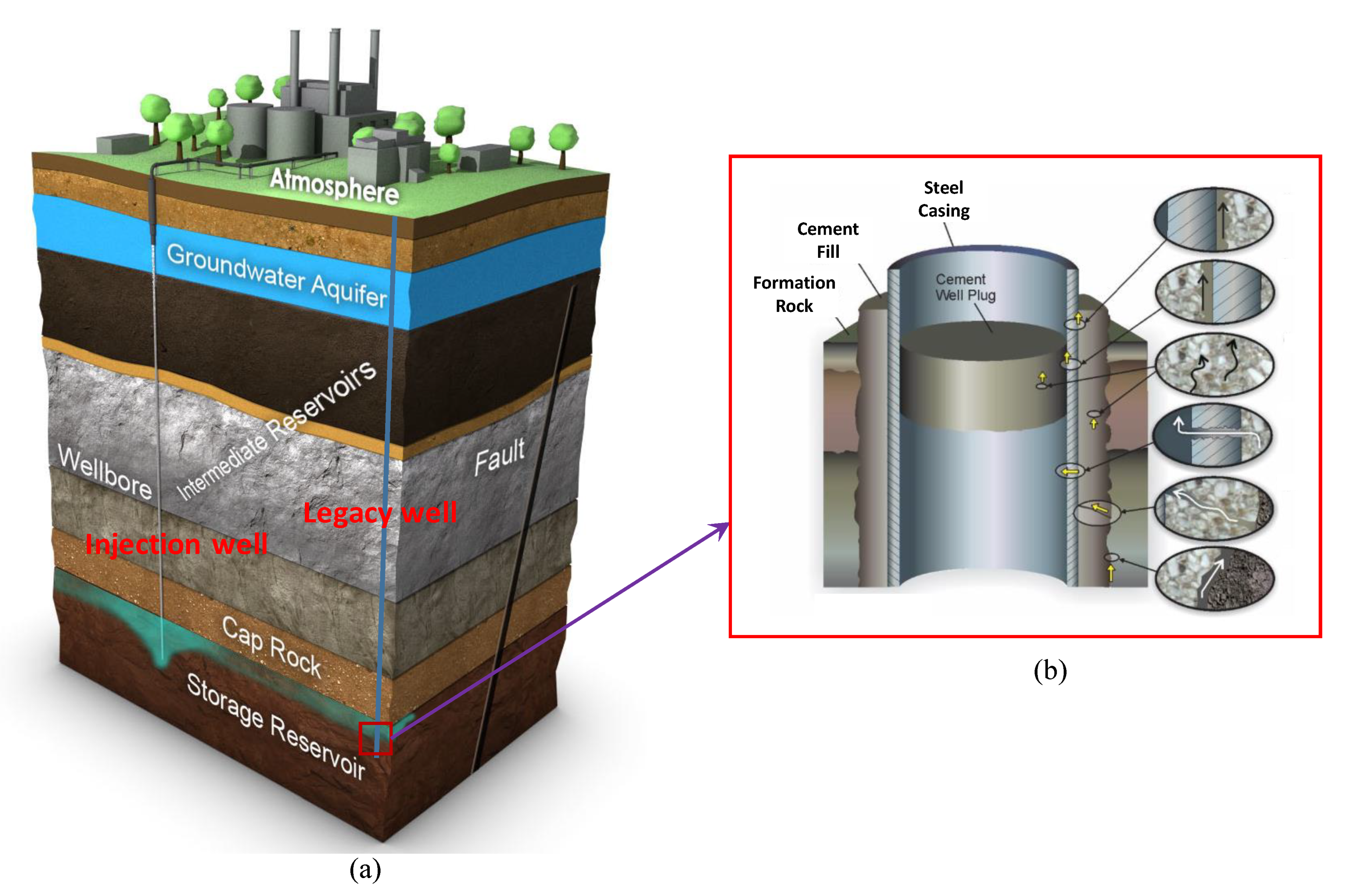
In a compromised well several possible leakage pathways can manifest. Gasda et al. [8], Celia et al. [9], and Wang and Taleghani [10] highlighted six possible reasons for cement sheath failure: (i) crack along the radial direction, (ii) plastic deformation during the hardening phase, (iii) separation between the steel casing and the cement, (iv) separation between the cement and the formation rock, (v) poor cement jobs, and (vi) formation of channel or annulus. Figure 1 presents a representative illustration of an injection well, a compromised legacy well, and possible pathways for fluids leakage through a compromised well.
Well stability failure requires expensive structural remedial operations and a contamination prevention action plan (EPA [11]). Cavanagh et al. [12] reported that in the United States alone, the annual estimated remedial work cost for cement failure is over $50 million a year. In addition, Dusseault and Jackson [13] reported that the estimated remedial cost in British Columbia, Canada is $8 million. Therefore, compromised well, its mechanism, short and long-term effect, and possible prevention are an active field of research. Fluids (e.g., CO2, brine) may migrate through the annulus or crack in the compromised well. Due to fluids flow, inside the porous mediums, fluids pressure develops, which also impacts geo-mechanical aspects of wells [14]. In addition, in the compromised well, the fluids flow, fluids saturation state change, their pressure evolution, and the associated deformation flow are considered as a complex coupled problem, which is the motivation of the present research.
In this paper, for the FE simulations of a field case in Figure 1, we assume that the compromised well geometry consists of a storage reservoir, cement sheath, and steel casing. In addition, we consider a horizontal fracture as a leakage path. Additionally, we interpret that the inside of the well is filled with cement, which represents a plugged and abandoned well. Therefore, the flow problem presented herein calls for simulation of coupled multi-phase hydro-mechanical response in a complex heterogeneous media.
The literature describes some field cases for CO2 injection, like, the Ketzin Pilot project (Chen et al. [15]). The numerical complexities of these types of cases are similar to the Liakopoulos experiments [16]. In addition, among others, Lewis and Schrefler [17] demonstrated associated numerical issues in a homogeneous media. Three-phases (solid, liquid, and gas) finite element simulation in deformable heterogeneous mediums with fractures presents numerical convergence challenges. Helmig [18] demonstrated the computational complexities of modeling fluid flow experimental results in heterogeneous sand mediums reported by Kueper and Frind [19]. The literature reports multiple sources for the numerical instabilities in the multi-phase heterogeneous domains, including: non-linearity of coupled partial differential equations which hold the complex mediums (Binning and Celia [20]), coupling mechanisms of fluids and solids (e.g., the monolithic coupling or the sequential coupling) (Kolditz et al. [21]), and selection of fluids’ primary variables (the capillary pressure plus the gas pressure or the liquid pressure plus the gas saturation) (Helmig [18]). Additionally, for the standard FE, the mass matrices of variables are calculated at each quadrature point, while fluids flowing in porous media, the time derivative of variables are evaluated at nodes (Zienkiewicz et al. [22]). There are notable numerical complexities for the two fluids flow simulation, when (i) one fluid phase approaches to the residual saturation, (ii) the mobility term becomes zero, or (iii) the role of compressibility is substantial. For cases with three-phases heterogeneous mediums, selection of (i) numerical solvers (linear and non-linear solvers), (ii) time integration scheme (implicit, explicit, or automatic time stepping), (iii) preconditioner (Jacobi type or Incomplete Lower Upper (ILU) factorization type or without preconditioner), and (iv) memory storage (symmetry or asymmetry) are crucial issues to obtain numerical convergence (Chen et al. [23]).
Work described herein seeks to address those challenges for the scenario of leakage through a compromised legacy well in a GCS system. Using the finite element method, we tested two coupling mechanisms, and two sets of fluids primary variables and considered their contribution to numerical instabilities. For the fluids flow, the primary variables are (i) the capillary pressure and the gas pressure (PP scheme) and (ii) the liquid pressure and the gas saturation (PS scheme). We also use Brooks and Corey [25] model to account for the transition between the wetting phase fluid and the non-wetting phase fluid. We also introduced the mass lumping and the upwinding techniques (see Helmig [18]) to assess the numerical stability in the heterogeneous mediums. Moreover, to verify the performance of finite element simulations, we compared our FE results with the analytical solutions of Terzaghi’s 1D consolidation (see also Coussy [26]), Liakopoulos [16] laboratory test and Kueper and Frind [19] experimental results. We conducted these comparisons to assess the accuracy in the coupled FE solutions and to investigate the effect of fluids’ primary variables on the heterogeneous interface with relevance to the case of leakage through a compromised legacy well. In addition, the problem statement in the benchmark solutions are relevant to compromised well. The purposes of our present investigations are to (i) assess the risk of CO2 leakage through observation points including in the fracture zone, (ii) monitor coupled geo-mechanical responses due to CO2 injection, and (iii) investigate the effect of coupling scheme (e.g., monolithic and sequential coupling) with and without the mass lumping and the upwinding algorithms on the coupled finite element solutions of CO2 leakage.
An open-source solver named OpenGeoSys [27] was used for finite element modeling. The Gmsh [28] was used for mesh generation. In the following sections, we will discuss details of governing equations, coupled finite element formulations, benchmark solutions, and coupled finite element model of a compromised legacy well.
2. Governing Equations
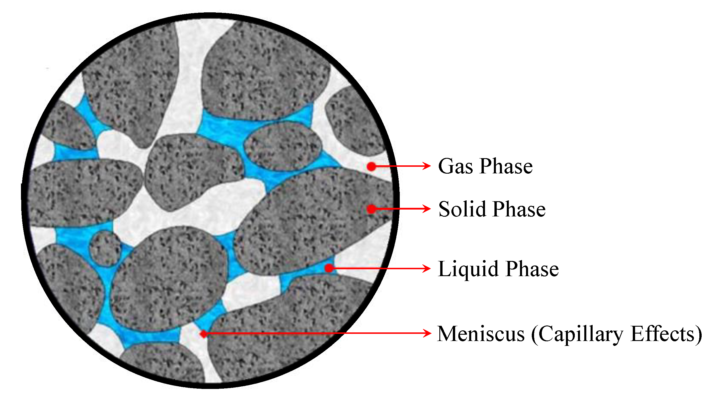
Considering the average-representative theory (Bear and Bachmat [29]), we present herein the momentum conservation, the mass conservation for the multi-phase flow type model. We assume that the modeled system is composed of porous rock media with fluids (gas and liquid) saturating the pore space such that the system comprises three phases (). In addition, we ignore components of each phase (e.g., vapor or solid deposition), and geochemical interactions. The phases are the gaseous or the non-wetting phase ( = g), the liquid or the wetting or the aqueous phase ( = l), and the solid phase (), which we illustrate in Figure 2. We also assume that the porous media adheres to the “average volume” theory, and the individual phases are distributed over the “control volume” (de Boer [30]). Pores of the porous mediums are filled with fluids (i.e., liquid and gas). The three phases of the system are considered as a mixture, with two-phase fluid flow coupled with the deformation flow for two sets of fluids primary variables combining the “mixture theory” (Truesdell [31]), and the “volume fraction” theory (de Boer [30]). In the following section, we present the balance equations.
2.1. Momentum Conservation Equations
We assume that (i) the porous medium satisfies the quasi-static equilibrium condition and in the isothermal equilibrium state. Therefore, we ignore the acceleration term. (ii) The porous medium also supports the Newton’s third law. Thereby, the interaction force of the solid and the fluid are equal but have an opposite sign. As a result, the interaction forces cancel each other, and we ignore them. (iii) The porous medium also follows the small deformation theory.
Considering the assumptions mentioned above, we present the momentum conservation equation as
where, is the total stress tensor, which is the summation of phases, is the density of mediums, which also holds the summation convention of phases (see Bear and Bachmat [29]), is the gravitational acceleration, which is acting in the vertical direction. In addition, we present the details of constitutive laws of , and the linear momentum conservation equation in Appendix A.
2.2. Mass Balance Equation
We assume that (i) there is no exchange of mass between the solid and the fluids. Thereby, we ignore the geochemical interactions. (ii) The solid phase satisfies the isotropic condition. (iii) Fluid phases are immiscible. (iv) The porous medium satisfies the compositional approach (see Panday and Corapcioglu [32]). Therefore, the mass balance equation is the summation of the associated phase of balance equations.
Considering the aforementioned assumptions, we obtain the mass balance equation as
In Appendix A, we discuss details of the constitutive relations for the mass balance equations. The final form of the momentum equation and the balance equation for a given physical problem depends on many factors (see Aziz and Settari [33]). However, in this paper, we limit our discussion to two essential conditions. They are (i) the selection of fluids primary variables: the PP scheme and the PS scheme, and (ii) assumptions of constitutive relations for coupled solutions. To avoid the repetition of similar equations, we first present a general form of the coupled equation (see Appendix A, Equations (A5) and (A17)). Then, we obtain the PS scheme and the PP scheme for our numerical solutions as follows.
The PP scheme:
The PS scheme:
In Equations (3)–(8), to obtain the “well posed” (see Peiro and Sherwin [34]) coupled finite element solutions, we have a total of 34 Equations for 34 variables (see Appendix A and Table A1 and Table A2).
In addition, in Equations (3)–(8), we can summarize the second-order partial differential equations (SOPDE) under three headings depending on conditions (see also Chen et al. [23]). For example, if the multiplication of coefficients of the SOPDE is greater than zero, it becomes elliptic. The equation behaves parabolic or hyperbolic, if the multiplication of coefficient is zero or less than zero, respectively. For the two-phases flow equations, when the phase mobility is zero, the total mobility becomes positive. Therefore, the pressure equation is treated as elliptic. Again, while one of the fluids phase density varies (see also Helmig [18]), the equation becomes the parabolic. Moreover, when the capillary pressure term is zero, the equation becomes hyperbolic. To solve such a complex coupled SOPDE solution, there are different approaches, e.g., Implicit Pressure, Explicit Saturation (IMPES), and the Implicit method (see Gundersen and Langtangen [35]).
In this paper, for a coupled numerical solution, we use two types of numerical solvers. They are (i) the library of iterative solvers (Lis) for the linear system: SpBICGSTAB type solver (see Chen et al. [23]), and (ii) for the non-linear solution: PICARD type solver (see Paniconi and Putti [36]). In addition, for the coupling of two fluids and solid, we use (i) the monolithic coupling and (ii) the sequential coupling. In the first case, we solve the governing equations concurrently using one solver. In contrast, in the latter case, we obtain a solution of similar equations using distinct solvers. In the solution scheme, we use the ILU type preconditioner and the asymmetric storage (see also Saad [37]). In addition, we consider the saturation and the displacement error threshold as 1 × 10⁻³ and 1 × 10⁻⁵ m, respectively, while a similar magnitude for the pressure is 1 Pa. For the convergence, we consider the relative error criterion (see also Chen et al. [23]).
3. Coupled Finite Element Formulations
We introduce the weak formulations, and the Galerkin finite element method in the governing equations to obtain the finite element solution (see also Zienkiewicz et al. [22]). In the matrix notation, the coupled algebraic equations for the two-phase flow, and the deformation can be written as
In Equation (9), in general, and are the non-symmetric matrices which depend on solution vectors, . is the time derivative of . is the time-dependent function for the gas pressure, the capillary pressure, and the displacement. Additionally, and are known as the “mass matrix” and the “coefficient matrix”, while demonstrates the Neumann boundary terms. It is worth mentioning that we show Equation (9) for the PP scheme only to avoid similar equations.
Details of matrix elements in Equation (9) can be found in Lewis and Schrefler [17].
There are different approaches to solve Equation (9) (see Wood [38]). However, herein, we use the —method. In addition, following the finite difference method, the time discretization of Equation (9) can be written as
where, is the integration parameter. and are vectors corresponding to the time and , respectively. Additionally, and represent the previous and present time steps, respectively. We also assume that the initial state of solution vectors , at an initial time are known.
For the coupled hydro-mechanical solutions, the domain is bounded by an arbitrary boundary . In addition, to obtain solutions of unknown variables, we define the initial conditions and the boundary conditions as follows
where, , and are the initial state displacement, capillary pressure, and gas pressure, respectively.
For the above-mentioned primary variables, boundary conditions are given by
where, and are the assigned displacement and tractions, respectively, on the corresponding boundaries and . Additionally, and are the prescribed capillary pressure and the gas pressure, respectively, on the boundaries and . is the unit normal vector. is the assigned fluids fluxes, where represents the liquid and gas phases.
Additionally, for the diffusive fluxes, solutions of coupled non-linear balance equations exhibit the parabolic form. Again, when the diffusive fluxes are small enough compared to the convective fluxes, the governing equations are treated as the hyperbolic form (see also Aziz and Settari [33]). Moreover, the non-linear convective term’s differential operator is not symmetric. In such a situation, if one fluid phase approaches its residual saturation or the mobility term (see Equation (A8)) approaches zero, then the upwinding technique is convenient (see also Helmig [18]). Furthermore, in a heterogeneous porous media, without the upwinding method, the primary variables of the governing equations oscillate strongly, which moreover do not predict fronts perfectly for the convection-diffusion type problem (see also Aziz and Settari [33]). In addition, a finite element domain comprised of composite medium and with coarser mesh, the oscillation is also challenging. We also discuss such an oscillation in the next section. In this regard, possible solutions may be small-time steps and finer mesh, which require additional computational time.
As in the upwinding method, the central difference solution of the second-order partial differential equation with respect to space is replaced with the first-order solution in the direction of fluid flow. Thereby, there is a debate for and against the upwinding method regarding stability and accuracy issues. It is worth mentioning that selection of the upwind method (see also Helmig [18]) is crucial for the solution of multi-phase fluids flow in a porous media. A choice of erroneous algorithms may attempt to withdraw fluid phase from nodal points, where there might not have even fluid (see also Lewis and Roberts [39]). In such a situation, “fully upwinding” method is numerically advantageous than other upwinding method, while in other cases, “fully upwinding” method may require a cutoff to achieve the stability. Thereby, it is worth mentioning that considering the coupling mechanisms of operational processes (e.g., coupled fluids flow and deformation flow), a selection of the upwinding technique is critical. Moreover, without the upwinding method, introducing revised “quadrature rule”, the associated oscillation also can be resolved (see also Lewis and Roberts [39]). However, the computational time in the “quadrature rule” is challenging.
It is worth mentioning that in the Results and Discussions of a Compromised Well section, we present a comparison of with and without the mass lumping and the upwinding method for the monolithic coupling and the sequential coupling. Additionally, in the next section, we demonstrate benchmark solutions of the above discussed coupled finite element formulations.
4. Benchmark Solutions
4.1. Terzaghi’s 1D-Consolidation
Terzaghi’s 1D consolidation theory [40] is considered as the necessary foundation of the coupled hydro-mechanical, and the liquid flow through the porous media. In this section, we compare the analytical solutions of Terzaghi’s 1D consolidation with the finite element model. In this regard, we assume that the porous medium is fully liquid saturated; the medium is in the isotropic state, and homogeneous. Additionally, we consider the single drainage (see also Terzaghi [40]). The analytical solution for the Terzaghi’s 1D consolidation is available in many textbooks (see also Coussy [26]). In this section, considering Murad and Loula [41], we obtain the analytical solutions for the pore pressure and the effective stress as follows
where, , , , , are non-dimensional quantities. is the effective vertical stress, is the pore-pressure or the liquid pressure, is the initial pore pressure, is the initially assigned vertical pressure, k is the permeability of the porous media, t is the time, is the Young’s modulus, is the Poisson’s ratio, is the liquid viscosity, and is the drainage path.
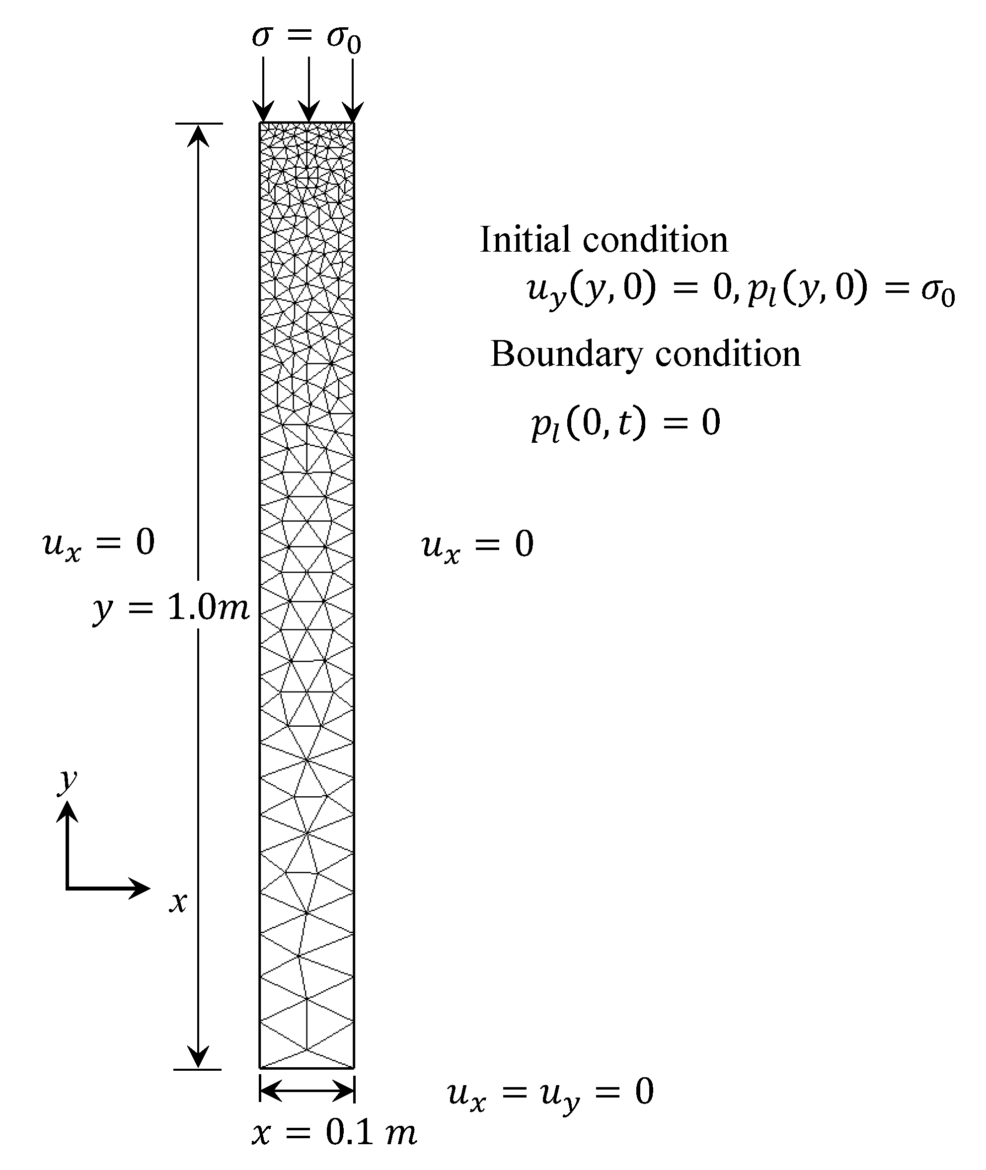
We consider that the height and the width of the porous media are 1.0 m and 0.1 m, respectively (see also Figure 3). For any coupled solution of saturated porous media, there should have two types of boundary conditions. They are the displacement boundary (or similar) and the hydraulic boundary. At the bottom, we restrict the displacement along the horizontal and the vertical direction. Additionally, along the lateral direction, we also limit the horizontal displacement. In addition, along the load application area, we introduced finer mesh and applied a uniform load of 1000 Pa. We perform the simulation in two steps. In the first step, across the top surface, we constrain the drainage. Thereby, due to a sudden application of load, along with the porous medium, uniform pore pressure is developed, which is equivalent to the applied load. At this stage, only the liquid pressure carries the applied external pressure, and the effective stress is zero. In the second step, the top surface is open and permeable. Additionally, the lateral boundaries are also impermeable. In Figure 3, we demonstrate the initial and the boundary conditions, while in Table 1, we present model parameters.
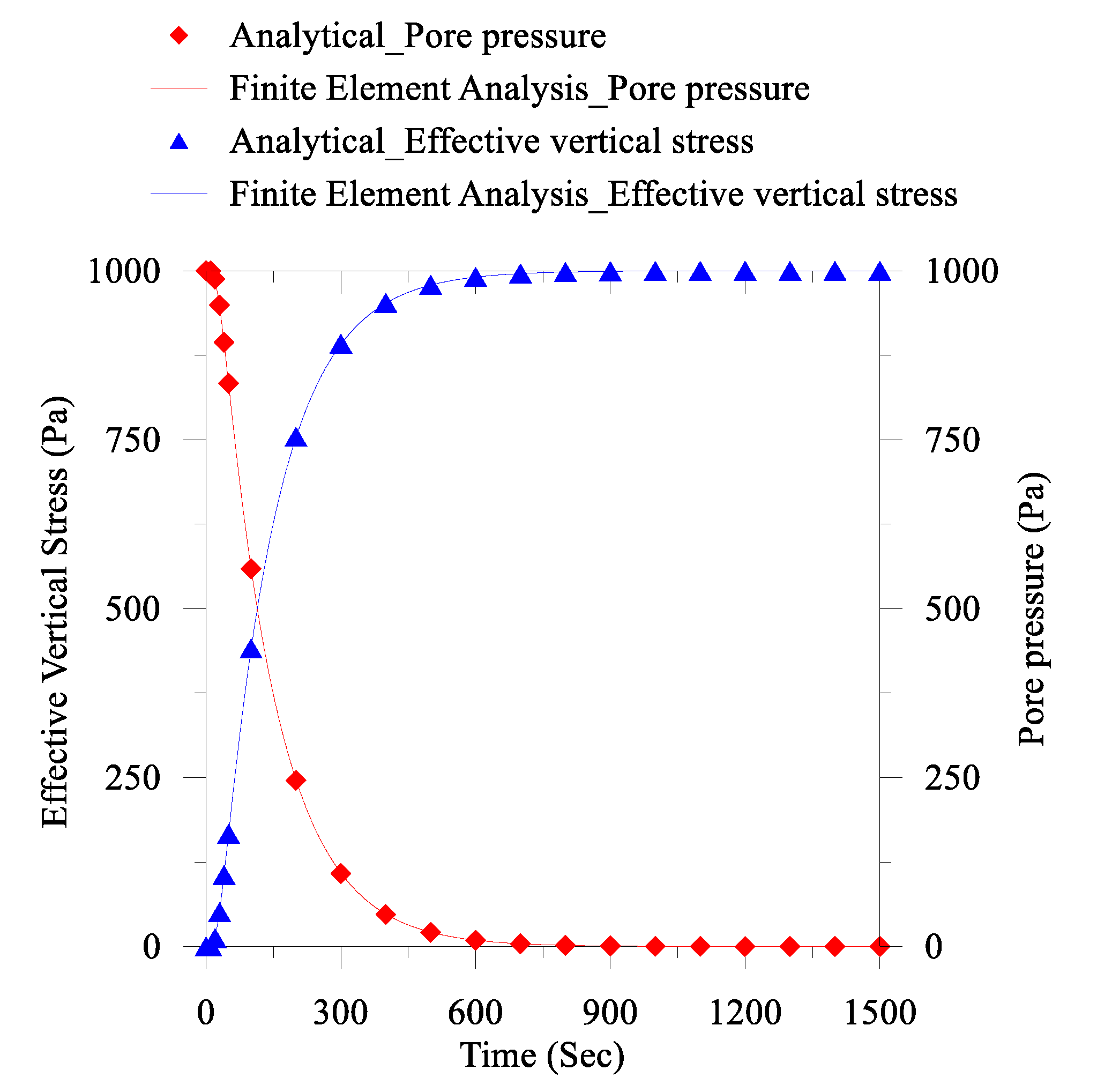
It is noteworthy that the 1D consolidation process in the porous media behaves like a diffusion method. At the initial stage, the liquid pressure/pore pressure and the effective stress are relatively high. Therefore, we also consider a small-time step during the simulation. We present a comparison of the analytical and the finite element solutions in Figure 4, which represents a good agreement. Additionally, we observe that the liquid pressure/pore pressure dissipation results in increasing the effective vertical stress. Moreover, when the pore pressure decrease with respect to time is negligible, the effective vertical stress increment rate is also minimal (see also Figure 4).
4.2. Liakopoulos Test
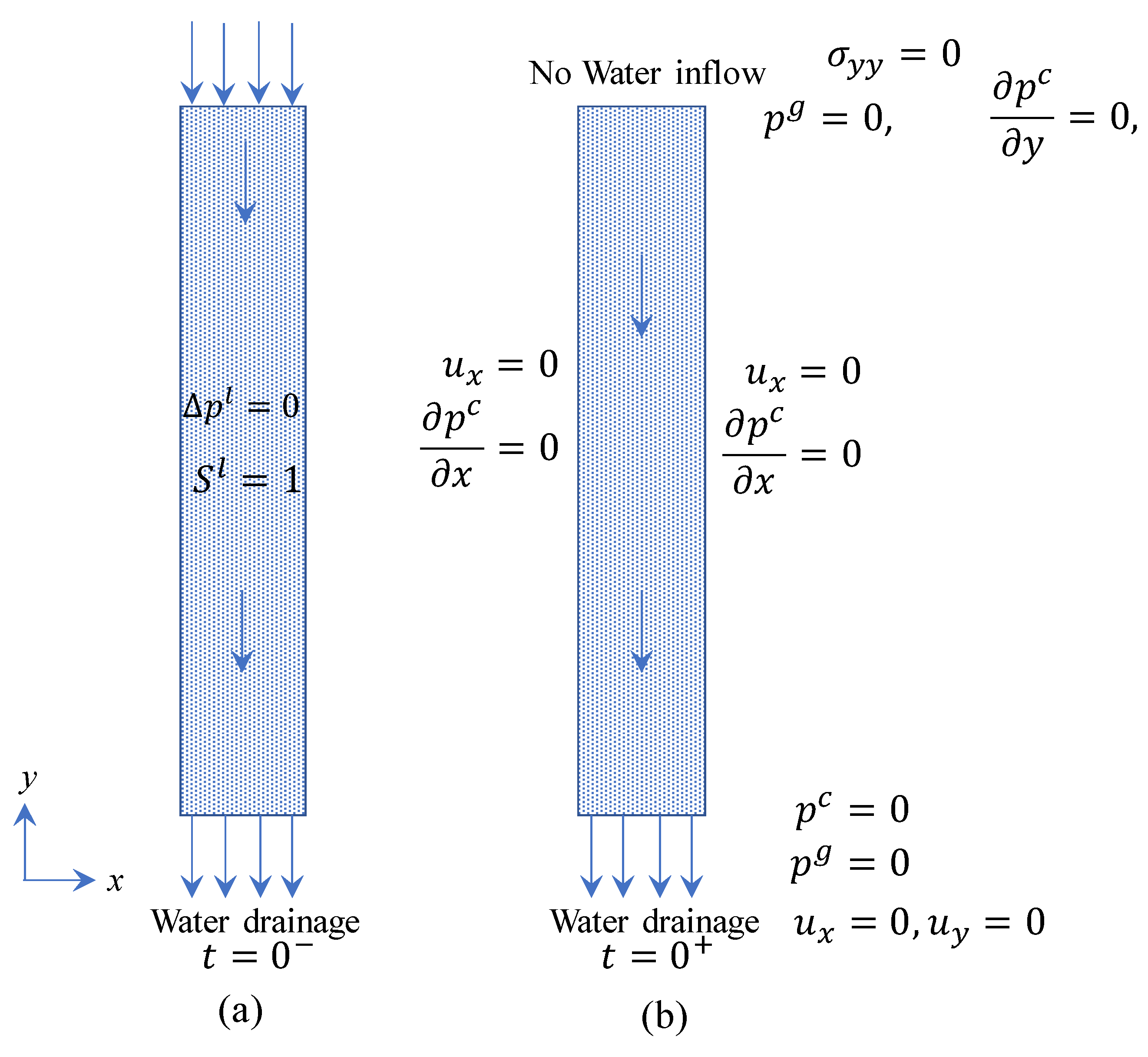
In the above section, for the 1D Terzaghi’s consolidation representing the two-phases saturated media, we discussed a comparison of the analytical solution with the finite element results. In contrast, in this section, we present a comparison analogy of the Liakopoulos experiments (see also Liakopoulos [42]) showing three-phases media, with finite element solutions. Liakopoulos [42] performed experiments on a 1.0 m Perspex column filled with the Del Monte sand and instrumented using the tensiometers to measure the pore pressure change along with the column height (see Figure 5). The purpose of such a test is to investigate the fully saturated condition (e.g., two-phases media: solid phase and the liquid phase, with the liquid saturation = 1) to the gradual desaturation state development (e.g., three-phases media: solid phase, the liquid phase, and the gas phase). During the test, only the gravitational force is considered for the consolidation process. In the Liakopoulos test, initially, constant flow through the column is continued, and free drainage is also allowed at the bottom through a filter to ensure the initial water pressure gradient is zero. At the bottom, after achieving the uniform flow condition , the liquid flow supply is terminated () at the top so that only due to the gravitational force, the accumulated liquid in the medium could escape. Additionally, Liakopoulos [42] presented the measured values of the tensiometer readings and the outflow rate.
We present details of the model parameters in Table 2. In addition, we perform two types of finite element solutions. In both cases, we consider an identical condition, which also provided the opportunity to compare model performances of two solutions with the experimental results. In the first case, we couple two-phases fluids flow with the deformation flow. In the latter case, we also couple the Richards solution [43] with the deformation flow. For the deformation flow, we consider the poroelasticity (see Coussy [26]). It is worth noting that for the Del Monte sand Liakopoulos [42] performed laboratory tests to obtain the porosity and hydraulic properties. Liakopoulos did not present the mechanical properties of sand. However, among others, Lewis and Schrefler [17] back-calculated the Young’s modulus and the Poisson’s ratio. Comparing with hydraulics properties test results in Liakopoulos [42] experiments, Lewis and Schrefler [17] also presented the capillary pressure and the saturation relations (see Table 2), which are valid for the liquid saturation greater than 0.91. In addition, considering the Brooks and Corey [25] model, we obtain the relative permeability for the gas phase from Lewis and Schrefler [17].
To maintain the similarity with the Liakopoulos test, we assume that (i) the consolidation happens only due to the gravity force along the vertical direction, (ii) the medium is in the equilibrium state, (iii) in the initial state, the medium is fully saturated, then the desaturation started from the top. We also illustrate the boundary conditions in Figure 5.
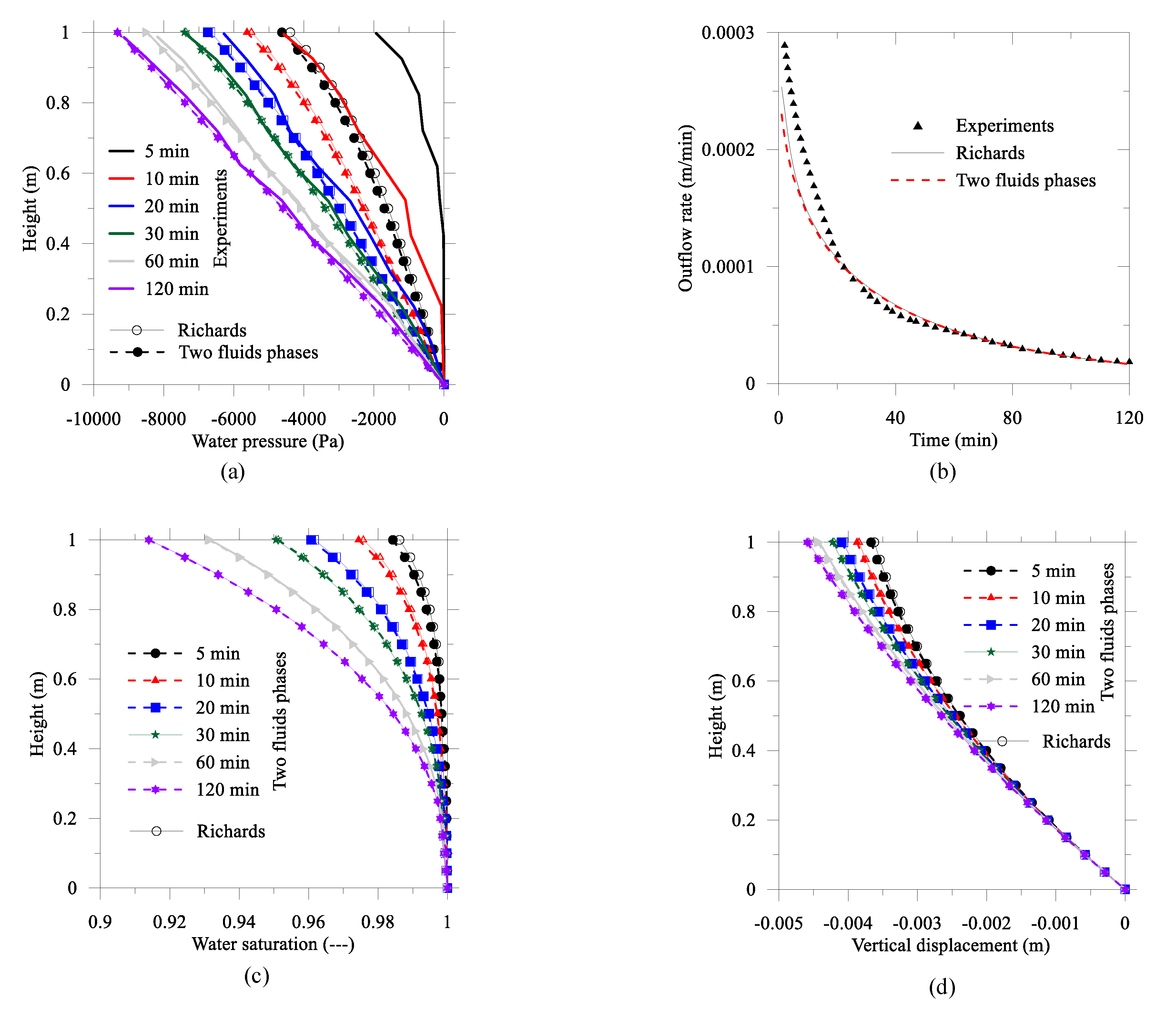
Liakopoulos [42] only measured the liquid pressure profile and the fluid outflow rate through the bottom for time. Due to the unavailability of the Liakopoulos experimental data for the capillary pressure and saturation, a comparison of the finite element results is not possible. In Figure 6a, we compare the water pressure measurement with the two fluids phases and the Richards flow. We observed that before 30 min, predicted finite element (FE) results for the water pressure decreased rapidly compared to the experimental measurement. Among others, Schrefler and Scotta [44] also observed a similar phenomenon. After 30 min, both FE results match well with experimental results. In Figure 6b–d, we also present results for the water outflow rate at the bottom, the water saturation profile, and the vertical displacement profile, respectively. For the identical conditions and material properties, the two fluids’ phases result has good agreement with the coupled Richard flow [43].
4.3. Kueper and Frind Test
In the above two benchmark solutions, we present a homogeneous medium for two phases and three phases. However, in this section, we present a heterogeneous medium for the benchmark comparisons, and the mechanisms are closely similar to heterogeneous compromised well problems in the next section.
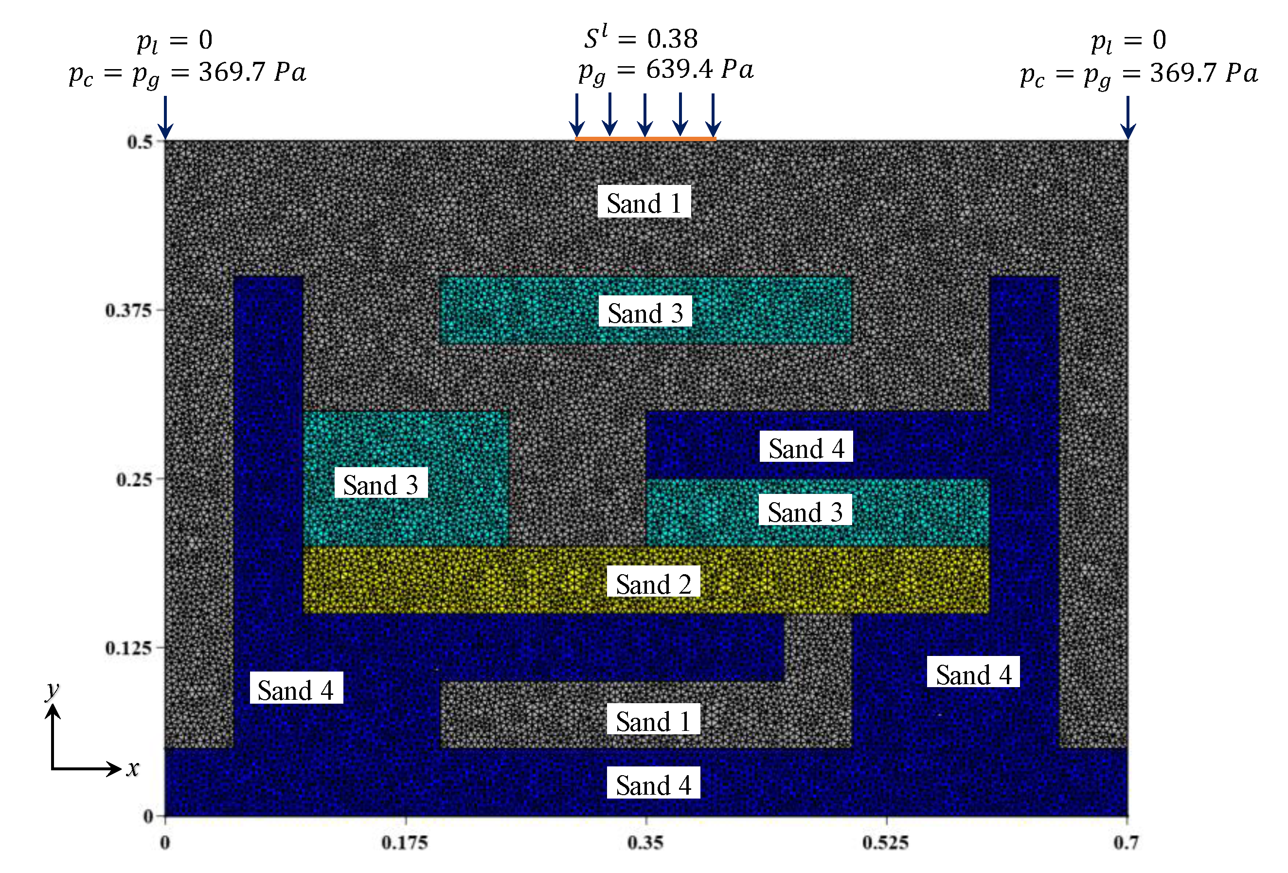
Kueper and Frind [19] performed laboratory experiments to investigate the dense non-aqueous phase liquid (DNAPL, e.g., the tetrachloroethylene) infiltration. An acrylic glass flume of dimension 0.7 m × 0.5 m × 0.006 m (see Figure 7) is filled with four different types of uniformly distributed sand (e.g., sand 1 = # 16 Silica, sand 2 = #25 Ottawa, sand 3 = #50 Ottawa and sand 4 = #70 Silica). Initially, mediums are adequately water saturated. Then, the infiltration is controlled with a constant tetrachloroethylene saturation of 0.38. Additionally, in Figure 7, we present details of the boundary conditions. From Kueper and Frind [19], we demonstrate fluids properties in Table 3 and the Brooks-Corey model parameters in Table 4.
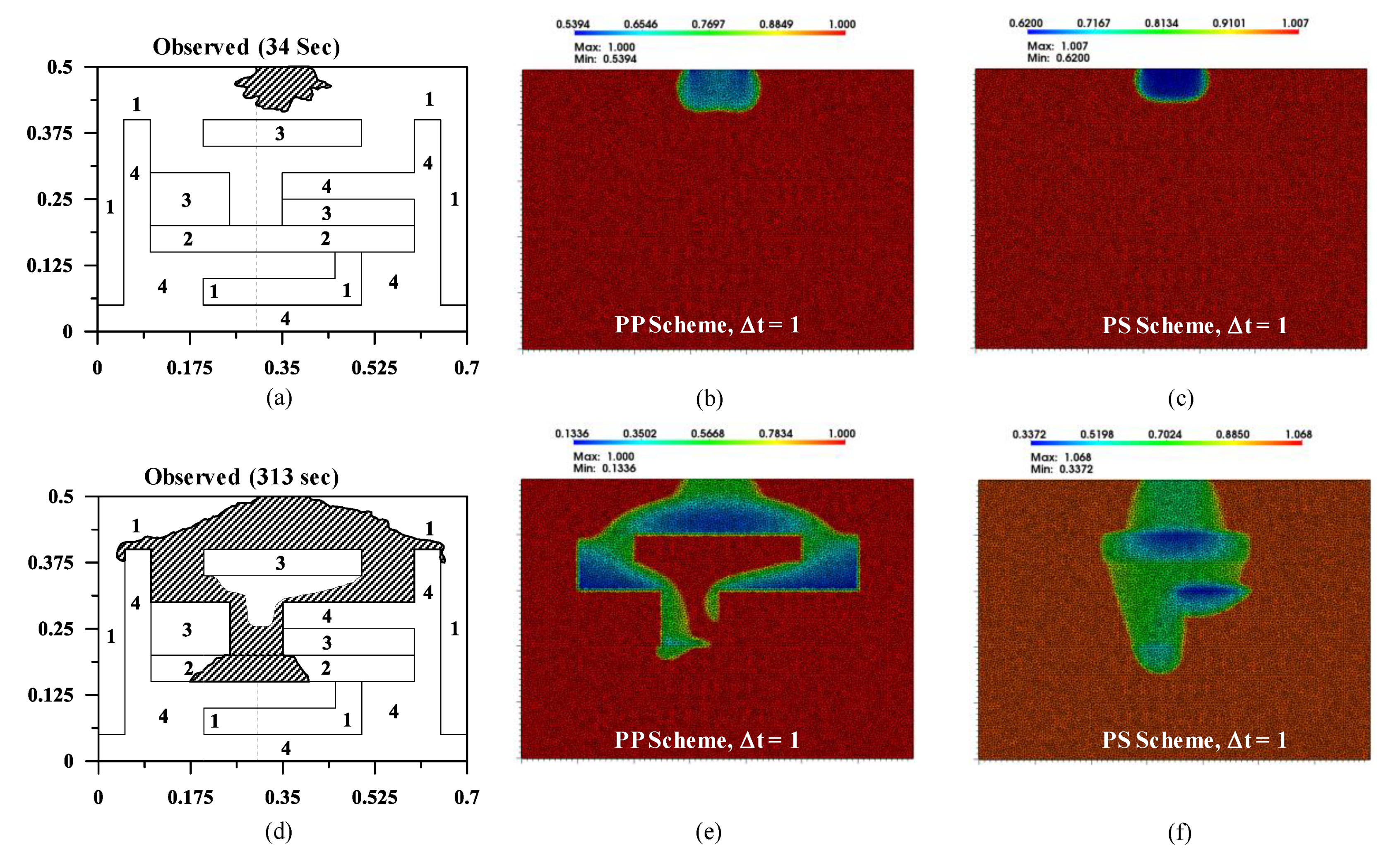
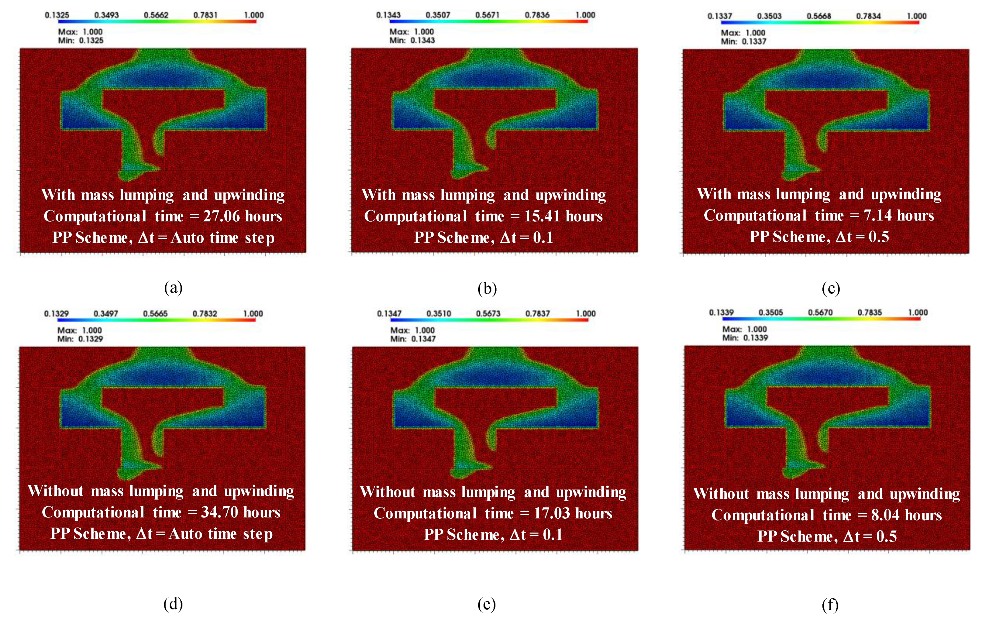
For the finite element (FE) simulation, we use the two-phases model considering two sets of primary variables. They are (i) the capillary pressure and the gas pressure (the PP scheme) and (ii) the liquid pressure and the gas saturation (the PS scheme) (see also Equations (3)–(5) and (6)–(8)). We also include the upwinding and the mass lumping techniques for numerical simulation. For the FE model, we use three nodes of triangular elements. The number of nodes and elements are 18,475 and 37,914, respectively. In Figure 8, we present a comparison of experimentally observed response with numerically predicted tetrachloroethylene infiltration at 34 s and 313 s. The purpose of such a comparison is to investigate the importance of primary variables selection for fluids flow modeling at the interface of heterogeneous composite media. From comparisons in Figure 8, we observe that at 34 s, before the plume reaches to the heterogeneous interface, both numerical schemes (e.g., PP and PS) produce reasonably well plume distribution. However, due to dissimilarities in the hydraulic properties (see Table 4), when plume reaches to the heterogeneous interface at 313 s, we notice a notable difference in the PP scheme and the PS scheme. The PP scheme captures the observed response well compared to the PS scheme. In addition, the accuracy has been compromised in the PS scheme. Moreover, we also observe that heterogeneity has a significant impact on the two-phases fluids flow behavior. In addition, in such a case, the PS scheme provides unphysical fluids flow results. Additionally, we also run a total of eight simulations comparing with and without the mass lumping and the upwinding using different time steps to assess their effect on simulations, which is demonstrated in Table 5.
From Table 5 and Figure 9, we observe that the selection of the mass lumping and the upwinding techniques and the time step significantly impact the computational time. Additionally, to address fluids migration through different material properties in Kueper and Frind [19] test, we also use very fine mesh. Moreover, Kueper and Frind [19] performed the experiment for a shorter time, thereby the effect of with and without the mass lumping and the upwinding methods in the finite element solutions are negligible. However, for a more extended period in well modeling, such an effect is significant. In the next section, for the compromised well, we discuss (i) selection of coupling mechanism effect (ii) with and without the mass lumping and the upwinding methods, and (iii) the effect of injection rate. In addition, in the compromised legacy well modeling section, as we also have a heterogeneous medium; therefore, to avoid the numerical instability in the PS scheme, we consider the PP scheme algorithms for the finite element simulation of fluids migration.
5. Numerical Modeling of Compromised Well
5.1. Geometry and Properties
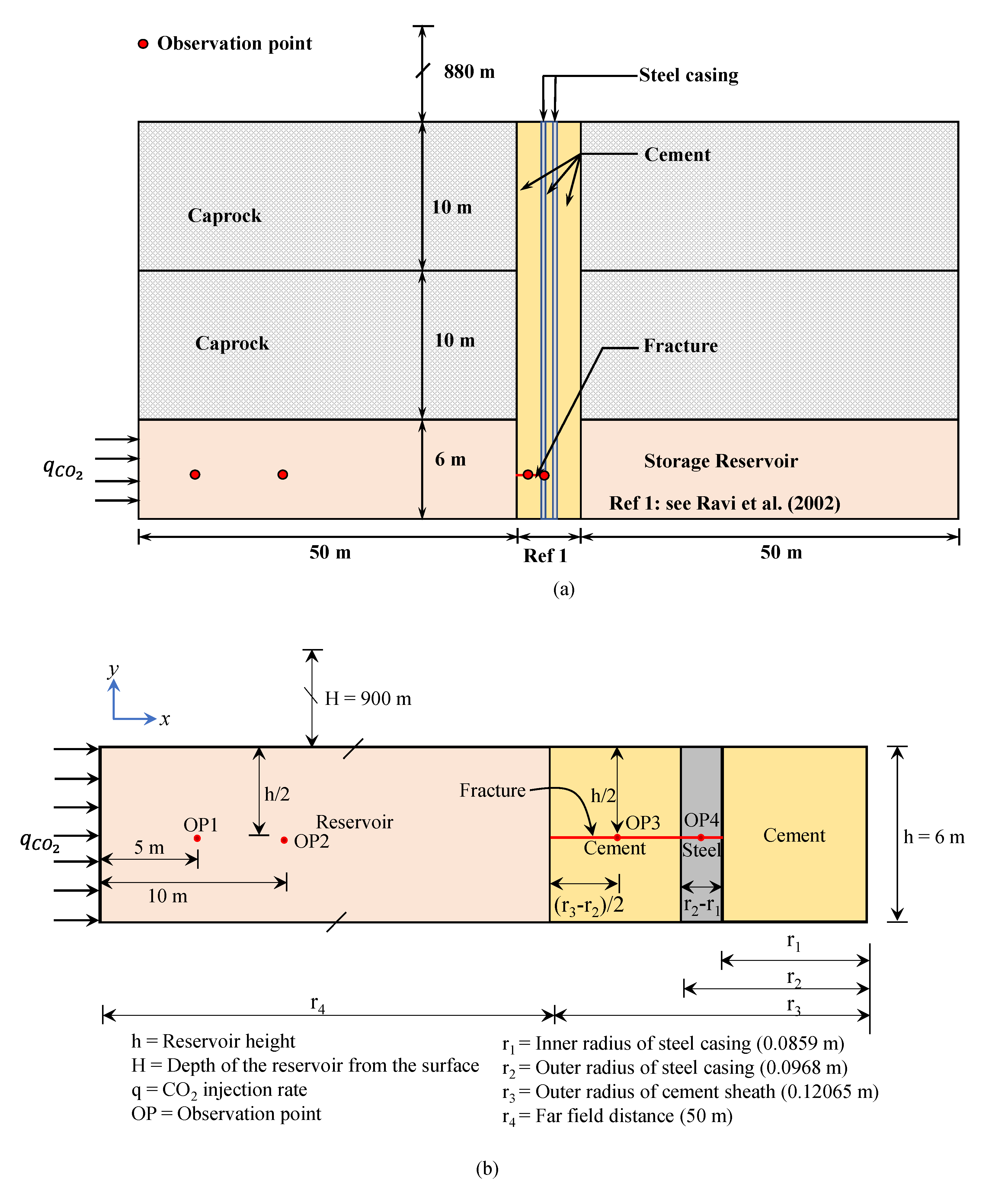
Following Figure 1, we schematically illustrate a compromised legacy well in Figure 10 for coupled finite element (FE) simulations. We assume that the geologic storage medium has two main components. They are (i) a porous CO2 storage reservoir (6.0 m), and (ii) a relatively impermeable caprock (20.0 m) and stress above the caprock. We also assume that the storage reservoir is located 900 m below the surface. It is worth mentioning that we consider a simplified geometry for the coupled FE modeling to reduce the computational time. Thereby, in the numerical model, above the CO2 storage reservoir, we assume the stress state as an overburden pressure (see also Figure 10b). In addition, in Figure 10b, we consider fracture in the left wall of the steel casing, while its right wall is intact. Hence, we also assume that fluid will not flow through the steel wall’s right impervious wall. As a result, in Figure 10b, possible fluid flow paths are compromised fracture zone and the porous medium. Moreover, in Figure 10b, to minimize the right end-boundary effect in the numerical simulation, we extend the longitudinal dimension to 50.0 m on the other side of the CO2 injection face. Theoretically, depending on the injection rate and geophysical properties of the study domain (see Figure 10b), coupled hydro-mechanical responses to any points are proportionate from the fluid injection phase distance. However, such responses in coupled finite element modeling also depend on the selection of the coupled algorithms (see also Figure 8 and Figure 9), which we investigate herein for a compromised well. Therefore, considering the above-mentioned assumptions, we use a total of four observation points in Figure 10b to monitor the coupled hydro-mechanical behavior.
In addition, we obtain the well geometry from Ravi et al. [45] (see also Figure 10b). The diameter of the wellbore is 0.2413 m. The outer diameter and the inner diameter of the casing are 0.1936 m and 0.1718 m, respectively. Thereby, the steel casing thickness is 0.0109 m, which we also assume as an impervious media. Additionally, to mimic the legacy well, we assume that inside of the well’s steel casing is sealed using cement. Moreover, the cement thickness between the legacy well’s outer wall and the steel casing is 0.02385 m. We also assume the fracture aperture is 625 μm, which allows fluids migration through cement porous media. We ignore the fracture propagation. We present material properties of casing, reservoir, cement, and fracture in Table 6.
We assume that the study domain is in the quasi-continuum condition, and in the equilibrium state. We also assume that the average density of the overburden medium is 2650 kg/m3. In addition, we consider the domain’s temperature is 34 °C and in the isothermal state. With such a stress state and temperature condition, we obtain corresponding fluid properties from the National Institute of Standards Technology webbook (NIST [46]), and we present them in Table 7. Additionally, to account for the transition of the wetting phase to the non-wetting phase, we consider the Brooks and Corey model, which we demonstrate in Table 8.
5.2. Initial Conditions and Boundary Conditions
We consider that the vertical stress , the minimum horizontal stress , and the maximum horizontal stress are acting along the y-axis, z-axis, and x-axis, respectively. We also assume that the ratio between the horizontal stress ( and ) to the vertical stress is 0.8. During the initial state, we also obtain the “geostatic” condition due to the gravity force. Additionally, in Table 9, we present the initial stress conditions.
To assign the boundary condition, we restrict fluids flow along the bottom, right, and top of the domain. In Figure 10b, we present CO2 injection boundary on the left side. We introduce fluids saturation in terms of the capillary pressure. To maintain the quasi-static condition, we assume small-time incremental and a constant CO2 injection rate, so that we may avoid any disturbance during CO2 injection. Additionally, at the top and the bottom of the domain, we restrict the vertical displacement. We also consider that along the horizontal direction (x-axis), the CO2 injection face (see Figure 10b) is movable. In contrast, we assume another front of the horizontal direction is the fixed boundary by restricting the displacement.
6. Results and Discussions of a Compromised Well
6.1. Effect of Coupling Mechanisms
In Figure 8 and Figure 9, we demonstrate the selection of multi-phase flow algorithms and coupling mechanisms on the accuracy of the results in heterogeneous porous media. In this section, we extend our study to a compromised well, which is also a heterogeneous media and holds a similar complexity as we noticed in the benchmark validation for Kueper and Frind [19] test. In addition, we found in Figure 8 and Figure 9 that in the interface layer of two different porous media, the selection of multi-phase flow primary variables has a significant effect on the results and computational time.
In our compromised legacy well geometry, we have four different sets of material properties (see also Table 6), and the study domain is relatively more complicated compared to Kueper and Frind [19] test. Additionally, when fluid phases front pass through an interface layer of storage reservoir-cement or cement-steel or steel-cement (inside the well) or through the horizontal fracture (see also Figure 10b), it is challenging to obtain numerical stability. In addition, we assume that the steel is impervious to fluid transport. Therefore, during finite element mesh generation using Gmsh [28], for each material properties (see Table 6), we introduce four sub-domains. To couple multi-phase fluids flow and deformation flow, we implement the domain deactivation technique (see also Zienkiewicz, Taylor, and Zhu [22]) for the steel, so that steel does not participate in the fluids phase interchange, and to behave as an impervious medium. Such a technique is required because the steel domain or impervious medium makes it difficult and at some points impossible to obtain numerical stability due to the convergence problem.
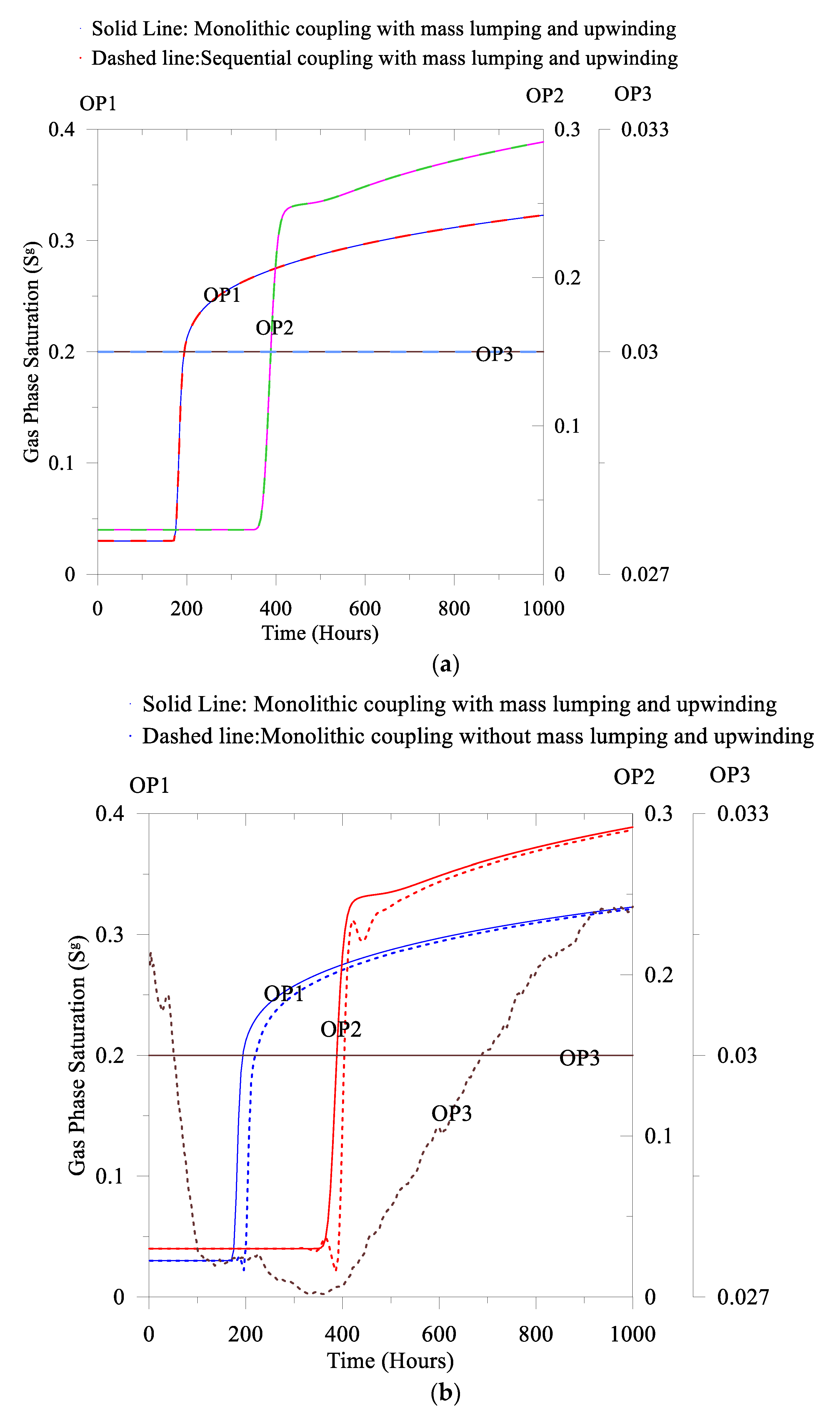
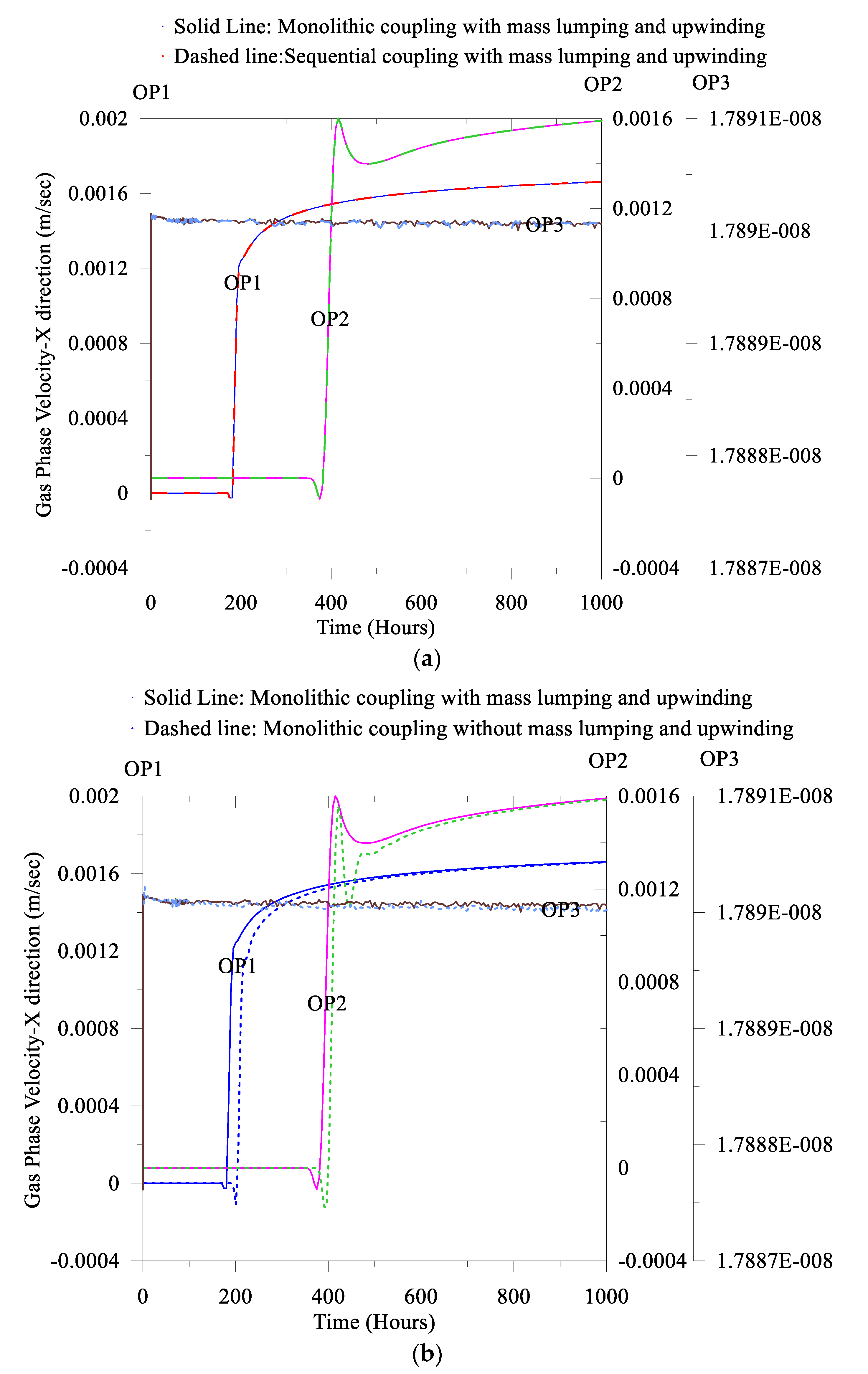
To address the effect of coupling mechanisms in the multi-phase porous media, we consider two different types of coupling for Figure 10b. They are the monolithic coupling and the sequential coupling. Additionally, we also introduce the mass lumping and the upwinding methods (see also Zienkiewicz, Taylor, and Zhu [22]; Helmig [18]) to comprehend their effects in the coupling processes. Additionally, we consider four observation points: OP1, OP2, OP3, and OP4 in Figure 10b.
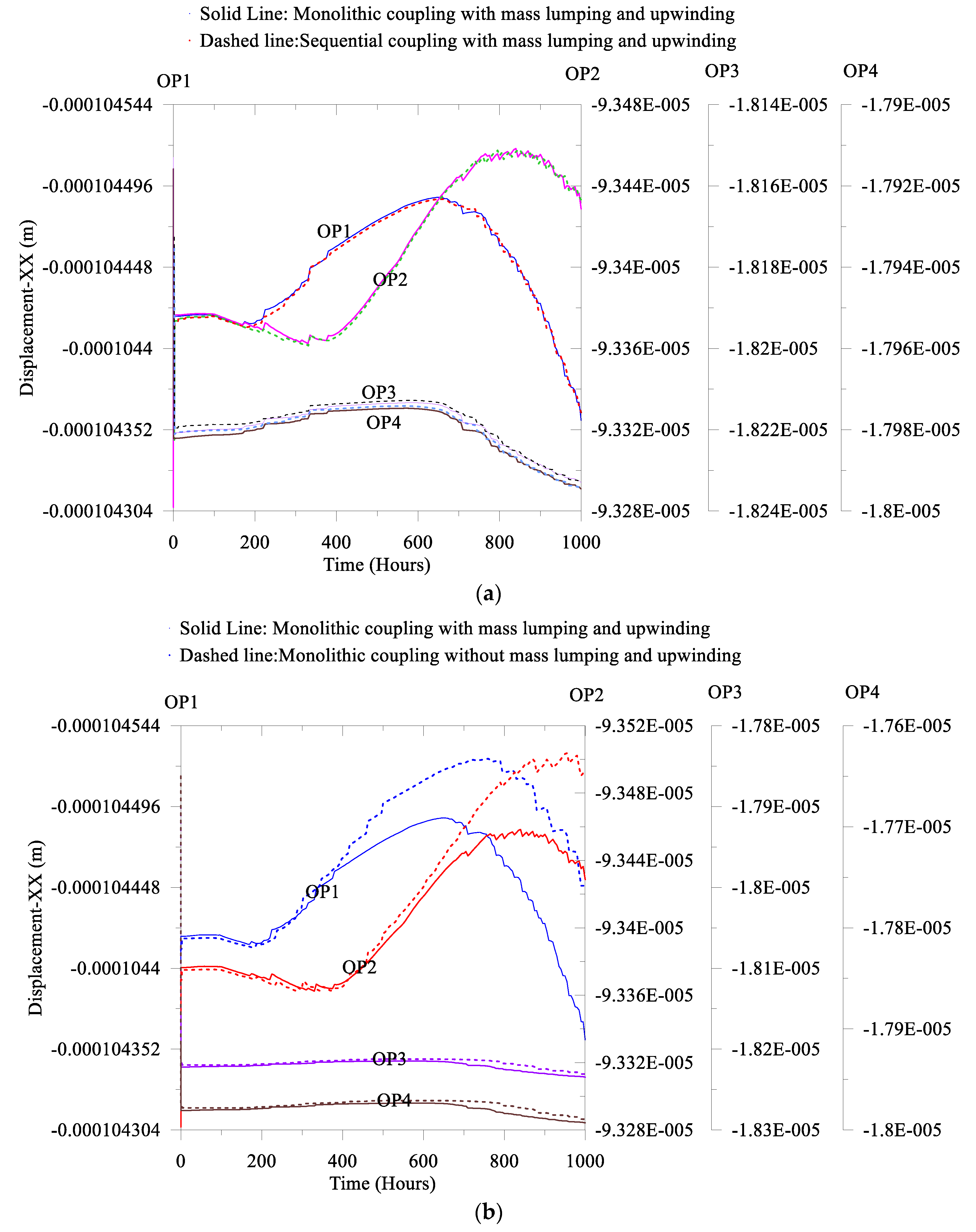
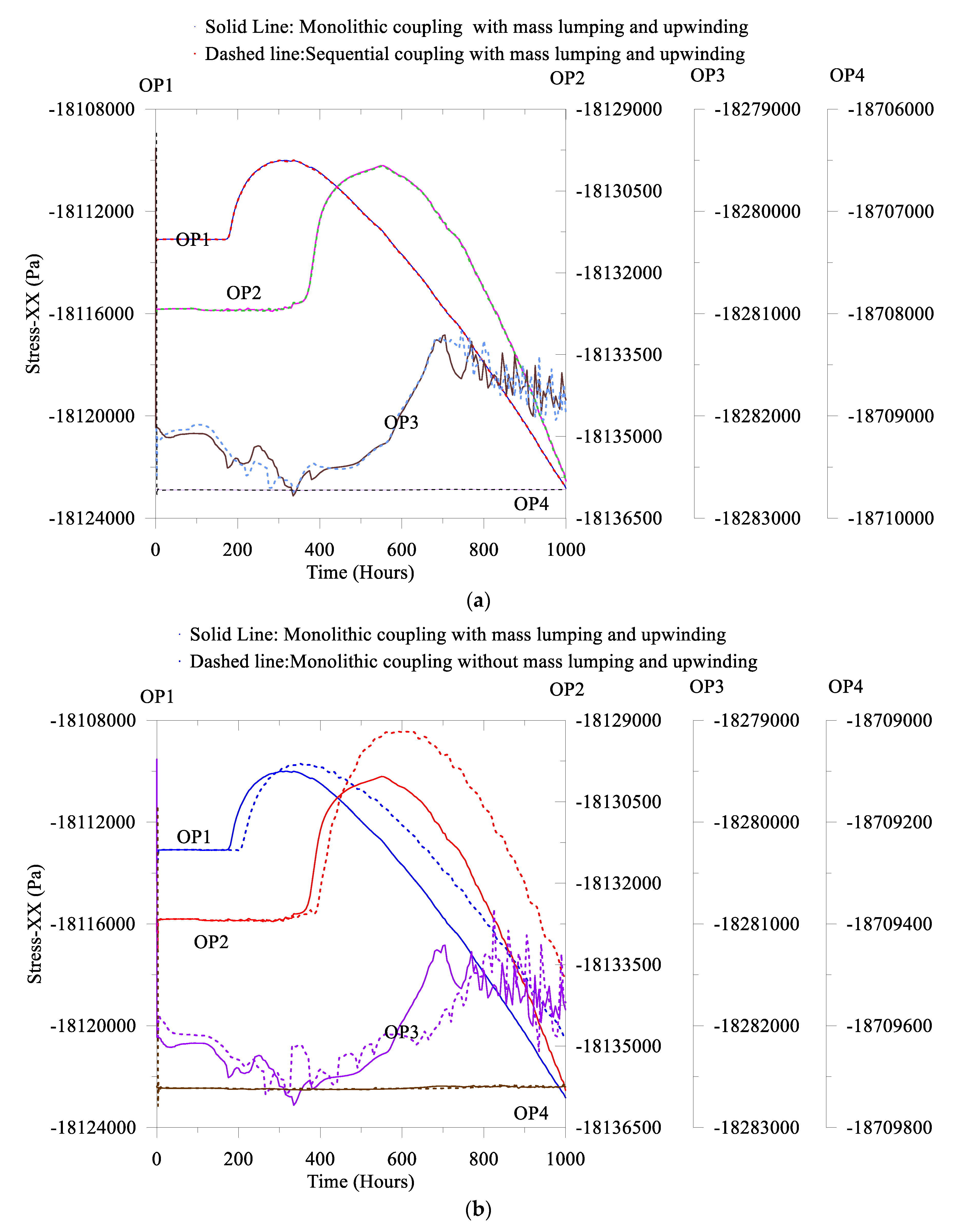
In Figure 11a, we observe that with the mass lumping and the upwinding, both couplings provide almost identical results. However, without the mass lumping and the upwinding, in the sequential coupling endures the convergence problem. Additionally, in Figure 11b, we also compare the monolithic coupling with and without the mass lumping and the upwinding, which demonstrate a notable effect in the predictions. It is worth mentioning that in the compromised well, to assess the risk, it is desirable to predict the maximum worst-case through the observation points. In addition, from Figure 11 and Figure 12, we find that without the mass lumping and the upwinding, for each primary variable, the maximum magnitude is relatively high. We also notice a similar response in Figure 13 and Figure 14 for the gas phase saturation and the gas phase velocity. Additionally, for Figure 13b and Figure 14b, we notice that along the fracture without the mass lumping and the upwinding, the numerical solution experiences notable prediction differences of the gas phase saturation and the gas phase velocity. Therefore, it is evident that for the risk base compromised well analyses, careful consideration is essential to select coupling mechanisms, the mass lumping, and the upwinding.
It is worth mentioning that to select coupling mechanisms, the mass lumping, and the upwinding, the most critical three criteria are the accuracy of the results, the numerical convergence, and the computational time. In addition, we discussed earlier the possible solutions to overcome such complexities for the benchmark validation (see Section 4).
6.2. Effect of the Injection Rate
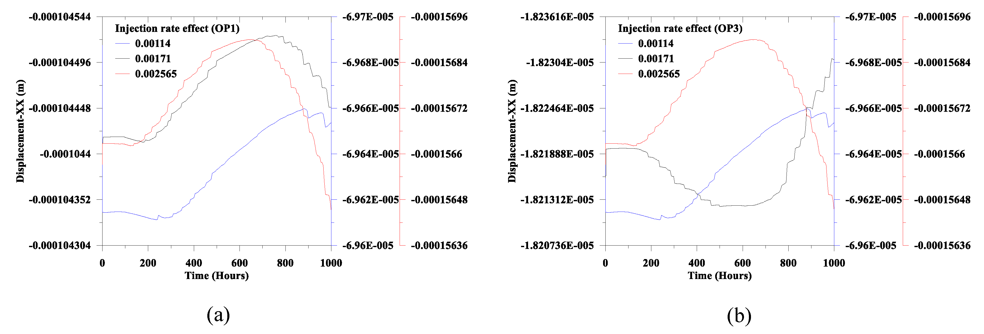
In this section, we present the injection rate effect of primary variables in the coupled hydro-mechanical solutions. We consider three different injection rates. In addition, for this investigation, we present results for two observation points. They are close to the injection face (OP1) and a point in the cement’s fracture (OP3) (see also Figure 10b). Additionally, for this study, we use the monolithic coupling. In addition, we did not use the mass lumping and the upwinding so that with respect to the injection rate, we may obtain the maximum values of primary variables in the coupled solution. The objective of such an investigation is to find the effect of the injection rate on the hydro-mechanical behavior of compromised well. It is worth mentioning that to store CO2 in a storage reservoir; it is desirable to calculate the CO2 injection rate so that the stress state does not exceed the failure criterion, which can be obtained from the laboratory experiments. In addition, it is to note that herein, we use finite element model parameters for the compromised well as an arbitrary value. Therefore, to present a comparison of the experimental results are beyond the scope of this paper.
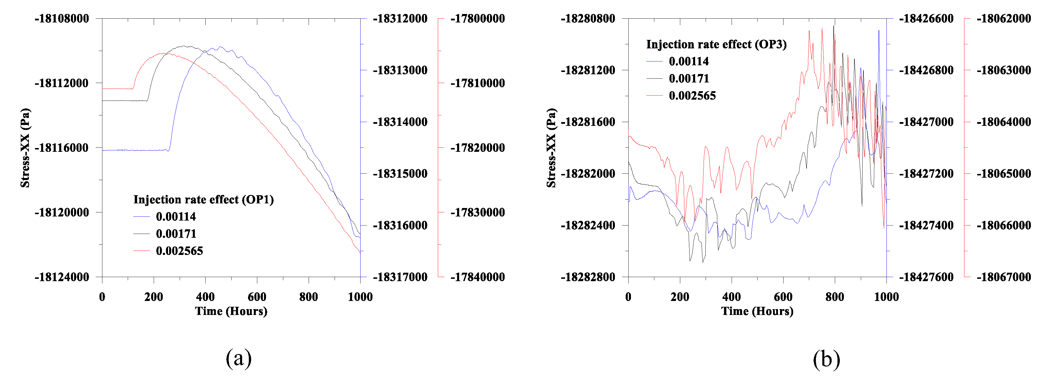
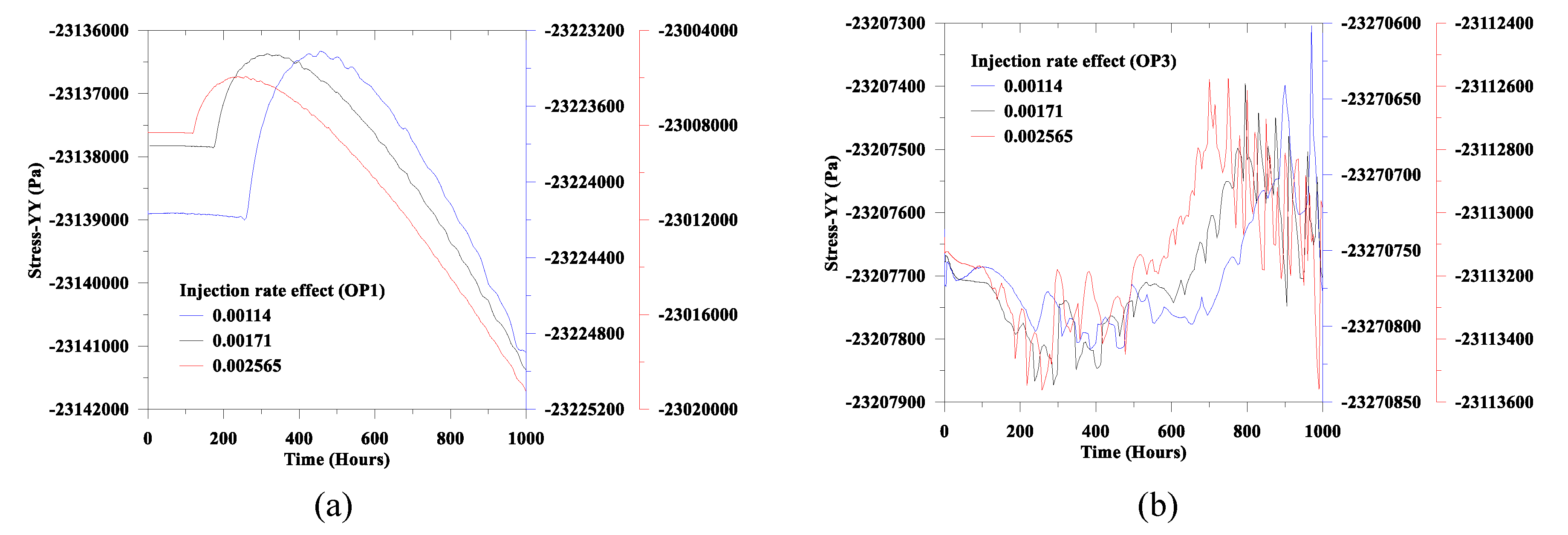
From Figure 15a, we find that with the increase of time, the displacement component along the x-axis gradually increases. Then, after attaining the peak, the displacement component starts to decline. In addition, from Figure 16a and Figure 17a, we notice that with the increase of the injection rate, time for the phase transition of the stress component along the x-axis, and the y-axis decreases. In these two Figures, the straight-line portion on the left side represents the phase transition of the stress state. We also notice from Figure 16a and Figure 17a that after the transition of stress state, the stress components start to decline, which is inversely proportional to the injection rate. Additionally, we find that the stress state starts to increase with the injection rate after the maximum decrease of the stress following the transition. The possible reason to develop such a transformation is relevant to the stress shock during CO2 injection, which results from dropping the stress state. Moreover, the required time to change the stress state from the lowest values to the increase of stress may be related to the energy dissipation of the porous media. It is worth mentioning that during and after the CO2 injection, the dilative and contractive nature of the stress components are crucial for the stability of the compromised well. If such a stress reversal exceeds the limiting stress condition of geomaterial, it may result in a failure state.
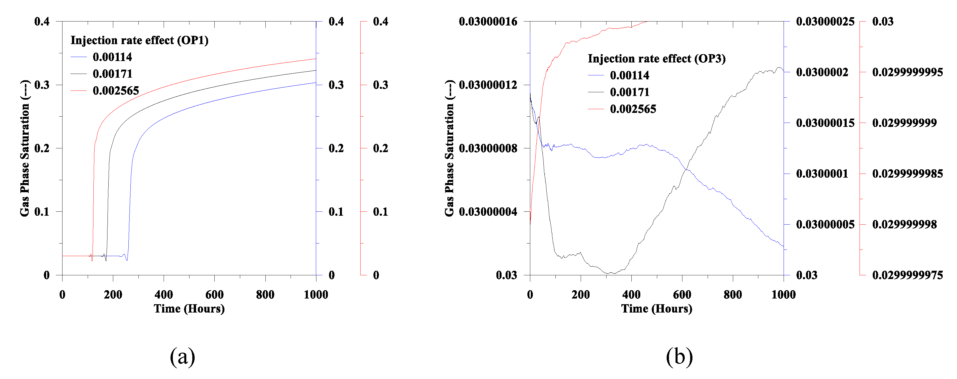
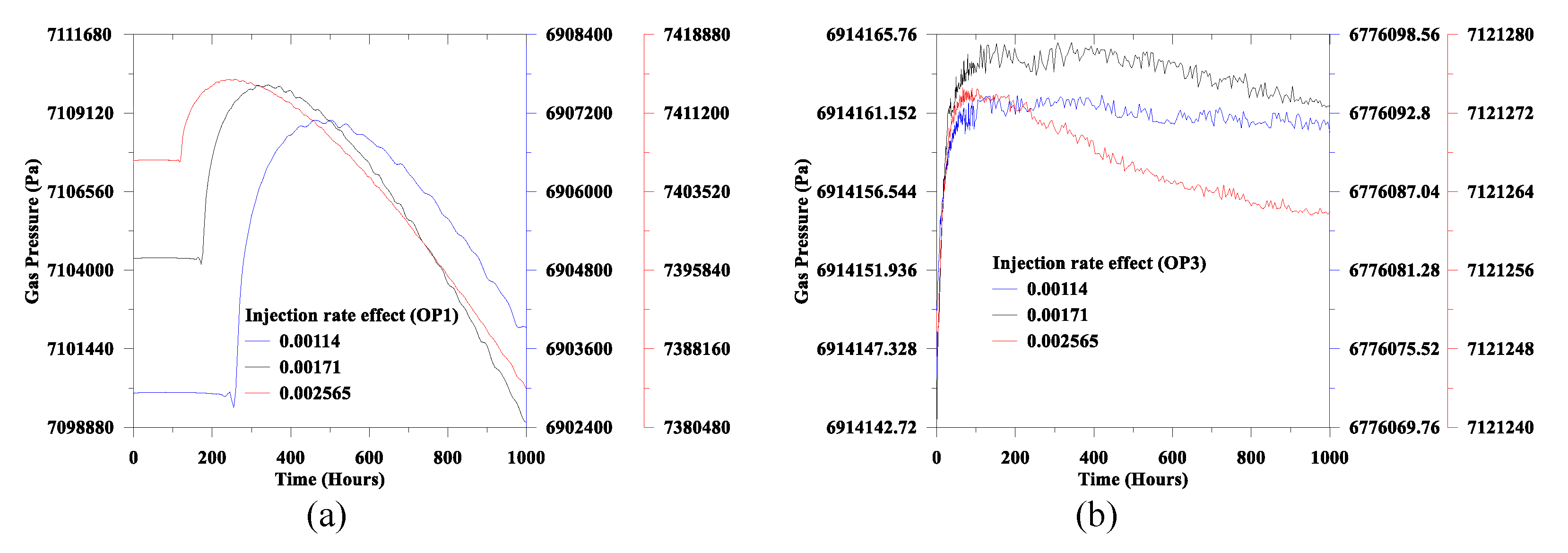
Additionally, from Figure 18a and Figure 19a, the gas phase saturation and the gas pressure follow a similar trend to the stress component, as discussed earlier. Moreover, along the fracture, we notice an oscillation in the stress component and the gas pressure. In this regard, it is noteworthy that considering the parallel plate concept for fracture and ignoring the fracture propagation; it is assuming that the fluid phases are flowing through a thin conduit. From the experimental and numerical evidence, in a thin conduit, development of these types of oscillations are also common (see also, Islam et al. [47]).
7. Conclusions
In this paper, we present a coupled multi-phase flow and deformation flow model. In addition, assuming the gas phase is immobile, we obtained the coupled Richards flow. Then, we compared coupled two-phase flow, Richards flow with Liakopoulos experiments. We found good agreement with the numerical results with an experimental benchmark solution, demonstrating the efficacy of both coupled solutions. It is worth mentioning that even though both solutions provided identical results, but when both fluids (e.g., brine and CO2) are mobile, like, CO2 injection, the Richards solutions may not be appropriate for its assumptions.
Additionally, in the two-phase flow solutions, we present the effect of primary variables selection, considering two sets of primary variables: capillary pressure and the gas pressure (PP scheme) and liquid pressure and the gas saturation (PS scheme). For the homogeneous medium, the effect of fluid primary variables scheme is not significant, but for heterogeneous media (e.g., compromised well scenario), the selection of fluids’ primary variables significantly impacts the accuracy of results. We compared results from both schemes using the Kueper and Frind benchmark experiments. We found that before the displacing fluid plume reaches different interface layer, both algorithms provide similar results, due to homogeneity. However, when the displacing fluid plume reaches the interface layer of two different materials, the PS scheme failed to capture the experimental results. In contrast, the PP scheme results showed good agreement with the benchmark experiments. Based on this comparison, we note that for the heterogeneous media, careful consideration of the fluid phase primary variable scheme is critical to ensure accuracy of the predicted system behavior.
In heterogeneous medium, convergence in numerical modeling proved challenging. Introducing mass lumping (wherein the mass matrix is diagonalized) and the upwinding (wherein the second-order partial differential equation is replaced with the first-order solution along the flow direction) in the numerical solution scheme was used to address this problem. From the benchmark comparison of the Kueper and Frind experiments, we found that with the mass lumping and upwinding, the simulation time is significantly reduced as compared to simulations without applying those approaches. In short-term simulation, both techniques (with and without the mass lumping and the upwinding) provided an identical result. This suggests that these approaches can be used in longer-term simulations of the benchmark problem without impacting fidelity, but this finding must also be tested on the more-complex compromised well scenario. We also presented an optimization method to reduce the computational time for the Kueper and Frind experiments. We found that the auto time-stepping algorithms required between four and five times more computational time. These types of optimization methods are essential to reduce the computational time for the long-term prediction in the compromised legacy well simulation.
A geologic carbon storage compromised plugged legacy well scenario was developed consisting of a geologic CO2 storage reservoir, cement sheath between steel casing and host rock, and a horizontal fracture. Numerical simulation results of this compromised well scenario for the monolithic coupling, with and without the mass lumping and the upwinding techniques. Considering this heterogeneous problem, using upwinding alone in the sequential coupling did not address convergence issues. We also found that using both mass lumping and the upwinding for the long-term prediction yielded results that were significantly lower than the monolithic coupling case. In contrast, to the Kueper and Frind benchmark experiment where the convergence was achieved, computational time was reduced, and fidelity was maintained, the mass lumping and the upwinding techniques failed to work on the long-term compromised legacy well scenario, and should be avoided on problems of this complexity.
Lastly, we found that a safe CO2 injection rate is needed to avoid the mechanical failure condition in the compromised well. Considering three different types of injection rates we found that long-term predictions showed gradually increasing radial displacement of the solid phase. After reaching peak radial displacement energy dissipated and the displacement magnitude began to decrease. At higher injection rate, stress shock resulted in reduction to the stress component (inversely proportional to the injection rate), with subsequent increase in stress component. In addition, for the initial phase of the CO2 injection due to the developed extension at the well surface, the stress component starts to decline. Then, in the domain, the fluid phase displacement results to increase the fluid pressure progressively and the stress component also increases. These types of dilative and contractive geo-mechanical behaviors are critical for the compromised legacy well. The gradual increase of the CO2 pressure in the storage reservoir resulted in changing the hydro-mechanical behavior of the system. It is important that CO2 injection operations should be controlled such that maximum magnitude of the stress component should be lower than the failure condition to ensure safe CO2 injection.
Author Contributions
Conceptualization, all authors.; methodology, all authors.; software, M.I.; validation, M.I. formal analysis, M.I.; investigation, all authors; data curation, M.I.; writing—original draft preparation, M.I.; writing—review and editing, all authors; visualization, M.I.; supervision, R.D. and N.H.; project administration, R.D.; funding acquisition, R.D. All authors have read and agreed to the published version of the manuscript.
Funding
This research received no external funding.
Acknowledgments
This project was supported by appointment to the Science Education Programs at the National Energy Technology Laboratory (NETL) under the National Risk Assessment Partnership (NRAP), administered by the Oak Ridge Associated Universities (ORAU) through the U.S. Department of Energy (DOE).
Conflicts of Interest
The authors declare no conflict of interest.
Appendix A. Constitutive Relations
From the volume balance relation, we obtain a relation between the liquid phase saturation () and the gas phase saturation () as (see Bear and Bachmat [29])
In addition, we assume that the porous medium consists of two fluids (liquid and gas). We obtain fluids’ pressure relations in terms of the capillary pressure () as (see Bear and Bachmat [29])
In Equation (1), the constitutive relations of and are written as, respectively (see Lewis and Schrefler [17])
where is the effective Cauchy stress tensor. , , and are stress tensor of solid, liquid, and the gas phase. , , and are density of each phase. is the porosity. , , and are the reference density of each phase.
Substituting Equations (A3) and (A4) into Equation (1), we find
Assuming the solid phase is inert and substituting Equation (A4) into Equation (2) and expanding for the solid and the fluids, we obtain
where and are the solid phase velocity and the absolute velocity of the fluid phases , respectively. For the two-phases fluids flow, including the relative permeability, we find the Darcy’s equation as (see also, Helmig [18]; Bear and Bachmat [29])
where is known as the phase mobility. and are the intrinsic permeability and the relative permeability, respectively. is the viscosity of the fluids and can be written as
In Equation (A7), using the chain rule, can be expanded as
We assume that fluids’ phases densities are the function of pressure, only. In addition, we consider the isothermal condition and ignore the geochemistry. Moreover, we ignore components of the fluids phase (e.g., vapor). Thereby, we obtain term in Equation (A10) as
where is the initial density at the initial time when initial liquid pressure is . is the compressibility coefficient. M, R, and T are the molar mass, the universal gas constant and the isothermal state temperature. In addition, in Equation (A10) can be expanded with respect to the fluids phase primary variables.
In Equation (A6), is written as (Bear and Bachmat [29])
where represents the time derivative. is the volumetric strain.
Satisfying the small deformation theory and the symmetry condition, we find
Combining Equations (A6)–(A16), then simplifying (see also Islam et al. [47])
Depending on the primary variables of the fluid phases, Equations (A5) and (A17) can be reformulated using Equations (A1) and (A2) for the PP scheme (see Equations (3)–(5)) and the PS scheme (see Equations (6)–(8)). Again, in Equations (A5) and (A17), assuming the gas phase is immobile, we also find the coupled Richards solutions. The number of equations and variables for (i) two-phase fluids, (ii) coupled two-phase fluids and deformation, and (iii) coupled Richards flow and deformation flow are 12 (see Bear and Bachmat [29]), 34 (Table A1 and Table A2), and 25, respectively.
In this paper, we assume that the medium is the isotropic poroelastic material. The elastic strain is given by (see Lubliner [48])
where is the Young’s modulus, and is the Poisson’s ratio, is the effective stress. is the Kronecker delta ().
Additionally, in Equation (A17), to model the transition between the wetting phase (liquid) and the non-wetting phase (gas) saturation, we obtain the capillary pressure and the relative permeability relationship using the Brooks and Corey [25] model as follows
where , , and are the effective saturation, the residual liquid saturation, and the residual gas saturation, respectively. and are the relative permeability of the liquid and the gas, respectively. is the Brooks–Corey parameter. is the air entry pressure. It is worth noting that Lenhard et al. [49] presented an empirical relation to transfer model between the Brooks and Corey [25] model and the van Genuchten [50] model.

Table A1.
List of equations.
| Equation Name | References | Number of Equations |
|---|---|---|
| Linear momentum equation for solid | Equation (1) | 3 |
| Linear momentum equation for liquid | 3 | |
| Linear momentum equation for gas | 3 | |
| Mass conservation equation for solid | Equation (2) | 1 |
| Mass conservation equation for liquid | 1 | |
| Mass conservation equation for gas | 1 | |
| Stress–strain equation | Equation (A18) | 6 |
| Strain displacement equation | Equation (A16) | 6 |
| Darcy’s law for liquid | Equation (A8) | 3 |
| Darcy’s law for gas | 3 | |
| Capillary pressure and saturation relation | Equation (A22) | 1 |
| Density equation for solid | Equation (A4) | 1 |
| Density equation for liquid | Equation (A4) | 1 |
| Density equation for gas | Equation (A4) | 1 |
| Total | 34 |
Table A2.
List of unknown variables.
| Variables | Total | ||||||||||||||
|---|---|---|---|---|---|---|---|---|---|---|---|---|---|---|---|
| Number of unknowns | 6 | 6 | 3 | 3 | 3 | 1 | 1 | 1 | 1 | 1 | 1 | 3 | 3 | 1 | 34 |
References
- Volk, T. CO2 Rising: The World’s Greatest Environmental Challenge; MIT Press: Cambridge, MA, USA, 2008. [Google Scholar]
- Nordbotten, J.M.; Celia, M.A. Geological Storage of CO2 Modeling Approaches for Large-Scale Simulation; John Wiley and Sons: Hoboken, NJ, USA, 2012. [Google Scholar]
- Bachu, S. Sequestration of CO2 in geological media: criteria and approach for site selection in response to climate change. Energy Convers. Manag. 2000, 41, 953–970. [Google Scholar] [CrossRef]
- Choi, Y.-S.; Young, D.; Nesic, S.; Gray, L.G.S. Wellbore integrity and corrosion of carbon steel in CO2 geologic storage environments: A literature review. Int. J. Greenh. Gas Control 2013, 16, S70–S77. [Google Scholar] [CrossRef]
- Pawar, R.J.; Bromhal, G.S.; Carey, J.W.; Foxall, W.; Korre, A.; Ringrose, P.S.; Tucker, O.; Watson, M.N.; White, J.A. Recent advances in risk assessment and risk management of geologic CO2 storage. Int. J. Greenh. Gas Control 2015, 40, 292–311. [Google Scholar] [CrossRef] [Green Version]
- Gomez, S.P.; Sobolik, S.R.; Matteo, E.N.; Reda Taha, M.; Stormont, J.C. Investigation of wellbore microannulus permeability under stress via experimental wellbore mock-up and finite element modeling. Comput. Geotech. 2017, 83, 168–177. [Google Scholar] [CrossRef] [Green Version]
- Bois, A.-P.; Garnier, A.; Rodot, F.; Sain-Marc, J.; Aimard, N. How To Prevent Loss of Zonal Isolation Through a Comprehensive Analysis of Microannulus Formation. SPE Drill. Completion 2011, 26, 13–31. [Google Scholar] [CrossRef]
- Gasda, S.E.; Bachu, S.; Celia, M.A. Spatial characterization of the location of potentially leaky wells penetrating a deep saline aquifer in a mature sedimentary basin. Environ. Geol. 2004, 46, 707–720. [Google Scholar] [CrossRef]
- Celia, M.A.; Bachu, S.; Nordbotten, J.M.; Gasda, S.E.; Dahle, H.K. Quantitative estimation of CO2 leakage from geological storage: Analytical models, numerical models, and data needs. In Greenhouse Gas Control Technologies 7; Rubin, E.S., Keith, D.W., Gilboy, C.F., Wilson, M., Morris, T., Gale, J., Thambimuthu, K., Eds.; Elsevier Science Ltd.: Oxford, UK, 2005; pp. 663–671. [Google Scholar] [CrossRef]
- Wang, W.; Taleghani, A.D. Three-dimensional analysis of cement sheath integrity around Wellbores. J. Pet. Sci. Eng. 2014, 121, 38–51. [Google Scholar] [CrossRef]
- United States Environmental Protection Agency. Determination of the Mechanical Integrity of Injection Wells: United States Environmental Protection Agency, Region 5: Underground Injection Control (UIC) Branch, Regional Guidance #5; US Environmental Protection Agency: Washington, DC, USA, 2008.
- Cavanagh, P.H.; Johnson, C.R.; le Roy-Delage, S.; DeBruijn, G.G.; Cooper, I.; Guillot, D.J.; Bulte, H.; Dargaud, B. Self-Healing Cement—Novel Technology to Achieve Leak-Free Wells. In Proceedings of the SPE/IADC Drilling Conference, Amsterdam, The Netherlands, 20–22 February 2007; p. 13. [Google Scholar]
- Dusseault, M.; Jackson, R. Seepage pathway assessment for natural gas to shallow groundwater during well stimulation, in production, and after abandonment. Environ. Geosci. 2014, 21, 107–126. [Google Scholar] [CrossRef]
- Rutqvist, J. The Geomechanics of CO2 Storage in Deep Sedimentary Formations. Geotech. Geol. Eng. 2012, 30, 525–551. [Google Scholar] [CrossRef] [Green Version]
- Chen, F.; Wiese, B.; Zhou, Q.; Kowalsky, M.B.; Norden, B.; Kempka, T.; Birkholzer, J.T. Numerical modeling of the pumping tests at the Ketzin pilot site for CO2 injection: Model calibration and heterogeneity effects. Int. J. Greenh. Gas Control 2014, 22, 200–212. [Google Scholar] [CrossRef]
- Liakopoulos, A.C. Retention and distribution of moisture in soils after infiltration has ceased. Hydrol. Sci. J. 1965, 10, 58–69. [Google Scholar] [CrossRef]
- Lewis, R.W.; Schrefler, B.A. The Finite Element Method in the Static and Dynamic Deformation and Consolidation of Porous Media, 2nd ed.; John Wiley & Sons: Hoboken, NJ, USA, 1998. [Google Scholar]
- Helmig, R. Multiphase Flow and Transport Processes in the Subsurface: A Contribution to the Modeling of Hydrosystems; Springer: Berlin/Heidelberg, Germany, 1997. [Google Scholar]
- Kueper, B.H.; Frind, E.O. Two-phase flow in heterogeneous porous media: 1. Model development. Water Resour. Res. 1991, 27, 1049–1057. [Google Scholar] [CrossRef]
- Binning, P.; Celia, M.A. Practical implementation of the fractional flow approach to multi-phase flow simulation. Adv. Water Resour. 1999, 22, 461–478. [Google Scholar] [CrossRef]
- Kolditz, O.; Gorke, U.-J.; Shao, H.; Wang, W. Thermo-Hydro-Mechanical-Chemical Processes in Fractured Porous Media: Benchmarks and Examples; Springer: Berlin/Heidelberg, Germany, 2012. [Google Scholar]
- Zienkiewicz, O.C.; Taylor, R.L.; Zhu, J.Z. The Finite Element Method: Its Basis and Fundamentals, 6th ed.; Elsevier: New York, NY, USA, 2005. [Google Scholar]
- Chen, Z.; Huan, G.; Ma, Y. Computational Methods for Multiphase Flows in Porous Media; Society for Industrial and Applied Mathematics: Philadelphia, PA, USA, 2006. [Google Scholar]
- Bacon, D.; Zheng, L.; Yonkofski, C.; Demirkanli, I.; Rose, K.; Zhou, Q.; Yang, Y.-M. National Risk Assessment Partnership—Application of Risk Assessment Tools and Methodologies to Synthetic and Field Data (PNNL-SA-137185); Department of Energy, National Energy Technology Laboratory: Albany, OR, USA, 2018.
- Brooks, R.H.; Corey, A.T. Hydraulic Properties of Porous Media, Hydrology Papers 3; Colorado State University: Fort Collins, CO, USA, 1964; p. 27. [Google Scholar]
- Coussy, O. Poromechanics; John Wiley and Sons: Hoboken, NJ, USA, 2004. [Google Scholar]
- Kolditz, O.; Bauer, S.; Bilke, L.; Böttcher, N.; Delfs, J.O.; Fischer, T.; Görke, U.J.; Kalbacher, T.; Kosakowski, G.; McDermott, C.I.; et al. OpenGeoSys: an open-source initiative for numerical simulation of thermo-hydro-mechanical/chemical (THM/C) processes in porous media. Environ. Earth Sci. 2012, 67, 589–599. [Google Scholar] [CrossRef]
- Geuzaine, C.; Remacle, J.-F. Gmsh: A 3-D finite element mesh generator with built-in pre- and post-processing facilities. Int. J. Numer. Methods Eng. 2009, 79, 1309–1331. [Google Scholar] [CrossRef]
- Bear, J.; Bachmat, Y. Introduction to Modeling of Transport Phenomena in Porous Media; Kluwer Academic Publishers: London, UK, 1990; Volume 4. [Google Scholar]
- De Boer, R. Trends in Continuum Mechanics in Porous Media; Springer: Berlin/Heidelberg, Germany, 2005. [Google Scholar]
- Truesdell, C. Rational Thermodynamics, 2nd ed.; Springer: New York, NY, USA, 1984. [Google Scholar]
- Panday, S.; Corapcioglu, M.Y. Reservoir transport equations by compositional approach. Transp. Porous Media 1989, 4, 369–393. [Google Scholar] [CrossRef]
- Aziz, K.; Settari, A. Petroleum Reservoir Simulation; Applied Science Publishers Ltd.: London, UK, 1979. [Google Scholar]
- Peiro, J.; Sherwin, S. Finite difference, finite element and finite volume methods for partial differential equations. Chapter 8.2. In Handbook of Materials Modeling; Yip, S., Ed.; Springer: Berlin/Heidelberg, Germany, 2005; pp. 2415–2446. [Google Scholar]
- Gundersen, E.; Langtangen, H.P. Finite Element Methods for Two-Phase Flow in Heterogeneous Porous Media. Chapter 10. In Numerical Methods and Software Tools in Industrial Mathematics; Daehlen, M., Tveito, A., Eds.; Springer: New York, NY, USA, 1997. [Google Scholar]
- Paniconi, C.; Putti, M. A comparison of Picard and Newton iteration in the numerical solution of multidimensional variably saturated flow problems. Water Resour. Res. 1994, 30, 3357–3374. [Google Scholar] [CrossRef]
- Saad, Y. Iterative Methods for Sparse Linear Systems; The Society for Industrial and Applied Mathematics: Philadelphia, PA, USA, 2003. [Google Scholar]
- Wood, W.L. Practical Time-Stepping Schemes; Oxford University Press: Oxford, UK, 1990. [Google Scholar]
- Lewis, R.W.; Roberts, P.M. The Finite element method in porous media flow. In Fundamentals of Transport Phenomena in Porous Media; Bear, J., Corapcioglu, M.Y., Eds.; Martinus Nijhoff Publishers: Boston, MA, USA, 1984. [Google Scholar]
- Terzaghi, K. Theoretical Soil Mechanics; John Wiley and Sons: New York, NY, USA, 1943. [Google Scholar]
- Murad, M.A.; Loula, A.F.D. Improved accuracy in finite element analysis of Biot’s consolidation problem. Comput. Methods Appl. Mech. Eng. 1992, 95, 359–382. [Google Scholar] [CrossRef]
- Liakopoulos, A.C. Transient Flow through Unsaturated Porous Media; University of California: Los Angeles, CA, USA, 1965. [Google Scholar]
- Richards, L.A. Capillary conduction of liquids through porous mediums. J. Appl. Phys. 1931, 1, 318–333. [Google Scholar] [CrossRef]
- Schrefler, B.A.; Scotta, R. A fully coupled dynamic model for two-phase fluid flow in deformable porous media. Comput. Methods Appl. Mech. Eng. 2001, 190, 3223–3246. [Google Scholar] [CrossRef]
- Ravi, K.; Bosma, M.; Gastebled, O. Safe and Economic Gas Wells through Cement Design for Life of the Well. In Proceedings of the SPE Gas Technology Symposium, Calgary, AB, Canada, 30 April–2 May 2002; p. 15. [Google Scholar]
- NIST-WebBook. NIST Chemistry WebBook; NIST Standard Reference Database; National Institute of Standards and Technology: Gaithersburg, MD, USA, 2019.
- Islam, M.N.; Bunger, A.P.; Huerta, N.; Dilmore, R. Bentonite Extrusion into Near-Borehole Fracture. Geosciences 2019, 9, 495. [Google Scholar] [CrossRef] [Green Version]
- Lubliner, J. Plasticity Theory; Dover Publications: New York, NY, USA, 1990. [Google Scholar]
- Lenhard, R.J.; Parker, J.C.; Mishra, S. On the Correspondence between Brooks-Corey and van Genuchten Models. J. Irrig. Drain. Eng. 1989, 115, 744–751. [Google Scholar] [CrossRef]
- Van Genuchten, M.T. A closed form equation for predicting the hydrauclic conductivity of unsaturated soils. Soil Sci. Soc. Am. J. 1980, 44, 892–898. [Google Scholar] [CrossRef] [Green Version]
Figure 1.
Schematic section of a compromised well: (a) Geologic block [24] and (b) possible fluid leakage path [8].

Figure 2.
Representative averaging volume of a three-phase system (see also Bear and Bachmat [29]; Lewis and Schrefler [17]).

Figure 3.
Initial and boundary condition of Terzaghi’s 1D consolidation solution.

Figure 4.
Comparison between the Terzaghi’s 1D consolidation analytical solution and finite element results at the bottom.
Figure 4.
Comparison between the Terzaghi’s 1D consolidation analytical solution and finite element results at the bottom.

Figure 5.
Liakopoulos test arrangement (a) , and (b) (Note: not in scale).

Figure 6.
Finite element results and Liakopoulos experiments: (a) water pressure, (b) outflow rate, (c) water saturation, and (d) vertical displacement.
Figure 6.
Finite element results and Liakopoulos experiments: (a) water pressure, (b) outflow rate, (c) water saturation, and (d) vertical displacement.

Figure 7.
Configuration of heterogeneous sand lenses in parallel plate cell (see Kueper and Frind [19]).
Figure 7.
Configuration of heterogeneous sand lenses in parallel plate cell (see Kueper and Frind [19]).

Figure 8.
Comparison of observed (redrawn) and predicted tetrachloroethylene distribution in terms of the liquid at 34 s (a–c) and 313 s (d–f).
Figure 8.
Comparison of observed (redrawn) and predicted tetrachloroethylene distribution in terms of the liquid at 34 s (a–c) and 313 s (d–f).

Figure 9.
Comparison of predicted tetrachloroethylene distribution in terms of the liquid at 313 Sec: (a–c) with the mass lumping and the upwinding and (d–f) without the mass lumping and the upwinding.
Figure 9.
Comparison of predicted tetrachloroethylene distribution in terms of the liquid at 313 Sec: (a–c) with the mass lumping and the upwinding and (d–f) without the mass lumping and the upwinding.

Figure 10.
(a) Schematic diagram of the cross-section of the compromised well and (b) schematic dimensions of the cross-section and locations of observation points (see also Ravi et al. [45]).
Figure 10.
(a) Schematic diagram of the cross-section of the compromised well and (b) schematic dimensions of the cross-section and locations of observation points (see also Ravi et al. [45]).

Figure 11.
Comparisons of the displacement along the X-axis: (a) the monolithic coupling and the sequential coupling and (b) with and without the mass lumping and the upwinding.
Figure 11.
Comparisons of the displacement along the X-axis: (a) the monolithic coupling and the sequential coupling and (b) with and without the mass lumping and the upwinding.

Figure 12.
Comparisons of the stress along the X-axis: (a) the monolithic coupling and the sequential coupling and (b) with and without the mass lumping and the upwinding.
Figure 12.
Comparisons of the stress along the X-axis: (a) the monolithic coupling and the sequential coupling and (b) with and without the mass lumping and the upwinding.

Figure 13.
Comparisons of the gas phase saturation: (a) the monolithic coupling and the sequential coupling and (b) with and without the mass lumping and the upwinding.
Figure 13.
Comparisons of the gas phase saturation: (a) the monolithic coupling and the sequential coupling and (b) with and without the mass lumping and the upwinding.

Figure 14.
Comparisons of the gas phase velocity: (a) the monolithic coupling and the sequential coupling and (b) with and without the mass lumping and the upwinding.
Figure 14.
Comparisons of the gas phase velocity: (a) the monolithic coupling and the sequential coupling and (b) with and without the mass lumping and the upwinding.

Figure 15.
Injection rate effect on the x-axis displacement: (a) OP1 and (b) OP3.

Figure 16.
Injection rate effect on the x-axis stress: (a) OP1 and (b) OP3.

Figure 17.
Injection rate effect on the y-axis stress: (a) OP1 and (b) OP3.

Figure 18.
Injection rate effect on the gas saturation: (a) OP1 and (b) OP3.

Figure 19.
Injection rate effect on the gas pressure: (a) OP1 and (b) OP3.

Table 1.
Physical parameters for 1D Terzaghi’s consolidation.
| Parameters | Symbol | Unit | Value |
|---|---|---|---|
| Young’s Modulus | E | Pa | 3.0 × 10⁴ |
| Poisson’s ratio | ν | --- | 0.20 |
| Porosity | φ | --- | 0.50 |
| Permeability | k | m2 | 1.0 × 10⁻¹⁰ |
| Liquid density | kg/m3 | 1000 | |
| Liquid viscosity | Pa-s | 1.0 × 10⁻³ |
Table 2.
Physical parameters for the Liakopoulos test.
| Parameters | Symbol | Unit | Value |
|---|---|---|---|
| Young’s Modulus * | E | Pa | 1.3 × 10⁶ |
| Poisson’s ratio * | ν | --- | 0.40 |
| Porosity | φ | --- | 0.2975 |
| Solid’s density | kg/m3 | 2000 | |
| Permeability | K | m2 | 4.5 × 10⁻¹³ |
| Liquid density | kg/m3 | 1000 | |
| Liquid viscosity | Pa-s | 1.0 × 10⁻³ | |
| Air density | kg/m3 | Ideal Gas Law’s | |
| Air viscosity | Pa-s | 1.8 × 10⁻⁵ | |
| Atmospheric reference pressure | Pa | 0 | |
| Capillary pressure § | Pa | ||
| Liquid phase relative permeability § | --- | ||
| Gas phase relative permeability ‡ | --- |
Table 3.
Fluid properties.
| Fluid Properties | Symbol | Unit | Water | Tetrachloroethylene |
|---|---|---|---|---|
| Density | kg/m3 | 1 × 10³ | 1.63 × 10³ | |
| Viscosity | Pa-s | 1 × 10⁻³ | 0.90 × 10⁻³ |
Table 4.
Brooks–Corey model parameter for heterogeneous sand lenses in parallel plate cell.
| Sand | (-) | S | k (m2) | n (-) | |
|---|---|---|---|---|---|
| #16 Silica | 369.73 | 3.86 | 0.078 | 5.04 × 10⁻¹⁰ | 0.40 |
| #25 Ottawa | 434.45 | 3.51 | 0.069 | 2.05 × 10⁻¹⁰ | 0.39 |
| #50 Ottawa | 1323.95 | 2.49 | 0.098 | 5.26 × 10⁻¹¹ | 0.39 |
| #70 Silica | 3246.15 | 3.30 | 0.189 | 8.19 × 10⁻¹² | 0.41 |
Table 5.
Computational time with and without the mass lumping and the upwinding.
| Time Step | Computational Time (Hours) for the PP Scheme | |
|---|---|---|
| With the Mass Lumping and the Upwinding | Without the Mass Lumping and the Upwinding | |
| Auto Time Step | 27.06 | 34.70 |
| 15.41 | 17.03 | |
| 7.14 | 8.04 | |
| 5.76 | Convergence problem | |
Note: Computational time in the HP Z840 Workstation (Xeon (R) 2.60 GHz Processor and 16 gb memory).
Table 6.
Properties of casing, reservoir, cement, and fracture.
| Section | Properties | Symbol | Unit | Value | |
|---|---|---|---|---|---|
| Casing | Mechanical | Young’s Modulus | Ecasing | Pa | 1.7 × 10¹¹ |
| Poisson’s Ratio | 0.27 | ||||
| Density | kg/m3 | 8000 | |||
| Porosity | ϕcasing | --- | --- | ||
| Flow | Permeability | kcasing | m2 | 1.0 × 10⁻²¹ | |
| Reservoir | Mechanical | Young’s Modulus | Erock | Pa | 2.0 × 10¹¹ |
| Poisson’s Ratio | 0.30 | ||||
| Density | kg/m3 | 2650 | |||
| Porosity | ϕrock | --- | 0.30 | ||
| Flow | Permeability | krock | m2 | 1.0 × 10⁻¹³ | |
| Cement | Mechanical | Young’s Modulus | Ecement | Pa | 8.3 × 10⁹ |
| Poisson’s Ratio | 0.25 | ||||
| Density | kg/m3 | 2000 | |||
| Porosity | ϕcement | --- | 0.132 | ||
| Flow | Permeability | kcement | m2 | 1 × 10⁻²⁰ | |
| Fracture | Mechanical | Young’s Modulus | Efracture | kPa | 2.0 × 10⁸ |
| Poisson’s Ratio | 0.20 | ||||
| Density | kg/m3 | 1600 | |||
| Porosity | ϕfracture | --- | 0.80 | ||
| Flow | Permeability | kfracture | m2 | 3.25 × 10⁻⁸ | |
| Geometry | Thickness | b | Micro-m | 625 | |
Table 7.
Fluid properties (From NIST webbook NIST [46]).
Table 7.
Fluid properties (From NIST webbook NIST [46]).
| FluidProperties | Symbol | Unit | Fluids | |
|---|---|---|---|---|
| Brine | CO2 | |||
| Density | kg/m3 | 1004.6 | 895.39 | |
| Viscosity | Pa-s | 7.3446 × 10⁻⁴ | 9.0285 × 10⁻⁵ | |
Table 8.
Relative permeability and capillary pressure parameters.
| Items | Unit | Symbol | Reservoir | Cement | Fracture | Casing |
|---|---|---|---|---|---|---|
| Values | ||||||
| Residual CO2 saturation | --- | 0.03 | 0.20 | 0.05 | N/A | |
| Maximum CO2 saturation | --- | 0.60 | 0.70 | 0.90 | ||
| Residual brine saturation | --- | 0.40 | 0.30 | 0.10 | ||
| Maximum brine saturation | --- | 0.97 | 0.80 | 0.95 | ||
| Brooks-Corey parameter | --- | λ | 2 | 2 | 2 | |
| Air entry pressure | Pa | 104 | 104 | 104 | ||
Table 9.
Initial stress conditions.
| Input | Values | Unit |
|---|---|---|
| Overburden pressure | −23.40 × 10⁶–25,996.5 × y | Pa |
| Maximum horizontal stress | −18.72 × 10⁶–20,797.2 × y | Pa |
| Minimum horizontal stress | −18.72 × 10⁶–20,797.2 × y | Pa |
Publisher’s Note: MDPI stays neutral with regard to jurisdictional claims in published maps and institutional affiliations. |
© 2020 by the authors. Licensee MDPI, Basel, Switzerland. This article is an open access article distributed under the terms and conditions of the Creative Commons Attribution (CC BY) license (http://creativecommons.org/licenses/by/4.0/).
Share and Cite
MDPI and ACS Style
Islam, M.; Huerta, N.; Dilmore, R. Effect of Computational Schemes on Coupled Flow and Geo-Mechanical Modeling of CO2 Leakage through a Compromised Well. Computation 2020, 8, 98. https://0-doi-org.brum.beds.ac.uk/10.3390/computation8040098
AMA Style
Islam M, Huerta N, Dilmore R. Effect of Computational Schemes on Coupled Flow and Geo-Mechanical Modeling of CO2 Leakage through a Compromised Well. Computation. 2020; 8(4):98. https://0-doi-org.brum.beds.ac.uk/10.3390/computation8040098
Chicago/Turabian StyleIslam, Mohammad, Nicolas Huerta, and Robert Dilmore. 2020. "Effect of Computational Schemes on Coupled Flow and Geo-Mechanical Modeling of CO2 Leakage through a Compromised Well" Computation 8, no. 4: 98. https://0-doi-org.brum.beds.ac.uk/10.3390/computation8040098
Note that from the first issue of 2016, this journal uses article numbers instead of page numbers. See further details here.