1. Introduction
1.1. General Context
Electrical distribution networks are responsible for interconnecting transmission and sub-transmission grids with final electricity users living in urban and rural areas through substations, conforming the well-known medium- and low-voltage networks [
1,
2]. The main parameter to analyze these networks is power flow. Thus, the power flow problem constitutes a steady-state study where electrical variables (voltages and currents) are determined for a particular load and generation condition [
3,
4]. The main characteristic of the power flow problem is the conformation of a non-linear system of equations as a result of the presence of products of variables and trigonometric functions, which demands the use of numerical methods to find a solution [
5,
6]. Typically, the power flow problem in electrical distribution grids has been addressed only with single-phase equivalents in the literature [
7]. However, some electrical distribution networks cannot be reduced to single-phase equivalents due to the following characteristics: (i) no transposition in distribution lines, i.e., unbalanced impedances among phases, (ii) unbalanced loads with
- and
Y-connections, (iii) single-phase or two-phase laterals [
8,
9,
10]. Thus, distribution networks must be analyzed directly in their three-phase form in order to capture the actual effect of the imbalances in the electrical variables, including voltages, currents, and powers.
1.2. Motivation
Powerful methodologies are always required for the analysis of electrical grids in planning and operational aspects to estimate (calculate) the electrical variables for particular load conditions or variable load cases considering real-time operation scenarios [
11]. In the case of three-phase grids, the unbalanced nature of the loads and impedances makes it necessary to propose efficient numerical methods in order to deal with the power flow problem by considering single-, two-, and three-phase loads, including
- and
Y-connections [
12]. Due to the importance of developing efficient tools for three-phase networks, this research is motivated by the possibility of improving the upper-triangular power flow method for unbalanced distribution networks with the inclusion of the convergence analysis via the Banach fixed-point theorem, with its main advantage being that it is derivative-free. This is important since this will facilitate its implementation using any programming language with simple operations and without variant matrices, which assists in reducing the required processing times for solving the three-phase power flow problem in unbalanced distribution networks. Additionally, we present the general algorithm to handle single-, two-, and three-phase loads with
- and
Y-connections but without modifying the power flow formulation, as the main advantage of our proposed approach is that it does not depends on the reactance/resistance ratio.
1.3. Literature Review
Multiple power flow methods are proposed in the existing literature for the analysis of radial three-phase distribution networks. Authors in [
13] presented a matrix reformulation of the classical three-phase backward/forward power flow method for balanced grids. Even if this method is classical [
14], the authors demonstrated its convergence using the Banach fixed-point theorem. An improved version for unbalanced three-phase grids that consider loads connected in
- and
Y- has been proposed in [
15] to solve the phase-balancing problem by employing a leader–follower optimization approach. The power flow numerical results were compared with the DigSILENT software (three-phase Newton–Raphson method), demonstrating its effectiveness in calculating power losses. Authors in [
8] proposed a decoupled power flow method using a quasi-symmetric matrix formed as a result of the inductive and resistive effects of the distribution lines. This method works in real domains by separating the real and imaginary parts of the voltages. Numerical results demonstrate its computational efficiency when compared with the classical yet complex backward/forward formulation in different IEEE test feeders. Garces in [
4] proposed a linear formulation for the power flow problem in three-phase grids. This formulation was based on Laurent’s series expansion of the hyperbolic relation among voltage and power balance equations. Numerical results contain errors lower than 3% for different IEEE test feeders when compared with the backward/forward power flow method. Authors in [
16] proposed a holomorphic embedding power flow approach for determining the electrical variables in medium- and low-voltage three-phase grids. Numerical results demonstrated the efficiency of this approach when compared with the classical three-phase Newton–Raphson approach. In Sereeter, [
17], extended versions of the classical Newton–Raphson power flow method have been compared with the backward/forward load flow approach. The algorithms’ convergence for different loading conditions, resistance/reactance ratios, and load models was studied by performing numerical experiments on balanced and unbalanced distribution grids. Authors in [
18] presented an iterative methodology for the power flow solution in three-phase distribution networks based on decoupled circuit equivalents in the complex domain. Numerical comparisons with classical tools (such as Newton–Raphson in specialized power system software) demonstrated its effectiveness in large-scale distribution grids. Marini et al. [
19] proposed a graph-based power flow method for radial and meshed distribution networks using an upper-triangular formulation. This paper’s main contribution is to the three-phase modeling of regulators, transformers, and induction machines, among others. Numerical results demonstrate the computational efficiency of the proposed power flow method for different reactance/resistance ratios. Authors of [
20] presented a three-phase power flow approach for islanded microgrids that is based on the Newton–Raphson current injection method in order to deal with the lack of a slack node. The proposed algorithm selects system frequency and voltage magnitude of the reference bus as additional variables in power-flow formulation. Numerical simulations confirm the efficiency of this method for different reactance/resistance ratios, including the best processing time performance, compared to classical Newton–Raphson methods and specialized tools available in the PSCAD software.
In order to summarize the three-phase power flow approaches reported in the literature,
Table 1 presents some approaches applicable to power distribution grids with unbalanced load conditions.
1.4. Contribution and Scope
This paper introduces a modified version of the upper-triangular-based power flow method originally reported in Marini et al. [
19]. The proposed formulation considers three-phase unbalanced distribution systems with loads connected to
and
Y using a matrix representation. The modified power flow is tested on three different networks with 8, 25, and 37 nodes to demonstrate the algorithm’s accuracy and efficiency. The main advantages of the proposed upper-triangular power flow method are as follows: (i) the possibility of working with single-, two-, and three-phase loads with
- and
Y-connections; (ii) independence in the reactance/resistance relations in the distribution lines; and (iii) the processing time performance when compared with the classical backward/forward power flow method.
The computational performance of the triangular-based power flow is assessed within an optimization problem solved through metaheuristics. In this paper, power flow is evaluated using the classical Chu–Beasley genetic algorithm (CBGA) to solve the phase-balancing problem by employing a leader–follower approach. The leader stage is entrusted with defining the configuration of the phases, while the triangular-based power flow method determines the total power losses for each phase configuration defined in the leader stage. The main contributions of this paper to the current literature are as follows:
The analysis of the upper-triangular-based power flow under different load connections, i.e., - and Y-connections.
A convergence analysis based on the Banach fixed-point theorem for three-phase networks with pure Y load connections.
Application of the proposed upper-triangular three-phase power flow method to solve the phase-balancing problem using a CBGA.
Note that these contributions are concentrated in the general power flow formulation for three-phase distribution networks with unbalanced loads and radial configurations; however, the analysis of convergence is only developed for Y-connected loads due to the possibility of generalizing its recursive formula with diagonal matrices and vectors, which is not possible in the case of -connected loads. In this sense, the study of the convergence for loads could be explored in future research.
1.5. Structure of the Document
The remainder of this research is structured as follows:
Section 2 presents the single-phase formulation of the triangular-based power flow method using a small example to explain the main concepts of the non-derivative power flow formulation.
Section 3 presents the three-phase extension of the triangular-based power flow method with a consideration of different load configurations, i.e.,
Y- and
-connections. Moreover,
Section 4 presents the convergence test using the Banach fixed-point theorem for three-phase loads with solidly grounded
Y-connection.
Section 5 presents the information pertaining to test systems; these test feeders are composed of 8, 25, and 37 nodes.
Section 6 presents the numerical results for the test feeder under different load connections, highlighting comparisons with the classical Newton–Raphson and backward/forward methods. Furthermore, the proposed variable of power flow is tested by employing a CBGA leader–follower optimization structure in order to solve the phase-balancing problem. Finally,
Section 7 presents the main conclusions obtained from this research and discusses the possible areas for future work.
2. Single-Phase Power Flow Formulation
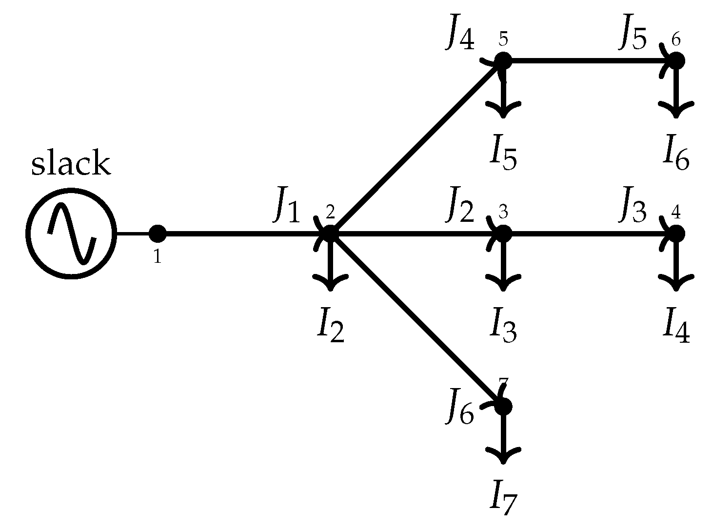
The three-phase power flow problem corresponds to the steady-state formulation of electrical distribution networks with unbalanced loads and different feeder configurations. The idea behind solving this problem is to determine the network state variables, i.e., voltage magnitudes and phase angles. In this paper, we adopted a graph-based representation of electrical distribution grids based on the upper-triangular matrix formulation (it is recommended that the grid is ordered starting from the slack bus). Consider the schematic representation of the 7-node, 6-branch distribution network depicted in
Figure 1 with a single-phase representation.
Note that branch currents
can be expressed as a function of the demanded currents
using the following expression:
Here,
represents the current through the branch
j, and
corresponds to the net injected current at node
i, which can be zero in the case of the step-nodes. A general expression can be compacted into
Here, is the vector that contains all the branch currents in the complex domain (b branches); represents the vector that contains all the demanded currents in the nodes (n) of the network, except in the slack source; represents the upper-triangular matrix.
Consider that
represents the voltages at load buses,
is the voltage at the slack bus, and
is the branch voltage drop. Applying Kirchhoffs’ second law to each trajectory that contains the slack source, i.e.,
, and all the nodes of the network, the following expression is obtained:
This can be expressed in a compact form as:
Here, is a vector that contains all branch voltage drops, represents the vector containing the voltages in demand nodes, and is the voltage at the substation bus. Note that is a vector filled by ones.
Branch voltage drops can be expressed as a function of the branch current after applying Ohm’s law. This is performed by using the primitive impedance matrix
, which has been presented below:
Here, is a complex diagonal matrix containing the branches’ impedance, i.e., .
To obtain a general formula for nodal voltages
and the nodal currents
, (
3) and (
1) are substituted into (
2), producing the following expression:
Note that (
4) can be applied in single-phase distribution grids, where the nodal injected current is calculated as follows:
Here,
is a complex vector that contains all constant power demands, and
stands for the vector’s component conjugate. Now, if (
5) is substituted into (
4), then the following recursive formula is yielded:
Remark 1. Equation (4) relates nodal voltages and injected currents to demand nodes. However, note that constant power demands need to be expressed as current injections. Hence, there is a need to obtain a recursive formula for determining the voltages at demand nodes as a function of constant power demands. 3. Three-Phase Power Flow Formulation
The general formulation of the triangular-based power flow method in three-phase systems needs to consider three possible cases, i.e., power consumption connected in (i) Y-connection, (ii) -connection, and (iii) both load configurations.
3.1. Three-Phase Grid with Demands in Y-Connection
Equation (
4) is transformed into a three-phase expression as follows:
Here, is a vector that contains all the phase voltages ordered per node; is a rectangular matrix filled by identity matrices; is a vector that contains the voltages of the substation node (fixed); represents the three-phase equivalent of the upper-triangular matrix , where each connection (1) is converted into a identity matrix (note that, in case the grid has two-phase or single-phase feeders, the corresponding element in this matrix takes the value zero), and each zero becomes a zeros matrix; is the primitive three-phase impedance matrix, which has a three-diagonal structure (note that three-diagonal matrix form corresponds to a matrix composed of matrices diagonally, with the remainder of the terms being equal to zero); is a vector that contains all the phase currents ordered per node.
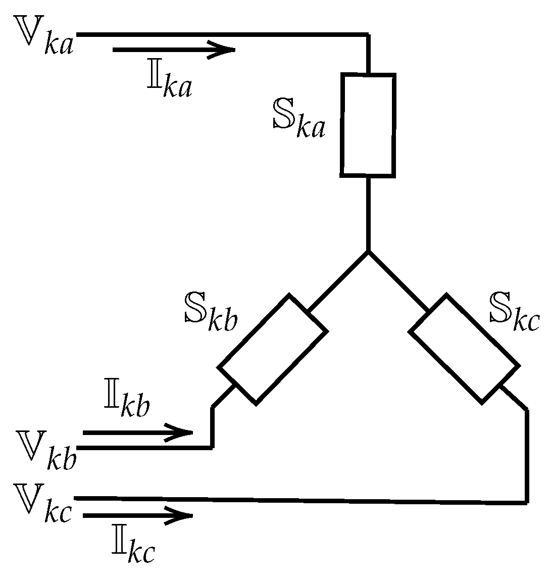
For the purpose of illustration, consider the case where all nodes have constant power loads in the
Y-connection and are solidly grounded. Take the generic
Y-connection for a load at node
k as depicted in
Figure 2.
In the three-phase load with
Y-connection, we assume that the voltage experiencing each load is the phase-to-neutral; with this assumption, each line-current is calculated as follows:
This can be compacted as follows:
Considering the diagonal structure of the three-phase current at node
k, it is possible to generalize the triangular three-phase power flow formulation for three-phase loads connected in
Y as follows:
Remark 2. To solve the upper-triangular three-phase power flow formulation, (9) is added as an iterative counter t, starting from the initial voltages defined as . The recursive formulation of the three-phase power flow problem takes the following form: Note that Equation (10) represents a non-derivative power flow method for three-phase distribution grids with balanced or unbalanced structures. The main advantage of this formulation is its simplicity since the impedance-like matrix (i.e., ) is calculated one time and stored to improve the processing time performance of the power flow solution. 3.2. Three-Phase Grid with Demands in -Connection
To obtain the line currents for a three-phase network with loads connected in
, consider the load diagram presented in
Figure 3 for the
k node.
This can be compacted into the following:
Here, the matrices
and
take the following form:
Remark 3. To solve the problem of the power flow in three-phase network with Δ loads, the following steps of the iterative procedure were developed:
- 1.
Define the test feeder characteristics and calculate the three-phase impedance-like matrix, i.e., ;
- 2.
Define the starting point of the voltages using the substation voltage;
- 3.
Calculate the current for each node k using (9) for the iteration t as follows: - 4.
Calculate all the voltages in the demand nodes using (7) as presented below: - 5.
Determine whether the convergence error has been fulfilled—if yes, the power flow problem is solved; otherwise, update the starting voltage point and return to step 3.
3.3. Three-Phase Grid with Demands in - and Y-Connections
In the case that a three-phase distribution grid has loads connected with
Y and
structures, the calculation of the demanded currents must consider these connections as presented in Equations (
8) and (
11), respectively. Algorithm 1 presents the general implementation of the three-phase triangular power flow for unbalanced distribution networks with loads connected in
Y and
.
| Algorithm 1: Pseudo code for the solution of the three-phase power flow problem in unbalanced distribution networks with Y and loads. |
![Computation 09 00061 i001]() |
3.4. Power Losses Calculation
One of the main objectives of the power solution in single- and three-phase grids is computing the amount of power losses in all the conductors of the network after determining all the voltages in the demand nodes. To perform this task, since we know that
and
represent the final voltages and the final demanded currents reported by the power flow solution, which fulfills the convergence criteria, from Equations (
1) and (
3) in their three-phase forms, we know the following:
When these are combined, the following is produced:
Here, represents the apparent power losses in the network.
4. Convergence Analysis for -Connected Loads
The main advantage of the upper-triangular three-phase power flow formulation is the possibility of ensuring convergence when all the three-phase loads have a
Y-connection. Here, we present the convergence test based on the Banach fixed-point theorem. The convergence analysis presented in this section is based on the convergence test for the successive approximation method used in [
7] for single-phase distribution networks. The convergence test is based on the following assumptions [
27]:
Assumption 1. The total consumption of the active active power in the distribution does not cause a voltage collapse, which implies that the power flow equations can be solved.
Assumption 2. The lower bound for all the voltages is positive, i.e., , which is fulfilled by the grid since regulatory policies have made it mandatory.
Assumption 3. The impedance-like matrix is diagonal dominant, suggesting that is always ensured.
To present the convergence properties of the triangular-based power flow method for three-phase networks with the structure defined in (
10), let us consider the general definition of the Banach fixed-point theorem as follows [
13,
27]:
Lemma 1 (Fixed-point theorem).
The recursive formula defined by Equation (10) is stable and defines a contraction map with the following form: for some that fulfills Assumption 1 and independent at the starting point , such that:Here, defines the solution of the three-phase power flow problem, i.e., a vector that contains all the voltages of the demand nodes. In addition, η corresponds to a real number between .
Proof. Note that the iterative expression that defines the triangular-based power method showed in (
10) can be rewritten as follows:
with
being the set that contains all the demand buses ordered per node and phase.
Owing to the structure of the three-phase power flow problem, it is possible to say that the solution
complies with
, and it defines a unique solution, if and only if
corresponds to a contraction mapping on
.
with
Now, if we consider Assumption 3, relating the nature of the impedance-like matrix, Equation (
17) can be transformed into the following:
Note that, considering the structure of (
18) and taking into account that
defines the equivalence impedance at the node
j (i.e., the Thévenin equivalent impedance), the following relation is met:
Here,
can be ensured since the denominator of (
19) can be interpreted as the lowest short-circuit current, while the numerator denotes the maximum loading current. At the same time, it is known that the maximum loading current is lower than or equal to the lowest short-circuit current for any demand scenario. This characteristic of the
-coefficient allows confirmation of the recursive power flow formula (
10) in order to make sure the three-phase power flow problem is stable and converges to the solution
, which completes the proof. □
5. Test Feeders
To validate the proposed three-phase power flow method, let us consider three test feeders composed of 8, 25, and 37 nodes, which have been reported in [
15] for phase-balancing studies.
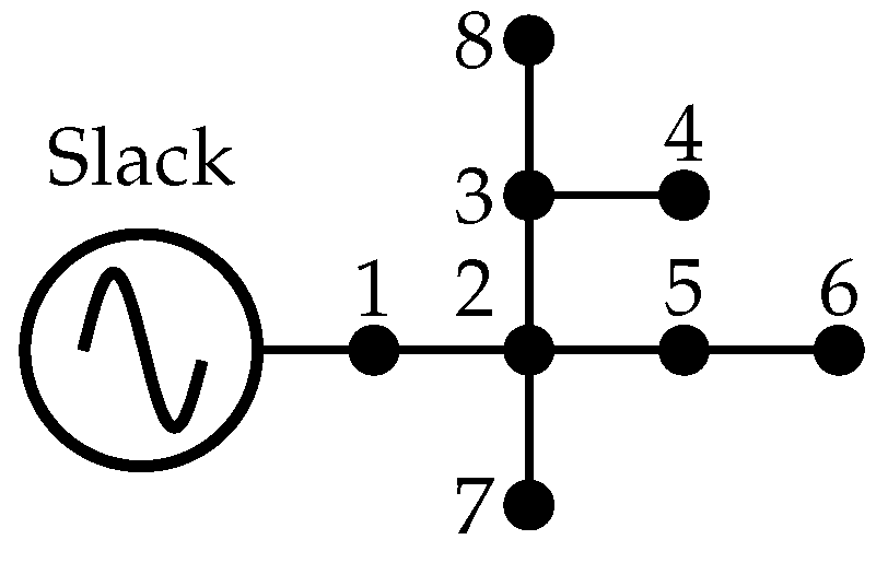
5.1. 8-Bus Test Feeder
The eight-bus test feeder corresponds to a radial distribution network composed of eight nodes and seven lines, where the slack node is located at bus 1 with a line-to-line voltage set at 11 kV. The electrical configuration of this test system is depicted in
Figure 4. In this eight-bus system, the total active and reactive power demands are 1005 kW and 485 kvar for phase
a, 785 kW and 381 kvar for phase
b, and 1696 kW and 821 kvar for phase
c.
The electrical information of the impedances and loads for this test system are presented in
Table 2 and
Table 3, respectively.
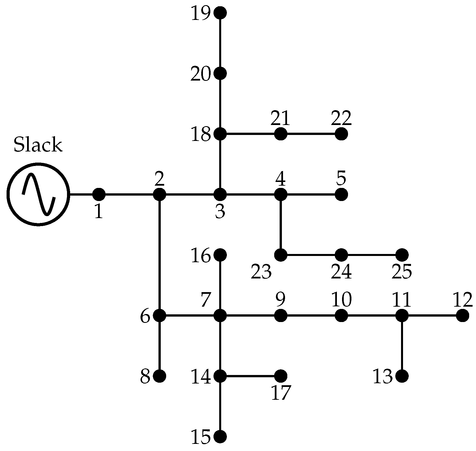
5.2. 25-Bus Test System
The 25-bus system is a radial distribution network with 25 nodes, 24 lines, and 22 constant power loads. The voltage controlled source is located at bus 1, which operates with line-to-line voltage of 4.16 kV.
This is a radial unbalanced distribution system with 25 nodes, 24 lines, and 22 loads. The source is located at node 1, and the nominal voltage is 4.16 kV [
28]. The grid configuration of this test system is presented in
Figure 5. The total loads for phases
a,
b, and
c are 1073 kW and 792 kvar, 1083.3 kW and 801 kvar, and 1083.3 kW and 800 kvar, respectively.
The electrical information of the impedances and loads for this test system are presented in
Table 4 and
Table 5, respectively. This parametric information was taken from [
29].
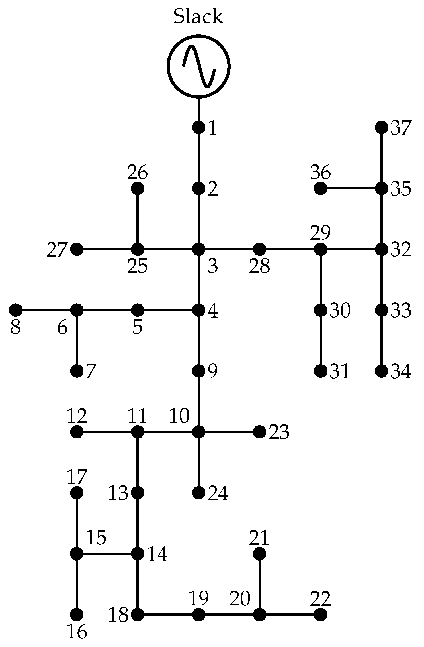
5.3. IEEE 37-Bus System
This test feeder corresponds to a underground system located in the state of California, which is composed of 37 nodes and 36 lines (see its electrical configuration in
Figure 6). The voltage controlled source is connected at node 1 operating with a line-to-line voltage of 4.8 kV. In this system, there are 25 constant power loads, with a total and reactive power consumption in phases
a,
b, and
c of 727 kW and 357 kvar, 639 kW and 314 kvar, and 1091 kW and 530 kvar, respectively. The IEEE 37-bus test system used in this research corresponds to the adaptation proposed in [
15], where the voltage regulator connected between nodes 1 and 2 is replaced by a single three-phase line with a length of 1850 feet, and the transformer located at nodes 10 and 24 is removed, including node 24, as recommended in [
30].
The parametric information for this test feeder is presented in
Table 6 and
Table 7. These data were taken from [
15].
6. Computational Validation
In this section, we present the numerical validation of the proposed non-derivative power flow method for three-phase unbalanced distribution grids with loads connected in
and
Y. The following cases were considered for simulation purposes: (i) evaluation of the power flow assuming that all the loads are connected to
Y, comparing its results with the backward/forward approach reported in [
15] and the classical Newton–Raphson method available in the DigSILENT software; (ii) solution of the three-phase power flow considering all the loads connected in
; (iii) solution of the phase-balancing problem using a leader–follower approach based on the CBGA in the leader stage and the proposed non-derivative triangular-based power flow method in the follower stage.
6.1. Power Flow Solution with Y-Connected Loads
To validate the effectiveness of the non-derivative triangular-based power flow method for solving the power flow problem in three-phase grids, we consider the three test feeders described in the previous section. In addition, the backward/forward and proposed methods are evaluated 10,000 consecutive times each to determine their respective average processing times.
Table 8 presents the numerical values indicating the performance of each power flow method. It is important to mention that the processing time of the Newton–Raphson is not reported as this method is implemented in the DigSILENT software (with a different programming environment than the MATLAB used for the backward/forward and the proposed power flow approaches), and the minimum convergence error available is about
.
Note that the results reported in
Table 8 allow observation of the following:
- ✓
The Newton–Raphson method in the DigSILENT software generates a solution that is pretty similar to the backward/forward and the triangular-based power flow methods, albeit with a few small differences in the decimals. These differences are attributable to the convergence error in that, in DigSiLENT, can be set as the minimum value, while that for the backward/forward and the triangular methods are set at .
- ✓
The number of iterations of the Newton–Raphson approach will always be lower than the backward/forward and triangular-based method. This is an expected since the Newton–Raphson method uses the information of the derivatives in the Jacobian matrix, which provides additional information about the direction of the solution, while the backward/forward and the triangular-based methods are non-derivative and only make some additional iterations if they are necessary to solve the power flow problem.
- ✓
It can be found that the proposed triangular-based power flow method is faster than the backward/forward power flow method for all the test feeders, with the former showing improved processing times of , , and for the 8-, 25- and IEEE 37-bus systems, respectively. This general improvement in the processing times results from the fact that the triangular-based power flow method does not use any inverse in the power flow solution, while the backward/forward, based on the incidence matrix, needs inverse matricial operations to determine the nodal admittance matrix, requiring additional processing time.
6.2. Power Flow Solution with -Connected Loads
To validate the applicability of the triangular-based power flow method to distribution grids with loads connected in
, here, we evaluate a simulation case in which all the loads of the three test feeders are connected in this form (i.e.,
-connection). The numerical results of this simulation are reported in
Table 9. The main findings from this table are as follows: (i) the triangular-based power flow method is superior in terms of processing times with improved performances of
,
, and
for the 8-, 25-, and IEEE 37-bus systems, respectively; (ii) the estimation of power losses by both methods is equal in all the test feeders as well as the number of iterations.
It is important to highlight that, compared to the simulation case with loads connected in Y, the total power losses reduce when loads are connected in . These reductions are , , and . In addition, note that no comparison results with the Newton–Raphson are presented, since the DigSILENT software does not allow constant power loads with -connection.
6.3. Solution of the Phase-Balancing Problem
In this section, a possible application of the studied upper-triangular three-phase power flow embedded in the metaheuristic optimizer is presented, thereby generating a leader–follower optimization approach. Here, the classical phase-balancing problem in unbalanced distribution networks using the well known CBGA is explored to determine the best phase configuration in the leader stage, while the three-phase power flow is used in the follower stage to determine the total grid power losses.
Note that the main idea of presenting the phase-balancing problem solved with the classical CBGA and the proposed upper-triangular-based power flow method is to show the possibility of using this in master–slave optimization approaches to formulate the power flow solution with short processing times, especially when the three-phase power flow method has solved the problem multiple times. However, it is important to clarify that the power flow approach does not improve the optimal solution of the phase-balancing itself since this solution is dependent on the efficiency of the master optimization stage and not the power flow method used in the slave stage.
The codification adopted for the CBGA is composed of a vector of integral values with dimension
, i.e.,
, where the numbers between one and six represent a phase connection. In
Table 10, the meaning of the proposed codification is described. Note that, initially, we assumed that all the loads are connected in ABC form, i.e., coded by one.
The main characteristics of the implementation of the CBGA to solve the problem of the phase-balancing are presented in Algorithm 2. Note that, in this simulation case, we consider that all the loads have an
Y-connection.
| Algorithm 2: Application of the CBGA to the phase-balancing problem. |
![Computation 09 00061 i002]() |
The parameters implemented in the CBGA are as follows: (i) 50 individuals in the population; (ii) 1000 iterations per evaluation; (iii) 100 consecutive evaluations. Numerical results with the three test feeders are summarized in
Table 11. The interpretation of the columns in
Table 11 from left to right is as follows: test feeders, minimum, mean, maximum, and standard deviation of the power losses of the network; and the total processing time after solving the phase-balancing problem with the classical CBGA.
From results in
Table 11, the following can be noticed:
- ✓
The processing times to solve the phase-balancing problem in three-phase distribution networks in all the simulation cases is less than 5 seconds, which can be considered a really fast processing time considering that the solution spaces have dimensions of 279,936, , and for each test feeder.
- ✓
The optimal solution obtained with the CBGA on each test feeder is better than that reported in [
15] for the 25- and 37-node test feeders and is the same for the 8-bus test system. Notice that the solutions obtained (power losses) in the current paper are
kW,
kW, and
kW for the 8-, 25-, and 37-node systems, respectively, while solutions reported in [
15] are
kW,
kW,
kW, respectively. It is important to mention that the improvements reported in this approach can be attributed to the number of iterations and the population size considered in our proposal as compared to the CBGA, reported according to [
15].
- ✓
The standard deviations for the CBGA in
Table 11 show that the solution space and the differences between the maximums and minimums have a direct relationship. However, power losses lower than 0.13 kW in the IEEE 37-bus test feeder demonstrate the repeatability properties of the CBGA to solve the phase-balancing problem even considering the dimensions of the solution space, i.e., greater than
.
- ✓
When compared to the base cases of each test feeder (see
Table 8), reductions in power losses resulting from the CBGA approach in the 8-, 25-, and IEEE 37-bus test systems were
,
, and
, respectively. Reduction in technical losses can be converted into cost reduction by the utility company with minimum inversion efforts since phase balancing does not require special devices, and it only requires a working crew to go over through the feeders to modify the load connections. However, to calculate the net savings that the utility can reach when applied to the phase-balancing problem in its grids, it is necessary to subtract the cost associated with the crew workers of the objective function.
7. Conclusions
The three-phase power flow problem with Y- and -loads considering imbalances is addressed in this research with the derivative-free upper-triangular power flow formulation in the complex domain. The proposed approach also has the ability of working in the three-phase distribution networks with single-, two-, and three-phase loads, offering the main advantage that no assumptions regarding reactance/resistance ratio are required. Numerical comparisons demonstrate that the proposed power flow method reaches the same numerical solution, i.e., power losses, compared to the classical Newton–Raphson and backward/forward power flow methods. Moreover, was found that the proposed power flow converges in the same number of iterations as those in the backward/forward power flow method. Regarding processing times, it was found that the proposed upper-triangular-based power flow method is between 36% and 40% faster than the backward/forward power flow for Y- and -loads. Due to its computational efficiency, the proposed power flow method can be used in problems in which the three-phase power flow must be solved recursively; namely, the phase-balancing problem and a plethora of other power systems problems, for example, probabilistic analyses, planning problems, contingency analysis, among others.
A CBGA is used to solve the phase-balancing problem in electric distribution networks. The application was made to demonstrate the efficiency of the proposed three-phase power flow approach and tested on radial systems composed of 8, 25, and 37 nodes. Numerical results show that the computational times required to solve the problem in the three test feeders was s, s and s, which are outstanding, considering that the solution space dimensions for the test feeders are , , and , respectively. Moreover, each test feeder’s final objective function value is better than those previously reported in the literature where a CBGA and the backward/forward power flow method were used.
For future research, the paper makes many contributions, such that it will be possible to: (i) implement the studied three-phase power flow method in a multi-period environment to locate and determine the size of distributed generators and capacitors banks embedded in a metaheuristic optimization approach; (ii) extend the three-phase power flow problem to distribution networks with a neutral conductor and meshed configurations, and (iii) include the three-phase power flow formulation voltage controlled nodes.
Author Contributions
Conceptualization, O.D.M., J.S.G., L.F.G.-N., H.R.C. and L.A.-B. methodology, O.D.M., J.S.G., L.F.G.-N., H.R.C. and L.A.-B. investigation, O.D.M., J.S.G., L.F.G.-N., H.R.C. and L.A.-B. Writing—review and editing, O.D.M., J.S.G., L.F.G.-N., H.R.C. and L.A.-B. All authors have read and agreed to the published version of the manuscript.
Funding
This work was partially supported in part by the Laboratorio de Simulación Hardware-in-the-loop para Sistemas Ciberfísicos under Grant TEC2016-80242-P (AEI/FEDER), and in part by the Spanish Ministry of Economy and Competitiveness under Grant DPI2016-75294-C2-2-R.
Institutional Review Board Statement
Not applicable.
Informed Consent Statement
Not applicable.
Data Availability Statement
No new data were created or analyzed in this study. Data sharing is not applicable to this article.
Acknowledgments
This work was supported in part by the Centro de Investigación y Desarrollo Científico de la Universidad Distrital Francisco José de Caldas under grant 1643-12-2020 associated with the project: “Desarrollo de una metodología de optimización para la gestión óptima de recursos energéticos distribuidos en redes de distribución de energía eléctrica.” and in part by the Dirección de Investigaciones de la Universidad Tecnológica de Bolívar under grant PS2020002 associated with the project: “Ubicación óptima de bancos de capacitores de paso fijo en redes eléctricas de distribución para reducción de costos y pérdidas de energía: Aplicación de métodos exactos y metaheurísticos.”
Conflicts of Interest
The authors declare no conflict of interest.
References
- Montoya, O.D.; Gil-González, W.; Hernández, J.C. Efficient Operative Cost Reduction in Distribution Grids Considering the Optimal Placement and Sizing of D-STATCOMs Using a Discrete-Continuous VSA. Appl. Sci. 2021, 11, 2175. [Google Scholar] [CrossRef]
- Nassar, M.E.; Salama, M. A novel branch-based power flow algorithm for islanded AC microgrids. Electr. Power Syst. Res. 2017, 146, 51–62. [Google Scholar] [CrossRef]
- Grisales-Noreña, L.F.; González-Rivera, O.D.; Ocampo-Toro, J.A.; Ramos-Paja, C.A.; Rodríguez-Cabal, M.A. Metaheuristic Optimization Methods for Optimal Power Flow Analysis in DC Distribution Networks. Trans. Energy Syst. Eng. Appl. 2020, 1, 13–31. [Google Scholar] [CrossRef]
- Garces, A. A Linear Three-Phase Load Flow for Power Distribution Systems. IEEE Trans. Power Syst. 2016, 31, 827–828. [Google Scholar] [CrossRef]
- MANSHADI, S.D.; LIU, G.; KHODAYAR, M.E.; WANG, J.; DAI, R. A convex relaxation approach for power flow problem. J. Mod. Power Syst. Clean Energy 2019, 7, 1399–1410. [Google Scholar] [CrossRef] [Green Version]
- Wirasanti, P.; Ortjohann, E. Active Distribution Grid Power Flow Analysis using Asymmetrical Hybrid Technique. Int. J. Electr. Comput. Eng. (IJECE) 2017, 7, 1738. [Google Scholar] [CrossRef] [Green Version]
- Montoya, O.D.; Gil-González, W. On the numerical analysis based on successive approximations for power flow problems in AC distribution systems. Electr. Power Syst. Res. 2020, 187, 106454. [Google Scholar] [CrossRef]
- Jesus, P.D.O.D.; Alvarez, M.; Yusta, J. Distribution power flow method based on a real quasi-symmetric matrix. Electr. Power Syst. Res. 2013, 95, 148–159. [Google Scholar] [CrossRef]
- Acosta, C.; Hincapié, R.A.; Granada, M.; Escobar, A.H.; Gallego, R.A. An Efficient Three Phase Four Wire Radial Power Flow Including Neutral-Earth Effect. J. Control. Autom. Electr. Syst. 2013, 24, 690–701. [Google Scholar] [CrossRef]
- Giraldo, J.S.; Castrillon, J.A.; Castro, C.A.; Milano, F. Optimal Energy Management of Unbalanced Three-Phase Grid-Connected Microgrids. In Proceedings of the 2019 IEEE Milan PowerTech, Milan, Italy, 23–27 June 2019; pp. 1–6. [Google Scholar]
- Cheng, C.; Shirmohammadi, D. A three-phase power flow method for real-time distribution system analysis. IEEE Trans. Power Syst. 1995, 10, 671–679. [Google Scholar] [CrossRef]
- Wu, W.; Zhang, B. A three-phase power flow algorithm for distribution system power flow based on loop-analysis method. Int. J. Electr. Power Energy Syst. 2008, 30, 8–15. [Google Scholar] [CrossRef]
- Shen, T.; Li, Y.; Xiang, J. A Graph-Based Power Flow Method for Balanced Distribution Systems. Energies 2018, 11, 511. [Google Scholar] [CrossRef] [Green Version]
- Shirmohammadi, D.; Hong, H.W.; Semlyen, A.; Luo, G. A compensation-based power flow method for weakly meshed distribution and transmission networks. IEEE Trans. Power Syst. 1988, 3, 753–762. [Google Scholar] [CrossRef]
- Cortés-Caicedo, B.; Avellaneda-Gómez, L.S.; Montoya, O.D.; Alvarado-Barrios, L.; Chamorro, H.R. Application of the Vortex Search Algorithm to the Phase-Balancing Problem in Distribution Systems. Energies 2021, 14, 1282. [Google Scholar] [CrossRef]
- Rao, B.; Kupzog, F.; Kozek, M. Three-Phase Unbalanced Optimal Power Flow Using Holomorphic Embedding Load Flow Method. Sustainability 2019, 11, 1774. [Google Scholar] [CrossRef] [Green Version]
- Sereeter, B.; Vuik, K.; Witteveen, C. Newton Power Flow Methods for Unbalanced Three-Phase Distribution Networks. Energies 2017, 10, 1658. [Google Scholar] [CrossRef]
- Memon, Z.A.; Trinchero, R.; Xie, Y.; Canavero, F.G.; Stievano, I.S. An Iterative Scheme for the Power-Flow Analysis of Distribution Networks based on Decoupled Circuit Equivalents in the Phasor Domain. Energies 2020, 13, 386. [Google Scholar] [CrossRef] [Green Version]
- Marini, A.; Mortazavi, S.; Piegari, L.; Ghazizadeh, M.S. An efficient graph-based power flow algorithm for electrical distribution systems with a comprehensive modeling of distributed generations. Electr. Power Syst. Res. 2019, 170, 229–243. [Google Scholar] [CrossRef]
- Kumar, A.; Jha, B.K.; Singh, D.; Misra, R.K. Current injection-based Newton–Raphson power-flow algorithm for droop-based islanded microgrids. IET Gener. Transm. Distrib. 2019, 13, 5271–5283. [Google Scholar] [CrossRef]
- Wasley, R.; Shlash, M. Newton-Raphson algorithm for 3-phase load flow. Proc. Inst. Electr. Eng. 1974, 121, 630. [Google Scholar] [CrossRef]
- Thukaram, D.; Banda, H.W.; Jerome, J. A robust three phase power flow algorithm for radial distribution systems. Electr. Power Syst. Res. 1999, 50, 227–236. [Google Scholar] [CrossRef]
- Garces, A. A quadratic approximation for the optimal power flow in power distribution systems. Electr. Power Syst. Res. 2016, 130, 222–229. [Google Scholar] [CrossRef] [Green Version]
- Wang, Y.; Zhang, N.; Li, H.; Yang, J.; Kang, C. Linear three-phase power flow for unbalanced active distribution networks with PV nodes. CSEE J. Power Energy Syst. 2017, 3, 321–324. [Google Scholar] [CrossRef]
- González-Morán, C.; Arboleya, P.; Mohamed, B. Matrix Backward Forward Sweep for Unbalanced Power Flow in αβ0 frame. Electr. Power Syst. Res. 2017, 148, 273–281. [Google Scholar] [CrossRef] [Green Version]
- Alinjak, T.; Pavic, I.; Trupinic, K. Improved three-phase power flow method for calculation of power losses in unbalanced radial distribution network. CIRED Open Access Proc. J. 2017, 2017, 2361–2365. [Google Scholar] [CrossRef]
- Garces, A. Uniqueness of the power flow solutions in low voltage direct current grids. Electr. Power Syst. Res. 2017, 151, 149–153. [Google Scholar] [CrossRef]
- Ramana, T.; Ganesh, V.; Sivanagaraju, S. Distributed Generator Placement And Sizing in Unbalanced Radial Distribution System. Cogener. Distrib. Gener. J. 2010, 25, 52–71. [Google Scholar] [CrossRef]
- Singh, D.; Misra, R.K.; Mishra, S. Distribution system feeder re-phasing considering voltage-dependency of loads. Int. J. Electr. Power Energy Syst. 2016, 76, 107–119. [Google Scholar] [CrossRef]
- Granada-Echeverri, M.; Gallego-Rendón, R.A.; López-Lezama, J.M. Optimal Phase Balancing Planning for Loss Reduction in Distribution Systems using a Specialized Genetic Algorithm. Ing. Cienc. 2012, 8, 121–140. [Google Scholar] [CrossRef] [Green Version]
| Publisher’s Note: MDPI stays neutral with regard to jurisdictional claims in published maps and institutional affiliations. |
© 2021 by the authors. Licensee MDPI, Basel, Switzerland. This article is an open access article distributed under the terms and conditions of the Creative Commons Attribution (CC BY) license (https://creativecommons.org/licenses/by/4.0/).


 ,
, 


